Deriving the Arrhenius Equation and the Pre-Exponential Factor

Preprint

Article

Deriving the Arrhenius Equation and the Pre-Exponential Factor

Altmetrics

Downloads

1514

Views

364

Comments

Rupeng Dou^*

This version is not peer-reviewed

Submitted:

09 April 2023

Posted:

11 April 2023

You are already at the latest version

Alerts

Abstract

Proposed in 1889 by Svante Arrhenius, the Arrhenius equation is an important result in physical chemistry which aims to find the relationship between temperature and reaction rates. It is also an essential equation for analytic chemistry which helps to determine the energy barrier for a given reaction. In this article, we will go through a detailed derivation of the exponential factor in the Arrhenius Equation based on the Boltzmann distribution of particle energy probability. Then, we will attempt to model the pre-exponential factor in accordance with the principles of collision theory for bi-molecular reaction with gaseous reactants. Understanding the basic principles of chemical reaction provides valuable tools to analyze complex reaction mechanisms in the perspective of optimizing existing industrial processes.

Keywords:

Subject: Chemistry and Materials Science - Physical Chemistry

1. Introduction

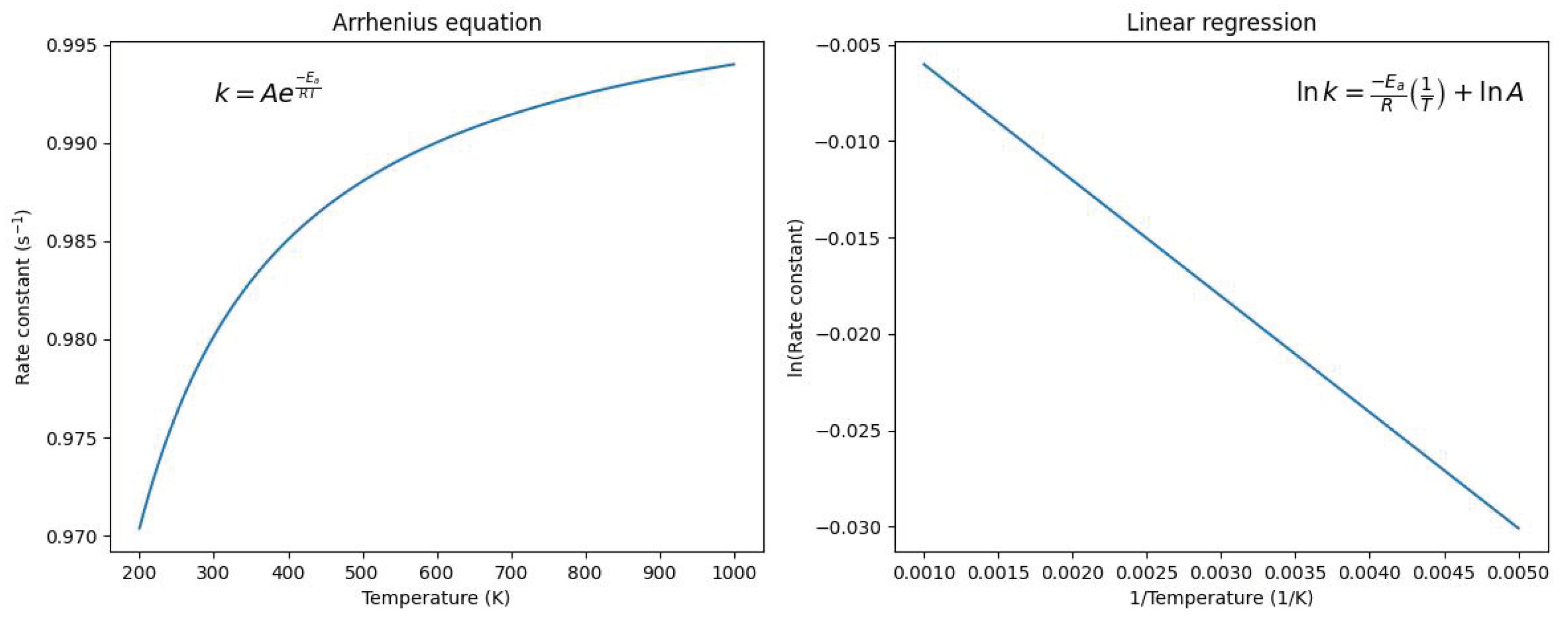
The need for the Arrhenius Equation arises from a lack of a mathematical expression linking the multiple factors that influence the rates of chemical reactions (Figure 1). At the time, the dominant viewpoint asserts that chemical reactions occur as a result of collisions between molecules possessing sufficient kinetic energy to bypass the energy barrier. Arrhenius then built on this idea and proposed a model that relates both the activation energy along with a physical justification and interpretation of the formula.

However, the Arrhenius Equation is best seen as an empirical relationship, because although it models reaction mechanisms, it does not provide a solid theoretical explanation as to why the rate constant changes with temperature, but rather describes the mathematical relationship between them. Furthermore, the reaction is not valid for every kind of reaction. For example, it does not describe accurately enzymatic reactions, microbiological growth, or other reactions having an optimal temperature.

Nevertheless, it is important to understand the mathematical context behind the Arrhenius equation because it is a cornerstone of chemical kinetics that has a wide range of applications, industrial chemistry, atmospheric chemistry and the study of reactions under extreme conditions. By providing a detailed analysis of the Arrhenius equation and its drawbacks, this paper contribute to a deeper understanding of chemical kinetics and inform future research in this field.

2. Exponential Term

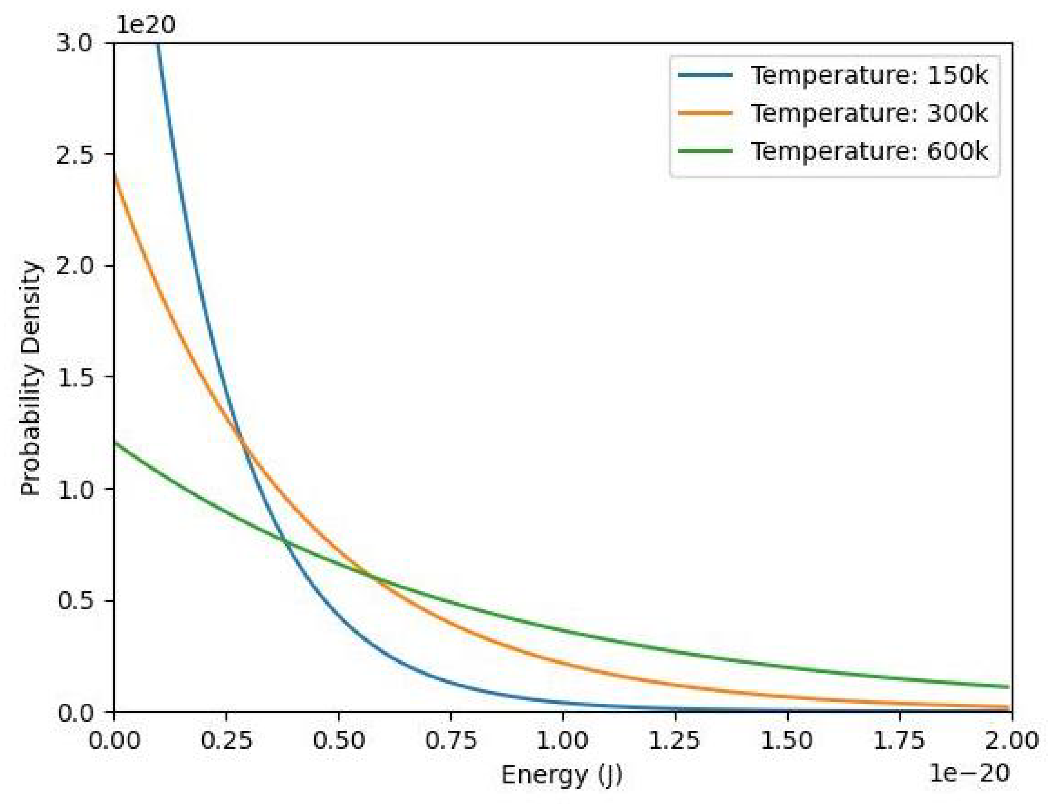
The exponential term in the Arrhenius Equation is arguably the most crucial component which effectively allows the equation to model chemical kinetics with great accuracy. It accounts for the proportion of reactant molecules which possess sufficient kinetic energy to cross the energy barrier and attain the state of activated complex. It considers both the activation energy of a specific reaction and the distribution of particle velocities. Hence, the exponential term is written as a function of temperature and activation energy.

Figure 2. Denormalized Boltzmann distribution of particle energy probability density at different temperatures.

The most direct derivation of the exponential term borrows the theories of statistical mechanics – most notably the Boltzmann distribution, P, which describes the probability of finding a particle at a certain energy level. The Boltzmann function is a normal distribution function expressed by the following function[1]:

P = C e^{\frac{- ϵ_{i}}{k_{B} T}}

(1)

where C is the normalization constant,

ϵ_{i}

is an arbitrary energy level and

k_{B}

is the Boltzmann constant (

k_{B} = 1.380649 \times 10^{- 23} \frac{J}{K}

). To calculate the probability of finding a particle whose kinetic energy is comprised within the interval

ϵ_{i}

ϵ_{i} + d ϵ_{i}

, we can simply multiply the distribution by the differential of energy:

P d ϵ_{i}

. This can later be integrated over the domain of interest.

However, the rate of chemical reactions if often measured in moles of reactants instead of individual particles. Therefore, we must express the Boltzmann distribution of particle velocity in terms of the sum of all energy in a mole of particles,

E_{i}

. We have that:

\begin{matrix} E_{i} = N_{A} \cdot ϵ_{i} \end{matrix}

(2)

\begin{matrix} d E_{i} = N_{A} d ϵ_{i} \end{matrix}

(3)

Rewriting the Boltzmann distribution in terms of

E_{i}

and simplifying using the relation

k_{B} N_{A} = R

P = C e^{\frac{- ϵ_{i}}{k_{B} T}} = C e^{\frac{- ϵ_{i} \cdot N_{A}}{k_{B} T \cdot N_{A}}} = C e^{\frac{- E_{i}}{R T}}

(4)

Now, before integrating the probability density function, it is necessary to normalize the distribution in terms of the constants R and

N_{A}

in such a way that the sum of all probabilities equals to 1. The normalization condition is given by

\int_{0}^{\infty} P d ϵ_{i} = 1

\begin{matrix} 1 & = \int_{0}^{\infty} \frac{P}{N_{A}} d E_{i} \\ = \int_{0}^{\infty} \frac{C}{N_{A}} e^{\frac{- E_{i}}{R T}} d E_{i} \\ = {[\frac{C}{N_{A}} (- R T) e^{\frac{- E_{i}}{R T}}]}_{0}^{\infty} \\ = \frac{R T C}{N_{A}} \\ C & = \frac{N_{A}}{R T} \end{matrix}

Plugging the normalization constant C into equation 4 and multiplying by the differential of energy yields the desired probability density function:

P d ϵ_{i} = \frac{N_{A}}{R T} \cdot e^{\frac{- E_{i}}{R T}} \cdot \frac{d E_{i}}{N_{A}} = \frac{e^{\frac{- E_{i}}{R T}}}{R T} d E_{i}

(5)

This allows us to compute the probability to find one particle whose kinetic energy is higher than the activation energy by integrating from

E_{A}

to infinity.

\frac{1}{R T} \int_{E_{a}}^{\infty} e^{\frac{- E_{i}}{R T}} d E_{i} = \frac{- R T}{R T} {[e^{\frac{- E_{i}}{R T}}]}_{E_{a}}^{\infty} = e^{\frac{- E_{a}}{R T}}

3. Modelling the Pre-exponential Factor

The pre-exponential factor (A) in the Arrhenius equation – also called the frequency factor – is an important variable which accounts for both the frequency of collisions between reactant molecules and the probability that the molecules collide in the right geometry to produce an activated complex. The pre-exponential factor can be evaluated both experimentally and through mathematical calculations.

In this section, we will attempt to build a mathematical model to approximate the pre-exponential factor of a bimolecular gaseous reaction in accordance with the principles of collision theories. This can be done by calculating the theoretical reaction rate using collision frequency and then comparing the value with the reaction rate predicted by the rate law and the Arrhenius equation.

3.1. Collision Frequency

We will start by calculating the collision frequency within the reaction vessel. To achieve this, we will assume that all particles behave like hard spheres with a defined radius. The reaction may only occur when the particles undergo a full collision.

Suppose that we have a container filled with gas particles A. We can determine the collision frequency for a single molecule,

Z_{A}

, by freezing all other atoms within the container and count the number of collisions within a period of time. [2] The number of collisions can be calculated using the following formula.

Z_{A} = \frac{Volume of Collisional Cylinder \times Density}{Time}

(7)

This equation can be later generalized to find the collision frequency for two different types of molecules,

Z_{A B}

3.1.1. Volume of Collision Cylinder

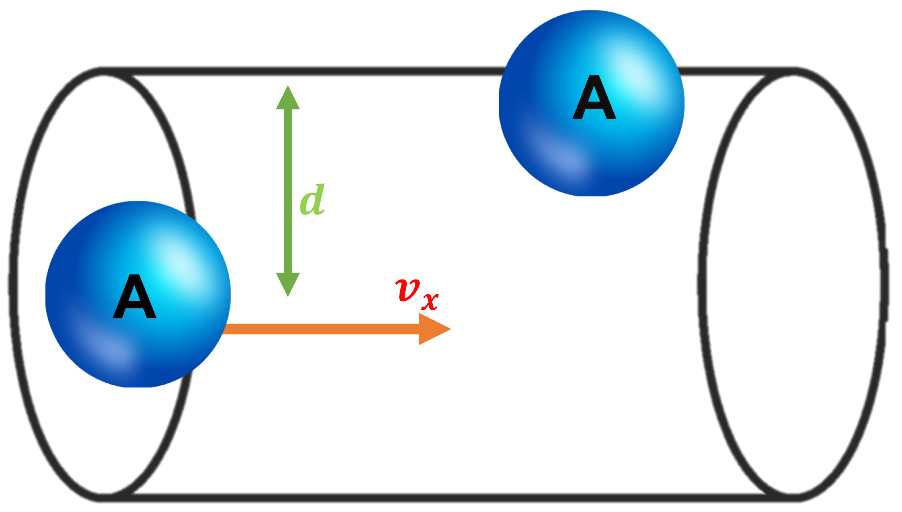
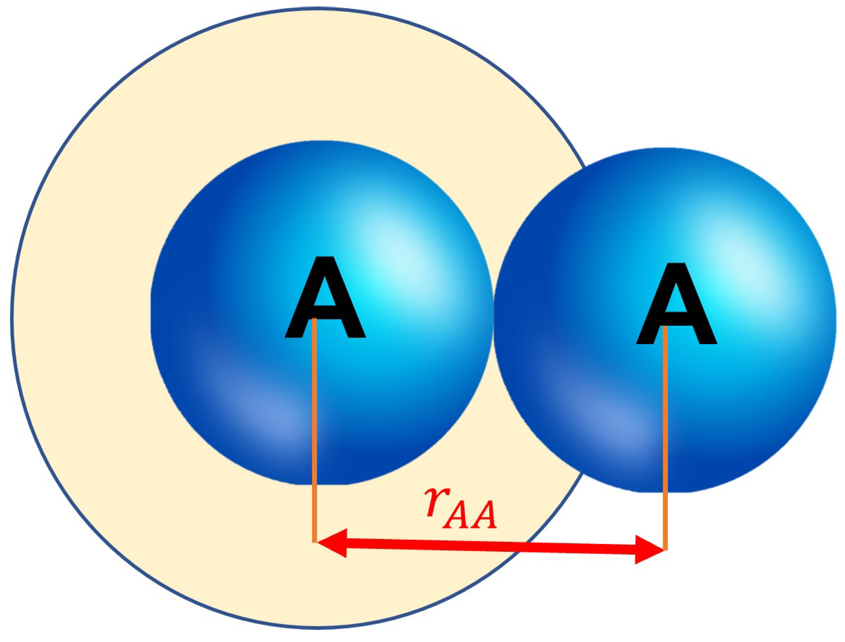
The Collision Cylinder (Figure 3) can be viewed as the volume whose cross-sectional area – the Collision Cross Section – contains the center of the second particle if the two particles are aligned to collide in the future. This can be better visualized in the Figure 4. Simply put, it is a volume swept out by the particle A in a time period

Δ t

[?].

Note that although a collision will like likely change the direction of the moving particle, this does not affect the volume of the Collision Cylinder nor the density within the system. Thus, the equation will hold true from one collision to the next.

We can find the area of the collision cross section with the area formula of a circle:

σ_{A A} = π r_{A A}^{2} = π {(2 r_{A})}^{2}

(8)

The sum of the radius of two identical spheres can also be expressed as their diameter,

d_{A}

σ_{A A} = π r_{A A}^{2} = π {(d_{A})}^{2}

(9)

Using equation 3, the volume of the collision cylinder is given by:

\begin{matrix} V & = σ_{A A} \cdot c_{A} \cdot Δ t \\ = π {(d_{A})}^{2} \cdot c_{A} \cdot Δ t \end{matrix}

(10)

where

c_{A}

is the mean speed of particle A and

Δ t

is an arbitrary amount of time.

3.1.2. Collision Frequency for a Single Particle A

Knowing the volume of the collision cylinder, the next parameter that needs to be taken into account is the number density of the molecules within the system, that is the number of a specific type of molecule within a unit volume. This will let us know the expected number of collisions within a time frame. The number density can be simply computed as:

ρ = \frac{N_{A}}{V}

(11)

where

N_{A}

is the number of particles A within the system and V is the volume of our container.

Plugging the equations 4 and 5 into the equation 1 yields the collision frequency of a single particle A.

\begin{matrix} Z_{A} & = \frac{π {(d_{A})}^{2} \cdot c_{A} \cdot Δ t \cdot \frac{N_{A}}{V}}{Δ t} \\ = \frac{π {(d_{A})}^{2} \cdot c_{A} \cdot N_{A}}{V} \end{matrix}

(12)

3.1.3. Collision Frequency for all Particles A

Now, every particle in the container starts moving again. It is possible to compute the collision frequency of all the A molecules,

Z_{A A}

, through the following relation:

Z_{A A} = \frac{1}{2} \cdot Z_{A} \cdot \frac{N_{A}}{V}

(13)

This relation accounts for the fact that every A molecule in the system can collide with another molecule in the same mechanism described above, thus we multiply it with the number density of A. Further, every collision is counted twice, thus we half the number.

Plugging the equation 6 into 7 yields:

\begin{matrix} Z_{A A} = \frac{π {(d_{A})}^{2} \cdot c_{A}}{2} \cdot {(\frac{N_{A}}{V})}^{2} \end{matrix}

(14)

3.1.4. Collision System Between Different Types of Molecules

The ultimate goal of the pre-exponential factor model is to build a general equation accounting for the collision frequency between two types of reactants,

Z_{A B}

. Namely, the equation should describe an elementary reaction of the type:

A_{(g)} + B_{(g)} \to product

The equation 8 can easily be modified to account for the change. We need only to modify the following elements:

1.: The collisional cross section should take into account the radius of both particles. Thus $d_{A}$ should be replaced with $r_{A} + r_{B}$ .
2.: The number of particles A and particles B could differ significantly within the container. To find the probability of a collision between these two types of particles, the particle density within the collisional cylinder should be replaced with the number density of the second particle, $\frac{N_{B}}{V}$ .
3.: There is no need to divide the collision frequency by two (look at equation 7) since we are now only counting the frequency of an A molecule striking B and not vice versa.
4.: Since we are considering a two bodied system, the mean speed of particle A should be replaced by the relative speed of particles A and B, $c_{A B}$ .

Rewriting equation 8 with the above modifications gives the following result:

Z_{A B} = π {(r_{A} + r_{B})}^{2} \cdot c_{A B} \cdot \frac{N_{A} N_{B}}{V^{2}}

(15)

Furthermore,

c_{A B}

could be expanded using the formula of mean gas particle velocity.

c = \sqrt{\frac{8 k_{B} T}{π m}}

(16)

However, since we are converting a two bodied system to a one-body system, it is important to use the reduced mass of particles A and B. The reduced mass is found by[2]:

μ_{A B} = \frac{m_{A} m_{B}}{m_{A} + m_{B}}

Plugging equation 10 into 9 yields the desired result for collision frequency:

Z_{A B} = \frac{N_{A} N_{B}}{V^{2}} {(r_{A} + r_{B})}^{2} \sqrt{\frac{8 π k_{B} T}{μ_{A B}}}

(17)

Finally, we can find the collision frequency as a function of the concentration of both reactants,

A_{A B}

, rather than as individual molecules. Thus, we divide both sides of the equation by

N_{a v o}^{2}

where

N_{a v o}

is the Avogadro’s number and substitute

\frac{n_{A}}{V}

C_{A}

and

\frac{n_{B}}{V}

C_{B}

A_{A B} = N_{a v o} C_{A} C_{B} {(r_{A} + r_{B})}^{2} \sqrt{\frac{8 π k_{B} T}{μ_{A B}}}

(18)

3.2. Pre-Exponential Factor

Now that we have developed a formula for the collision frequency for bimolecular gases reactions, we can use the equation to find the pre-exponential factor by comparing with the reaction rate predicted by classical rate law and the Arrhenius equation. In other words, we isolate the pre-exponential term equivalent in the collision frequency formula.

3.2.1. Reaction Rate According to the Collision Theories

According to collision theories, the rate of a chemical reaction will directly be affected by the following 3 factors:

1.: The ratio of particles possessing a sufficient amount of kinetic energy. When colliding, this energy is transformed to potential energy in order to bypass the activation energy barrier, $E_{a}$ .
2.: The number of collisions within a unit time period.
3.: The particles collide in the exact geometry in such a way that their electrons cloud interact with one another. This coefficient is called the orientation factor. 1

The ratio of molecules with sufficient kinetic energy is equal to the exponential term while the number of collisions is given by the equation 12 as the collision frequency. Taking these factors into consideration, the rate of a bimolecular reaction,

\frac{- d C_{A}}{d t}

is expressed as:

\frac{- d C_{A}}{d t} = N_{a v o} C_{A} C_{B} {(r_{A} + r_{B})}^{2} \sqrt{\frac{8 π k_{B} T}{μ_{A B}}} \cdot e^{\frac{- E_{a}}{R T}}

(19)

Note that we can also obtain the reaction rate using classical the rate law for elementary reactions:

\frac{- d C_{A}}{d t} = k C_{A} C_{B}

(20)

Substituting the rate constant k with the Arrhenius equation, we get:

\frac{- d C_{A}}{d t} = A e^{\frac{- E_{a}}{R T}} \cdot C_{A} C_{B}

(21)

Equating equations 13 and 15 and cancelling identical terms yields the desired result of our model:

\begin{matrix} A e^{\frac{- E_{a}}{R T}} \cdot C_{A} C_{B} & = N_{a v o} C_{A} C_{B} {(r_{A} + r_{B})}^{2} \sqrt{\frac{8 π k_{B} T}{μ_{A B}}} \cdot e^{\frac{- E_{a}}{R T}} \\ A & = N_{a v o} {(r_{A} + r_{B})}^{2} \sqrt{\frac{8 π k_{B} T}{μ_{A B}}} \end{matrix}

3.3. Limitations of the Model

Although the mathematical model of the pre-exponential factor offers a general approximation, it often does not give an exact value. In fact, in some cases (as listed below), the errors add up to one another, making the gap between our approximate and the empirical value quite significant. Even small variations in the particles’ characteristics - including their mass and radius - may have an enormous influence on the final value of the pre-exponential factor. All these errors mainly arise from the limits of the collision theories, which do not provide a detailed account of the mechanism during a reaction. The following is a list of assumptions we made to simplify the problem [?]:

1.: It is assumed that all particles behave like hard spheres with a defined radius and a defined position. However, in reality, atoms react when their electron clouds come sufficiently close together to interact with one another. The electron cloud is consisted of a probability range, which means there is not a precisely defined distance below which atoms react.
2.: It is assumed that every collision in which the particles possess sufficient kinetic energy will undergo chemical transformation. This statement does not reflect the reality, as molecules must imperatively hit one another in the precise geometry to form an activated complex.
3.: In the collision theory, only the kinetic energy of particles is considered, while rotation and vibration energies are ignored.

Furthermore, this model has a restrained scope of usage, as it can only be applied to bimolecular reactions with all reactants in a gaseous state. Particles behave slightly differently in aqueous solutions, as they will have a different average velocity. The transition state theories generally offer a quantitative understanding of chemical reactions in solutions.

4. Conclusion

The Arrhenius equation proved to be an essential tool in understanding various molecular aspects of chemical reactions including activation energy requirements and temperature dependence. Further modelling of the pre-exponential factor using collision theory unveils its dependence on temperature, atomic radius and gas speed. It is important to note, however, that the collision theory does not offer a precise account of the reaction mechanism because several assumptions were made to simplify the problem. Advanced modelling will be necessary to understand chemical reactions in deeper detail. Nevertheless, the results shown in this paper can be combined with other formulas and are essential for both basic reaction analysis and for advanced kinetic modelling. These advances along with improving computational methods have made possible the optimization of existing chemical reactions and the development of new industrial processes.

References

McQuarrie, D.; Simon, J. Physical Chemistry: A Molecular Approach, Chapter 4; Physical Chemistry: A Molecular Approach, University Science Books, 1997.
Laidler, K.J. Chemical Kinetics, chapter 4; Chemical Kinetics, Person, 1987.

1	The orientation factor will not be discussed in this demonstration as it is highly dependent on the type of reactant and cannot be generalized in by a simple formula.

Figure 1. Arrhenius equation of reaction constant, k, as a function of temperature, T on the left and its linear regression on the right.

E_{a} = 50 \frac{k J}{m o l}

Figure 1. Arrhenius equation of reaction constant, k, as a function of temperature, T on the left and its linear regression on the right.

E_{a} = 50 \frac{k J}{m o l}

Figure 3. Collision Cylinder of Atom A

Figure 4. Collision Cross Section of atom A and B

Disclaimer/Publisher’s Note: The statements, opinions and data contained in all publications are solely those of the individual author(s) and contributor(s) and not of MDPI and/or the editor(s). MDPI and/or the editor(s) disclaim responsibility for any injury to people or property resulting from any ideas, methods, instructions or products referred to in the content.

© 2023 by the authors. Licensee MDPI, Basel, Switzerland. This article is an open access article distributed under the terms and conditions of the Creative Commons Attribution (CC BY) license (http://creativecommons.org/licenses/by/4.0/).

Copyright: This open access article is published under a Creative Commons CC BY 4.0 license, which permit the free download, distribution, and reuse, provided that the author and preprint are cited in any reuse.

MDPI Initiatives

Important Links

Choose an area of interest and we will send you notifications of new preprints at your preferred frequency.

Disclaimer

Deriving the Arrhenius Equation and the Pre-Exponential Factor

Abstract

1. Introduction

2. Exponential Term

3. Modelling the Pre-exponential Factor

3.1. Collision Frequency

3.1.1. Volume of Collision Cylinder

3.1.2. Collision Frequency for a Single Particle A

3.1.3. Collision Frequency for all Particles A

3.1.4. Collision System Between Different Types of Molecules

3.2. Pre-Exponential Factor

3.2.1. Reaction Rate According to the Collision Theories

3.3. Limitations of the Model

4. Conclusion

References

MDPI Initiatives

Important Links

Subscribe