
You are currently viewing a beta version of our website. If you spot anything unusual, kindly let us know.
Preprint
Article
Research on SLAM and Path Planning Method of Inspection Robot in Complex Scenarios
Altmetrics
Downloads
138
Views
24
Comments
0
A peer-reviewed article of this preprint also exists.

This version is not peer-reviewed
Abstract
Factory safety inspections are crucial for ensuring safe production. However, manual inspections present issues such as low efficiency and high workload. Inspection robots provide an efficient and reliable solution for completing patrol tasks. The development of robot localization and path planning technologies provides guarantees for factory inspection robots to autonomously complete inspection tasks in complex environments. This paper studies mapping and localization, as well as path planning methods for robots in order to meet the application requirements of factory inspections. Two SLAM application systems based on multiple-line laser radar and vision are designed for different scenarios in consideration of the limitations of cameras and laser sensors in terms of their own characteristics and applicability in different environments. To address the issue of low efficiency in inspection tasks, a hybrid path planning algorithm that integrates the A-star algorithm and time elasticity band algorithm is proposed. This algorithm effectively solves the problem of path planning in complex environments that is prone to falling into local optimal solutions, thereby improving the inspection efficiency of robots. Experimental tests show that the designed SLAM and path planning methods can meet the needs of robot inspection in complex scenes and have good reliability and stability. The code used in this article is open source and can be accessed at https://github.com/Mxiii99/RSPP_CS.git.
Keywords:
Subject: Computer Science and Mathematics - Robotics
1. Introduction
With the introduction of "Industry 4.0", robotics technology has rapidly advanced. Among them, inspection robots have been extensively used in aerospace, manufacturing, agriculture, service industries, and other fields due to their superior flexibility, mobility, and functionality [1,2]. As inspection application scenarios become more diversified and complex, higher requirements are placed on the autonomous navigation performance of robots. Robot navigation technology mainly consists of SLAM technology and path planning technology. Simultaneous Localization and Mapping (SLAM) is the process by which a mobile robot determines its own position and creates a map through sensors carried in the surrounding environment. Path planning technology creates the optimal navigation path for the robot to reach the target location based on different task goals and requirements.
SLAM technology can be classified into two categories based on different sensors: vision-based and LIDAR-based. The MonoSLAM method proposed by Davison et al. estimates the camera pose by extracting sparse feature points frame by frame, which is the first real-time visual SLAM system using a single camera [3]. Subsequently, Klein et al. proposed the PTAM method, which introduced nonlinear optimization and keyframe mechanism [4], solving the problem of high computational complexity in MonoSLAM. Newcombe et al. proposed a dense per-pixel method based on RGB-D camera, which can achieve real-time tracking and reconstruction [5]. As for LIDAR-based SLAM methods, Grisetti et al. proposed a 2D SLAM algorithm based on particle filtering, which solved the problem of particle dissipation caused by resampling through reducing the number of particles [6]. Konolige et al. proposed the first open-source algorithm based on graph optimization by using highly optimized and non-iterative square-root factorization to sparsify and decouple the system [7]. Kohlbrecher et al. designed the Hector SLAM algorithm, which matches the current frame’s LIDAR data with the factor graph and optimizes the pose using the Gauss-Newton method to obtain the optimal solution and bias [8].
Path planning is to plan a collision-free optimal path from the starting point to the destination point in the map environment. Path planning can be divided into global and local path planning according to whether the environment information is known in advance. Dijkstra et al. proposed the shortest path planning algorithm, which uses breadth-first search to search for paths [9]. Hart et al. proposed the A-star algorithm, which reduces the search nodes by using heuristic evaluation function and improves the efficiency of path searching [10]. Fox et al. proposed the DWA, which samples velocity dynamically in the robot’s sampling space according to the robot’s kinematic model and current motion parameters, and selects the best trajectory [11]. To address the insufficient evaluation function of DWA, Chang et al. proposed an improved DWA algorithm based on Q-learning, which modifies and extends the evaluation function and adds two evaluation functions to improve navigation performance and achieve higher navigation efficiency and success rate in complex unknown environments [12]. Rösmann et al. proposed the Time Elastic Band algorithm based on multi-objective optimization, which ensures that the robot can output a smooth trajectory under the premise of satisfying its kinematic constraints [13].
Both lidar and camera sensors are essential for factory inspections, but their applicability depends on the specific application scenarios and factory environments. Lidar is suitable for long-distance and high-precision measurements, such as inventory management in large warehouses and position control in robot operations. However, lidar has limitations in processing details and colors, making it unsuitable for high-visual requirements scenes. Camera sensors, with their functions such as image recognition, detection, and tracking, are ideal for environments that require high-precision visual detection and recognition, such as detecting product dimensions, shapes, colors, and performing automated visual inspections during assembly processes on production lines. In addition, camera sensors have strong processing capabilities for details and colors, providing more detailed image information. However, camera sensors are highly dependent on ambient light, which can limit their effectiveness in poor lighting conditions or when obstacles are present.
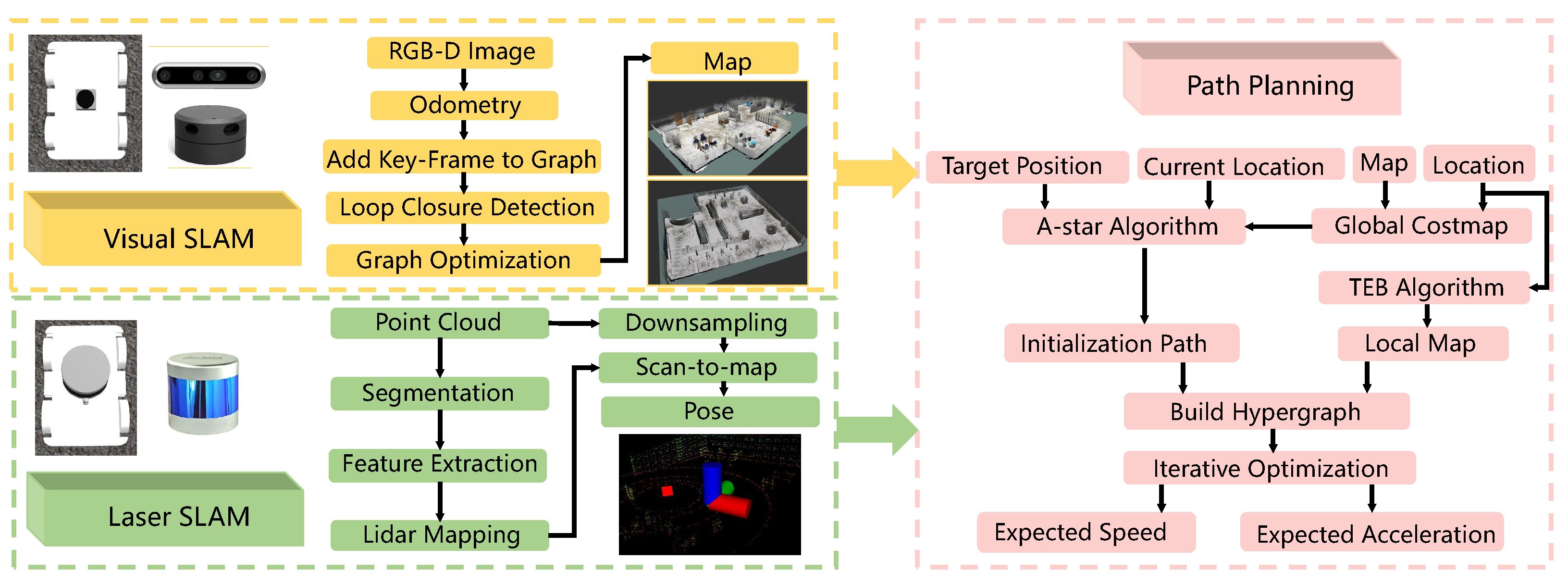
In this article, we designed two sets of SLAM systems based on multi-line lidar and vision sensors respectively to meet the inspection needs of robots in different environments. Global path planning using the A-star algorithm was adopted to improve navigation efficiency and help robots quickly plan the optimal path, reducing inspection time and costs. However, the A-star algorithm is not suitable for dynamic environments. Therefore, we introduced the Time Elastic Band algorithm, a real-time path planning algorithm that can adapt to changes in the environment and obstacles, resulting in more optimized path planning results to improve the efficiency of robot inspections and reduce collisions and other safety issues between robots and factory equipment. The method proposed in this article adopts a global and local fusion path planning algorithm for both lidar SLAM and vision SLAM, ultimately achieving autonomous navigation and obstacle avoidance of inspection robots in comple.
Figure 1.
System framework.
2. Inspection robot SLAM system
2.1. Visual-SLAM Algorithm Design and Implementation
In the factory environment, the position and motion of inspection robots and equipment may undergo rapid changes, thus requiring real-time acquisition and processing of sensor data for accurate localization and mapping. To achieve this, we have chosen an appearance-based localization and mapping method that is invariant to time and scale, as shown in the structural diagram in Figure 2.
From Figure 2, it can be seen that RGB-D images are used as external input, and the ORB algorithm is used to extract feature points from RGB-D images [14]. Then, a Bag-of-Words based image matching method is used to match feature points between adjacent frames. The loop-closure detection mechanism is introduced to eliminate drift. When the robot returns to an area previously visited, the loop-closure detection can identify the area and match the newly observed data with the previous map data, thus addressing the cumulative drift problem. Next, graph optimization is performed, where the robot’s poses are represented as nodes in the graph and the observed data is represented as edges. Then, the least squares method is used to optimize the positions of all nodes, minimizing the error between observed and predicted data. Finally, a dense map can be generated.
This vision-based mapping and localization algorithm utilizes global and local loop-closure detection techniques, which can identify and handle errors and drift in sensor data, improving the robustness and accuracy of localization and mapping, and enhancing the efficiency and real-time performance of inspection robots.
2.2. Multi-line LiDAR-based SLAM Algorithm Design and Implementation
In indoor factory environments, lighting conditions can vary with time and location, which may lead to misidentification of objects or inaccurate positioning by visual sensors. However, laser sensors do not require an external light source, as they emit their own laser beams and are not affected by lighting issues. Therefore, we have adopted a lightweight and ground optimized laser odometry and mapping method, whose structural diagram is shown in Figure 3. Firstly, the laser point cloud data is dimensionally reduced, projecting the 3D laser onto a 2D depth image, segmenting the ground according to the pitch angle, clustering non-ground point clouds, and obtaining labeled point cloud data. Then, feature extraction is performed based on smoothness, resulting in four sets of feature point clouds. Constraint relationships are established for the feature point cloud sets, and the 6-DOF pose transformation matrix is solved using the Levenberg-Marquardt (LM) optimization method. Subsequently, loop detection is conducted using the Iterative Closest Point (ICP) algorithm, and finally, the current point cloud is mapped to the global map based on graph optimization, completing the establishment of a high-precision map [15].
1) Point cloud segmentation: Due to the complexity of the inspection environment and other factors, noise may exist in the laser point cloud data. We first use point cloud segmentation to filter out noise. By projecting a frame of 3D point cloud onto a 2D depth image using a projection method, ground segmentation is performed to separate non-ground points [16]. Let be the point cloud data obtained by the lidar at time t, where is a point in . These points are projected onto a depth image, and the 3D points in space become 2D pixels in space. After projection, the Euclidean distance of point to the sensor is obtained. Since the 3D point cloud contains a large amount of ground information, it is necessary to filter the point cloud to improve the efficiency and accuracy of feature extraction. Firstly, the ground points are labeled, and the labeled ground points will no longer be segmented in subsequent steps. After separating ground points and non-ground points, the non-ground points are processed by clustering. After this module, each point has its own segmentation label (ground or non-ground), row and column indices in the depth image, and the Euclidean distance to the sensor.
2)Feature extraction: According to the smoothness, the projected depth image is horizontally divided into several sub-images. For each sub-image, the following process is performed [17]: Let S be the set of continuous points in the same row in the depth image, and calculate the smoothness c of point .
where and are the Euclidean distances from points and to the sensor. According to Equation (1), the smoothness of each point can be calculated, and then the smoothness is sorted. After sorting, feature points are selected. Different types of features are segmented based on the set threshold . The edge points with a smoothness c greater than are selected as set , and the plane points with a smoothness c less than are selected as set . The largest edge points with the maximum c value and the smallest plane points with the minimum c value are selected from all sub-images to form the edge feature point set and the plane feature point set . Then, edge points not belonging to ground points with the maximum c value are selected from set to form set , and plane points belonging to ground points with the minimum c value are selected from set to form set . Obviously .
3)Radar Odometry: The odometry module estimates the robot’s pose change between adjacent frames using a radar sensor. In the estimation process, tag matching is used to narrow down the matching range and improve accuracy, and a two-step LM optimization method is used to find the transformation relationship between two consecutive frames [18]. The first step uses ground feature points to obtain , and the second step matches the edge features extracted from the segmented point cloud to obtain the transformation . Finally, by fusing and , a 6-DOF pose transformation matrix is obtained.
4)Radar Mapping: After obtaining the pose change between adjacent frames with radar odometry, the features in the feature set at time t are matched with the surrounding point cloud to further refine the pose transformation. Then, using the LM optimization, the final transformed pose is obtained and the pose graph is sent to GTSAM for map optimization to update the sensor estimated pose and the current map [19].
In addition, noise may exist in the collected laser point cloud data. In order to achieve high-precision localization on the map, it is necessary to preprocess the high-precision map. We use a statistical-based robust filter to remove outliers, a pass-through filter to clip the point cloud within a specified coordinate range, and a voxel grid filter to downsample the point cloud. For the inspection task that requires high-precision real-time localization, we perform real-time localization on the constructed high-precision map through point cloud registration. First, the reference point cloud (i.e., high-precision map) is transformed into a multivariate normal distribution [20]. If the transformation parameters can accurately match the reference point cloud and the current point cloud, the transformed points in the reference frame have a high probability density. Therefore, an optimization method can be used to calculate the transformation parameters that maximize the sum of the probability densities. In this case, the two sets of laser point cloud data match best. The specific algorithm steps are as follows:
1) Given the current scanning point cloud S and the reference point cloud T, the space occupied by the T point cloud is divided into voxel grids of a specified size, and the expected vector and covariance matrix of N points in each voxel grid are calculated.
Here, represents the three-dimensional coordinates of the point cloud in the voxel grid.
2) Initialize the transformation parameters to be solved, with zero values or odometry data. For each sample in the S point cloud, transform it to the T point cloud according to the transformation parameters. Let be the coordinate of in the T point cloud coordinate system. Find the grid where falls in the T point cloud, and combine the probability density function of each grid in the T point cloud to calculate the corresponding probability distribution function .
3) Add up the probability densities calculated for each mapped point to obtain the registration score.
Use the Newton optimization algorithm to optimize the objective function until the optimal transformation parameters are found that maximize the registration score, complete convergence, and solve the best rigid body transformation between the target and source point clouds to achieve accurate localization.
3. Inspection robot Path planning system
3.1. Sports model
Currently, the chassis of inspection robots mainly consists of legged, tracked, and wheeled types, each with its advantages and disadvantages in different environments. Legged inspection robots have strong terrain adaptability, but their structure and control system are complex. Tracked inspection robots have high traction and strong applicability in complex terrains such as outdoor, sandy, and muddy areas, but their speed is relatively low, and they have high motion noise. Wheeled inspection robots have fast speed, high efficiency, and low motion noise, and are widely used. In this paper, we focus on the complex indoor factory environment and adopt a two-wheel differential wheeled robot whose kinematic model is shown in Figure 4 [21].
In Figure 4, the motion of robot is completed by two independently driven wheels. Let the radius of the driving wheel be , and define the midpoint of the two driving wheels as . The distance between the two wheels is , where is the inertial Cartesian coordinate system, and is the local coordinate system of the robot. is the speed of the left driving wheel, is the speed of the right wheel, and is the speed of the center of the robot. If , the angular velocity can be obtained. According to the robot model, the forward speed depends on the speed of the wheels.
The angular velocity is determined by the difference in speed between the left and right driving wheels and the distance between them.
In the ideal case, according to the principle of rigid motion, the trajectory of the robot is a circle, and the radius can be expressed as
The kinematic equation of the robot can be expressed as
The above formula is the pose state matrix and motion state matrix, and the final formula can be written as follows:
where is a smooth linearly independent matrix, and V is the motion matrix of the robot.
3.2. Path Planning
The path planning of inspection robots mainly relies on the constructed grid map to generate a safe and collision-free path by specifying the start and target locations. The path planning for robots can be divided into global path planning and local path planning.
(1) Global path planning
To ensure that the patrol robot can effectively avoid obstacles globally and locally, and considering that the grid map of the actual road scene is relatively simple, the A-star algorithm is used as the global path planning method to provide accurate obstacle avoidance directions for the robot through real-time planning [22,23]. A-star combines heuristic search with breadth-first algorithm to select the search direction through the cost function , and expands around the starting point. The cost value of each surrounding node is calculated by the heuristic function , and the minimum cost value is selected as the next expanding point. This process is repeated until the endpoint is reached, generating a path from the starting point to the endpoint. In the search process, since each node on the path is the node with the minimum cost, the cost of the path obtained is also minimum. The cost function of the A-star algorithm is
where is the cost function at the current position, is the cost value from the starting position to the current position in the search space, and is the cost value from the current position to the goal position. In the A-star algorithm, the selection of the heuristic function is crucial. Since the map environment is a grid map with obstacles, the Manhattan distance is used as the heuristic function, which is given by:
where , represent the coordinates from the current position to the target position. In the path planning of the A-star algorithm, the nodes are stored in two lists, Closelist and Openlist. The nodes that have been searched and generated cost values are stored in Openlist. The node with the minimum estimated cost is stored in Closelist, and the moving trajectory is formed by processing the trajectories of each node in Closelist. The specific steps are as follows:
Step 1.The starting point s of the robot is the first calculated point, and the surrounding nodes are added to Openlist, and the cost function of each point is calculated.
Step 2.Search Openlist, select the node with the smallest cost value as the current processing node n, remove the node from Openlist, and put it into Closelist.
Step 3.If the real cost value of the adjacent node from the current processing node to the starting point s is smaller than the original value, the parent node of the adjacent node is set to the current processing node; if it is larger, the current processing node is removed from Closelist, and the node with the second smallest value of is selected as the current processing node.
Step 4.Repeat the above steps until the target point g is added to Closelist, traverse along each parent node, and the obtained node coordinates are the path.
(2)Local path planning
The working environment of inspection robots is not always static. In the process of moving along the global path, real-time obstacles may appear. To avoid collisions, the Timed-Elastic-Band (TEB) algorithm, which introduces local path planning with time elasticity, is used on the basis of global path planning to achieve real-time obstacle avoidance [24]. The TEB algorithm is an optimization algorithm that follows the path generated by the global path planner. The local trajectory it generates is composed of a series of continuous time and pose sequences, and the robot’s pose is defined as:
where represents the i-th pose in the robot coordinate system, including position information , and angle . The time interval between adjacent poses and is denoted by , as shown in Figure 5.
In the optimization process, the TEB algorithm applies graph optimization to the adjacent time intervals and states of the robot as nodes, and uses velocity, acceleration, and non-holonomic constraints of the robot as edges. It also considers obstacle information, discrete interval of planned trajectory, and adjacent temporal and spatial sequence constraints. Finally, the G2O solver is used to calculate the control variable (where v and represent the linear and angular velocity of the robot, respectively), to obtain the optimal trajectory. The TEB algorithm obtains the optimal pose points through weighted multi-objective optimization [25,26], where the mathematical description of the objective function is:
where is the objective function that considers various constraints, is the constraint function, is the weight of each item, and is the optimal TEB trajectory. The TEB algorithm has four constraint functions.
1) Path following and obstacle constraint objective function
The TEB algorithm aims to avoid collisions with static or dynamic obstacles while following the path. The algorithm treats piecewise continuous and differentiable functions as constraints and punishes behaviors that do not conform to the constraints. Specifically:
Building on Equation (18), penalty functions and are constructed. Here, denotes the boundary, is the offset factor, S is the scaling factor, n is the order, is the independent variable representing the distance between the path point and obstacle, is the maximum distance of the trajectory deviation from the path point, and is the minimum distance between the trajectory and obstacle.
2) The velocity and acceleration constraint functions of a robot
According to the dynamic equation, the constraint functions of the robot’s velocity and acceleration are expressed as equations (21) - (24) :
Linear velocity:
Angular velocity:
Linear acceleration:
Angular acceleration:
3) Non-holonomic constraint:
The robot used in the algorithm simulation and experiment is a differential drive structure with two degrees of freedom, which cannot perform translational motion along the y-axis of the robot coordinate system. The curvature of the circular arc between two adjacent robot poses is approximately constant, and the outer product of the direction vector and the turning angle between adjacent poses in the robot coordinate system is equal to the outer product of the turning angle and the direction vector . represents the orientation of the robot in the global coordinate system, and the corresponding relationship equation and non-holonomic constraint are:
The objective function punishes the quadratic error for violating this constraint, ensuring that the output velocity of the robot follows the non-holonomic constraint.
4) Fastest path constraint
The TEB algorithm incorporates the time interval information between poses, and the total time is the sum of all time intervals. The relevant objective function is:
After optimizing the TEB sequence, the objective function of the constraints is optimized to ensure that the path planned by the algorithm achieves the best results in terms of obstacle avoidance, time, and distance.
(3)Path planning based on fusion algorithm
The A-star algorithm yields a navigation path consisting of only the start point, key points, and destination point, but it cannot avoid unknown obstacles in the environment. The TEB algorithm exhibits good local obstacle avoidance ability, but with only a single final goal point as a guide, it is prone to becoming trapped in local optima. Therefore, we propose a hybrid path planning algorithm that combines the strengths of both algorithms. The specific algorithm process is shown in Figure 6.
Global path planning takes a static obstacle cost map as input, and does not consider the robot’s mechanical performance and kinematic constraints when planning the path. It uses the A-star algorithm to plan the optimal path from the robot’s current position to the desired target position, and provides an initial value for local planning.
Local path planning collects path nodes on the global optimal path, and optimizes the global path subset between the robot’s current node and the collected path nodes. It combines the static obstacle cost map and dynamic obstacle cost map, and uses the TEB algorithm to continuously adjust the pose and orientation of the robot during its movement, taking into account its shape, dynamic model, and motion performance in the scope of local planning. When encountering dynamic obstacles, it removes the old robot pose and adds a new robot pose, so that a new path can be generated in each iteration, and an optimized path can be obtained through continuous iteration.
By fusing navigation algorithms, we achieve optimal global path planning and real-time obstacle avoidance functionality in the process of mobile robot navigation.
4. Experiment and Analysis
4.1. Experiment settings
In order to verify the effectiveness of navigation systems in practical applications, we conducted experiments using a Turtlebot3 mobile robot in different types of scenarios built using the Gazebo simulation platform within the ROS on a 64-bit Ubuntu 18.04 operating system with 4GB of running memory. As shown in Figure 7, we constructed a home environment and a library environment to simulate real-world environments. Using the real-time localization and mapping capabilities in Rviz, we scanned the simulated environments, constructed corresponding maps, and performed path planning.
4.2. Performance evaluation
4.2.1. Visual-SLAM Algorithm performance evaluation
This paper presents a method for constructing a corresponding point cloud map using a depth camera in a ROS environment. The depth camera data is first read in the ROS environment, and then the front-end and back-end threads are executed to construct a sparse feature point map, which is continuously updated to create a real-time point cloud map. Keyframes from the front-end are passed into the point cloud construction thread to generate the point cloud map. The effectiveness of the proposed algorithm for generating maps is validated by the corresponding point cloud map in Figure 8, which demonstrates good 3D effects for constructing maps in indoor environments. As shown in Figure 8, the algorithm detects the object’s motion trajectory, which is consistent with the actual trajectory. Although there are deviations between the detected trajectory and the actual trajectory, there is no serious deviation, which satisfies the perception requirements of the robot. When the object’s motion trajectory changes significantly, there is still no serious deviation, which also meets the perception requirements of the robot.
4.2.2. Multi-line LiDAR-based SLAM Algorithm performance evaluation
From the comparison between point cloud mapping and visual mapping, it can be observed that maps constructed using multi-line laser scanning are clearer than those constructed using visual algorithms, which reduces accumulated errors and provides better handling of edge contours. Furthermore, a comparison was conducted on mapping time, mapping effectiveness, and CPU utilization, in order to validate the feasibility, reliability, and accuracy of the algorithm.
To ensure the accuracy of the experiments, multiple tests were conducted. The robot was fixed at a certain position, denoted as the origin (0,0), and the output object motion data was compared with the actual object motion data. The results are shown in Figure 9. The algorithm detected that the point cloud map was generally consistent with the simulated scene, and that the detected trajectory was not significantly deviated from the actual trajectory, which satisfies the perception requirements of the robot. As shown in the figure, when there were large changes in the object’s motion trajectory, there was a slight deviation between the detected trajectory and the actual trajectory, but no serious deviation occurred, which still satisfied the perception requirements of the robot.
4.2.3. Path Planning Performance Evaluation
Through testing, the path distance planned by the A-star algorithm has a certain distance from the obstacles, which avoids the collision of the robot. At the same time, global path planning has a good effect and can accurately reach the set target point location, satisfying the requirement of precise navigation. The robot moves along a square path. When encountering obstacles, it autonomously avoids them through local path planning. The process and result of local path planning are shown in Figure 10. After configuring the relevant parameters, observe the 3D view area of robot navigation in Rviz. The environment of the map is displayed as a global cost map, and the environment around the robot is a local cost map. The blue area is the expansion layer of the obstacle, which is expanded outward on the map to avoid collision between the robot and the obstacle. By adding the Path plugin in RViz, you can see the path that the robot moves. The green line is the route of global path planning, and the red line is the route of local path planning. It can be seen from Figure 10 that the local path planning route of the inspection robot is smooth and the planned route does not enter the expansion layer of the obstacle, which can reasonably avoid the surrounding obstacles and has a good obstacle avoidance effect. The global path planning is shown in Figure 11. After testing, the inspection robot can accurately achieve autonomous obstacle avoidance and complete local path planning for the set target point, satisfying the requirement of precise navigation.
5. Conclusions
The utilization of intelligent inspection robots has been shown to enhance production efficiency and reduce costs. However, the complex factory environment, filled with machinery equipment, pipelines, cables, and other obstacles, can pose a challenge to accurate inspections. To address this, we have developed a high-precision navigation inspection system that is specifically designed for complex factory scenes. The system is equipped with two types of sensors, visual and LiDAR, to allow for rich environmental information and localization and mapping. Optimal path planning is achieved by combining the A-star algorithm and TEB algorithm for dynamic programming. To evaluate the performance of the navigation system, simulations were conducted in two scenarios using Gazebo simulation software in the ROS system: a residential area and a library. Results indicate that the navigation system provides real-time localization and map construction, can navigate mobile platforms, and implements real-time obstacle avoidance in different scenarios. As such, this technology can be applied to the localization and navigation system of wheeled inspection robots in various complex environments, and has significant reference value.
Author Contributions
Conceptualization, X.M. and X.W.; methodology, X.M. and X.W.; software, X.M. and X.W.; validation, X.M., X.W. and Z.L. All authors have read and agreed to the published version of the manuscript.
Funding
This research is funded by the Graduate Education and Teaching Quality Improvement Project of Beijing University of Architecture and Architecture (J2023017); the Lecturer Support Plan Project of Beijing University of Architecture and Architecture (YXZJ20220804); the Open Project of Anhui Provincial Key Laboratory of Intelligent Building and Building Energy Efficiency, Anhui Jianzhu University (IBES2020KF06); the BUCEA Post Graduate Innovation Project.
Informed Consent Statement
For studies not involving humans or animals.
Data Availability Statement
Not applicable.
Acknowledgments
Not applicable.
Conflicts of Interest
The authors declare no conflict of interest.
References
- Bahrin, M.A.K.; Othman, M.F.; Azli, N.H.N.; Talib, M.F. Industry 4.0: A review on industrial automation and robotic. Jurnal teknologi 2016, 78. [Google Scholar]
- Choi, H.; Ryew, S. Robotic system with active steering capability for internal inspection of urban gas pipelines. Mechatronics 2002, 12, 713–736. [Google Scholar] [CrossRef]
- Davison, A.J.; Reid, I.D.; Molton, N.D.; Stasse, O. MonoSLAM: Real-time single camera SLAM. IEEE transactions on pattern analysis and machine intelligence 2007, 29, 1052–1067. [Google Scholar] [CrossRef] [PubMed]
- Pire, T.; Fischer, T.; Castro, G.; De Cristóforis, P.; Civera, J.; Berlles, J.J. S-PTAM: Stereo parallel tracking and mapping. Robotics and Autonomous Systems 2017, 93, 27–42. [Google Scholar] [CrossRef]
- Zhou, H.; Ummenhofer, B.; Brox, T. DeepTAM: Deep tracking and mapping with convolutional neural networks. Springer, 2020, Vol. 128, pp. 756–769.
- Grisetti, G.; Kümmerle, R.; Stachniss, C.; Burgard, W. A tutorial on graph-based SLAM. IEEE Intelligent Transportation Systems Magazine 2010, 2, 31–43. [Google Scholar] [CrossRef]
- Strasdat, H.; Davison, A.J.; Montiel, J.M.; Konolige, K. Double window optimisation for constant time visual SLAM. 2011 international conference on computer vision. IEEE, 2011, pp. 2352–2359.
- Harik, E.H.C.; Korsaeth, A. Combining hector slam and artificial potential field for autonomous navigation inside a greenhouse. Robotics 2018, 7, 22. [Google Scholar] [CrossRef]
- Noto, M.; Sato, H. A method for the shortest path search by extended Dijkstra algorithm. Smc 2000 conference proceedings. 2000 ieee international conference on systems, man and cybernetics.’cybernetics evolving to systems, humans, organizations, and their complex interactions’(cat. no. 0. IEEE, 2000, Vol. 3, pp. 2316–2320.
- Seet, B.C.; Liu, G.; Lee, B.S.; Foh, C.H.; Wong, K.J.; Lee, K.K. A-STAR: A mobile ad hoc routing strategy for metropolis vehicular communications. Networking 2004: Networking Technologies, Services, and Protocols; Performance of Computer and Communication Networks; Mobile and Wireless Communications Third International IFIP-TC6 Networking Conference Athens, Greece, –14, 2004, Proceedings 3. Springer, 2004, pp. 989–999. 9 May.
- Ogren, P.; Leonard, N.E. A convergent dynamic window approach to obstacle avoidance. IEEE Transactions on Robotics 2005, 21, 188–195. [Google Scholar] [CrossRef]
- Chang, L.; Shan, L.; Jiang, C.; Dai, Y. Reinforcement based mobile robot path planning with improved dynamic window approach in unknown environment. Autonomous Robots 2021, 45, 51–76. [Google Scholar] [CrossRef]
- Rösmann, C.; Hoffmann, F.; Bertram, T. Timed-elastic-bands for time-optimal point-to-point nonlinear model predictive control. 2015 european control conference (ECC). IEEE, 2015, pp. 3352–3357.
- Ragot, N.; Khemmar, R.; Pokala, A.; Rossi, R.; Ertaud, J.Y. Benchmark of visual slam algorithms: Orb-slam2 vs rtab-map. 2019 Eighth International Conference on Emerging Security Technologies (EST). IEEE, 2019, pp. 1–6.
- Yang, J.; Wang, C.; Luo, W.; Zhang, Y.; Chang, B.; Wu, M. Research on point cloud registering method of tunneling roadway based on 3D NDT-ICP algorithm. Sensors 2021, 21, 4448. [Google Scholar] [CrossRef] [PubMed]
- Xue, G.; Wei, J.; Li, R.; Cheng, J. LeGO-LOAM-SC: An Improved Simultaneous Localization and Mapping Method Fusing LeGO-LOAM and Scan Context for Underground Coalmine. Sensors 2022, 22, 520. [Google Scholar] [CrossRef] [PubMed]
- Zheng, X.; Gan, H.; Liu, X.; Lin, W.; Tang, P. 3D Point Cloud Mapping Based on Intensity Feature. Artificial Intelligence in China: Proceedings of the 3rd International Conference on Artificial Intelligence in China. Springer, 2022, pp. 514–521.
- Zhang, G.; Yang, C.; Wang, W.; Xiang, C.; Li, Y. A Lightweight LiDAR SLAM in Indoor-Outdoor Switch Environments. 2022 6th CAA International Conference on Vehicular Control and Intelligence (CVCI). IEEE, 2022, pp. 1–6.
- Karal Puthanpura, J. ; others. Pose Graph Optimization for Large Scale Visual Inertial SLAM 2022. [Google Scholar]
- Li, H.; Dong, Y.; Liu, Y.; Ai, J. Design and Implementation of UAVs for Bird’s Nest Inspection on Transmission Lines Based on Deep Learning. Drones 2022, 6, 252. [Google Scholar] [CrossRef]
- Moshayedi, A.J.; Roy, A.S.; Sambo, S.K.; Zhong, Y.; Liao, L. Review on: the service robot mathematical model. EAI Endorsed Transactions on AI and Robotics 2022, 1. [Google Scholar] [CrossRef]
- Zhang, B.; Li, G.; Zheng, Q.; Bai, X.; Ding, Y.; Khan, A. Path planning for wheeled mobile robot in partially known uneven terrain. Sensors 2022, 22, 5217. [Google Scholar] [CrossRef] [PubMed]
- Vagale, A.; Oucheikh, R.; Bye, R.T.; Osen, O.L.; Fossen, T.I. Path planning and collision avoidance for autonomous surface vehicles I: a review. Journal of Marine Science and Technology.
- Gul, F.; Mir, I.; Abualigah, L.; Sumari, P.; Forestiero, A. A consolidated review of path planning and optimization techniques: Technical perspectives and future directions. Electronics 2021, 10, 2250. [Google Scholar] [CrossRef]
- Wu, J.; Ma, X.; Peng, T.; Wang, H. An improved timed elastic band (TEB) algorithm of autonomous ground vehicle (AGV) in complex environment. MDPI, 2021, Vol. 21, p. 8312.
- Cheon, H.; Kim, T.; Kim, B.K.; Moon, J.; Kim, H. Online Waypoint Path Refinement for Mobile Robots using Spatial Definition and Classification based on Collision Probability. IEEE, 2022.
Figure 2.
Vision-based SLAM system structure diagram.
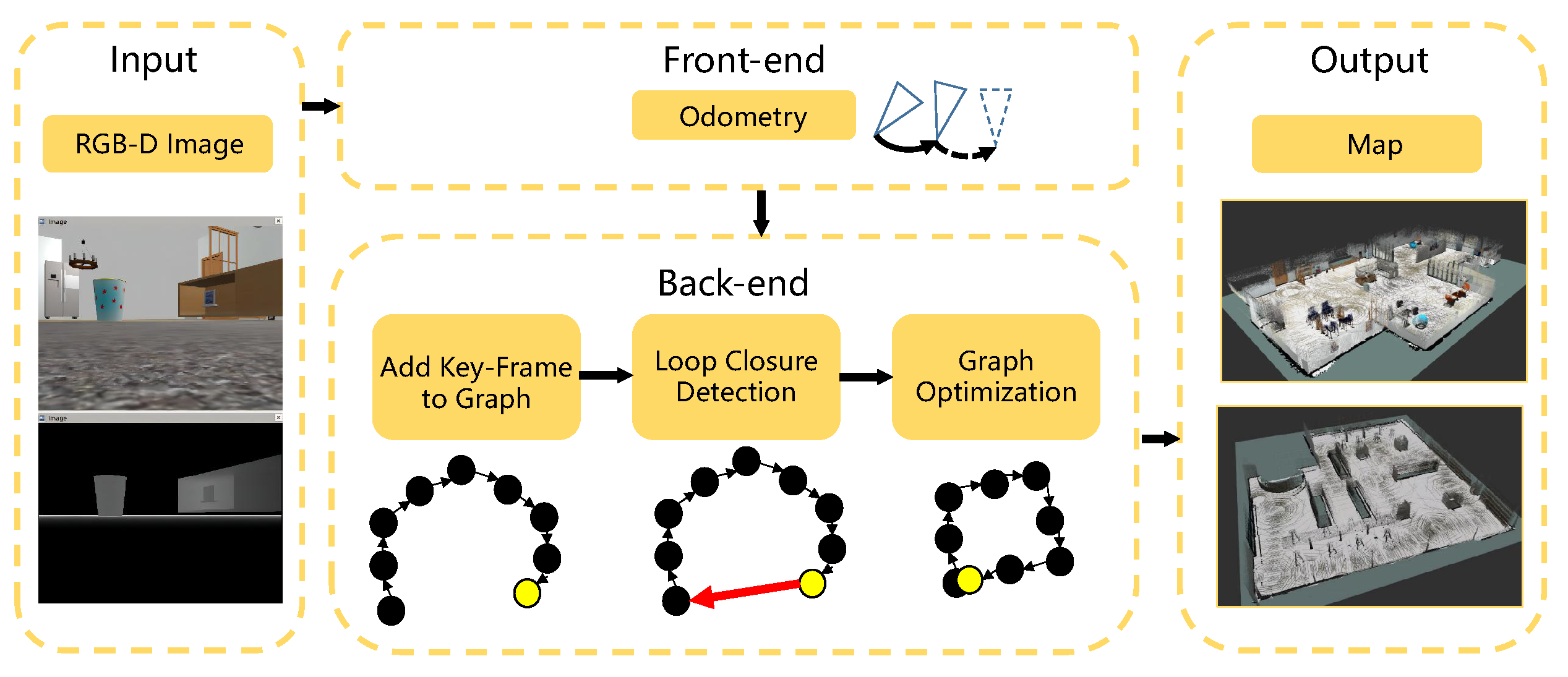
Figure 3.
Multi-line LiDAR-based SLAM system structure diagram.
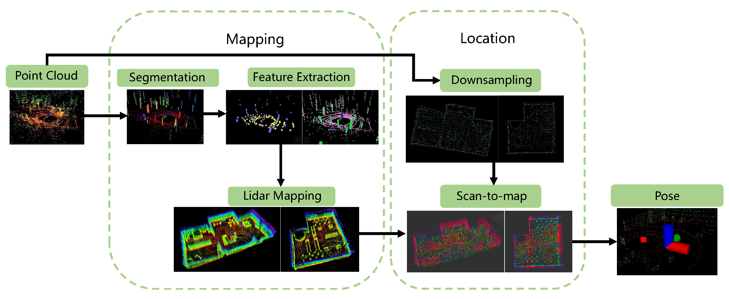
Figure 4.
Two-wheel differential robot model.
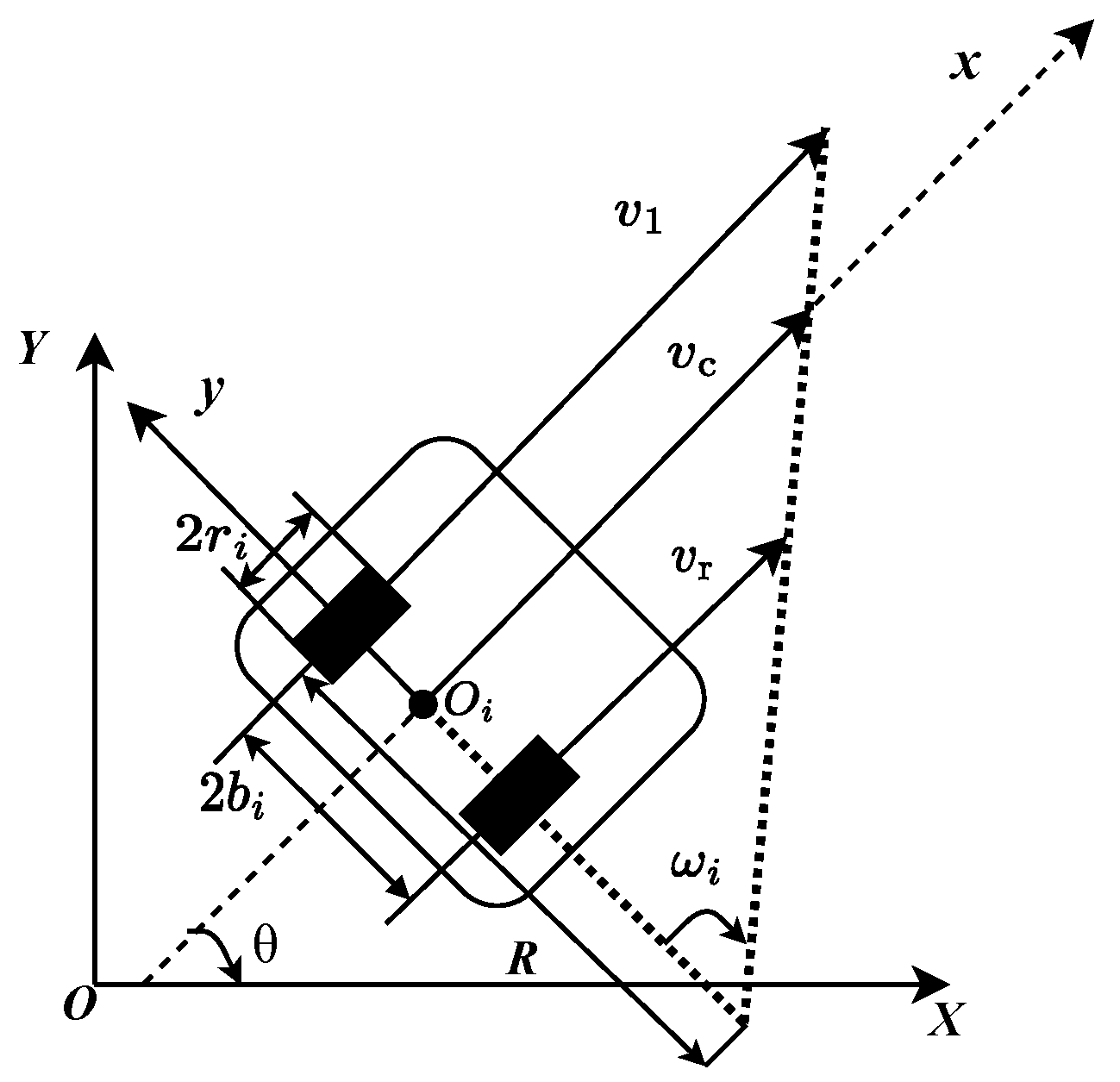
Figure 5.
Time interval and pose sequence of the TEB.
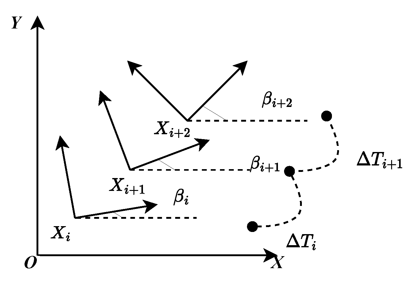
Figure 6.
Hybrid path planning algorithm flow chart.
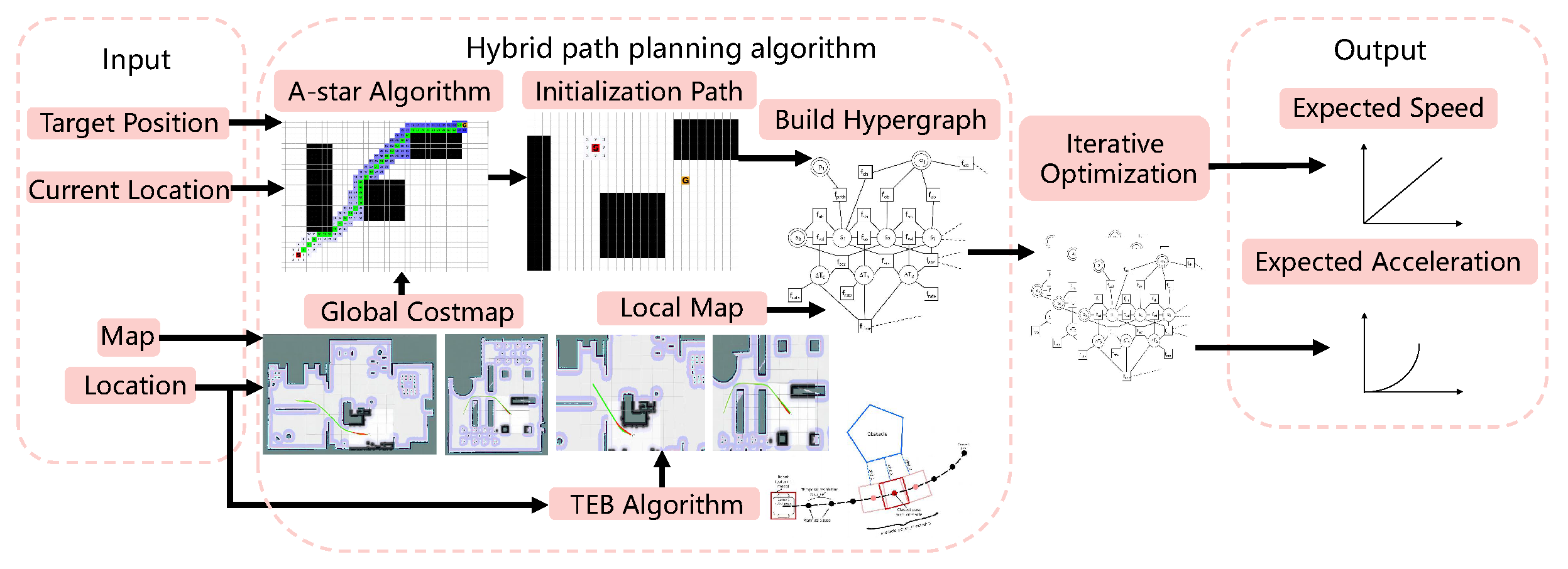
Figure 7.
Simulation environment.(a)House scene;(b)Library scene.
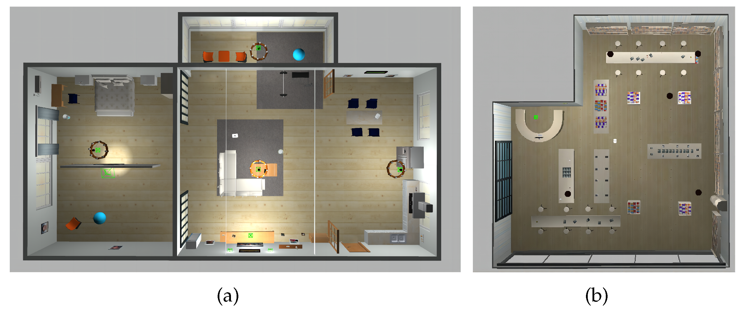
Figure 8.
Vision-based mapping results.(a)House scene;(b)Library scene.
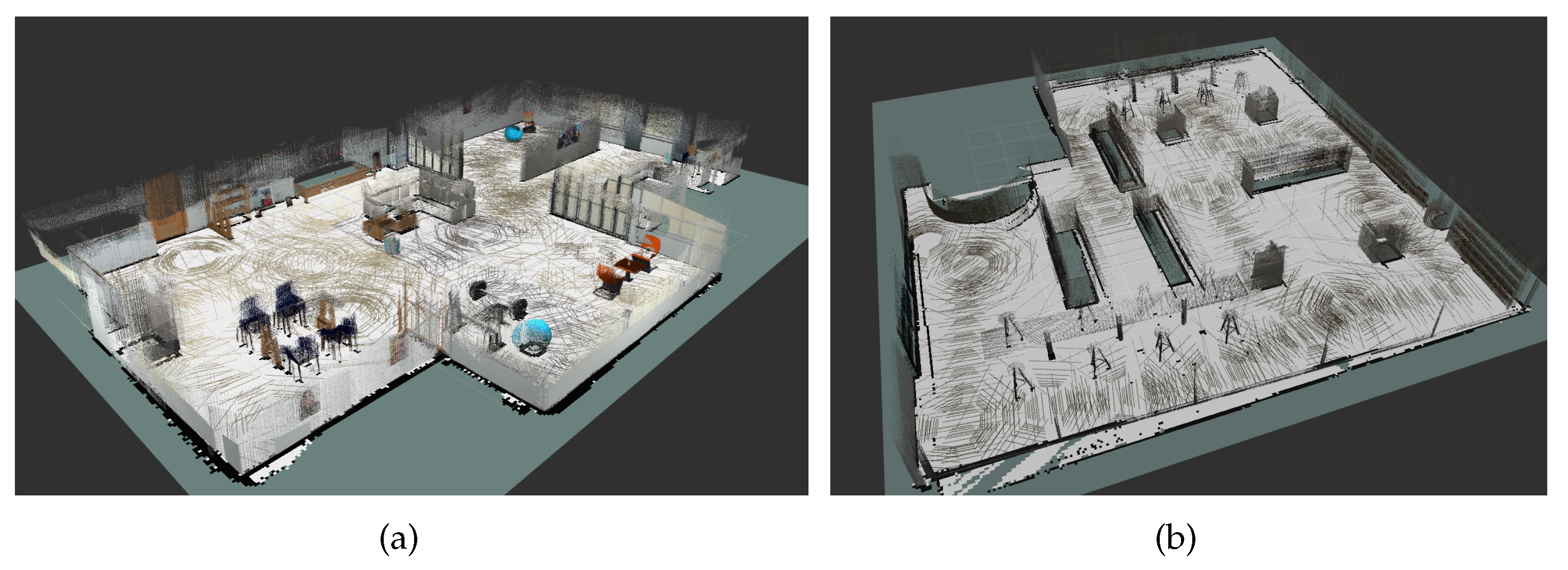
Figure 9.
Laser-based mapping results.(a)House scene;(b)Library scene.
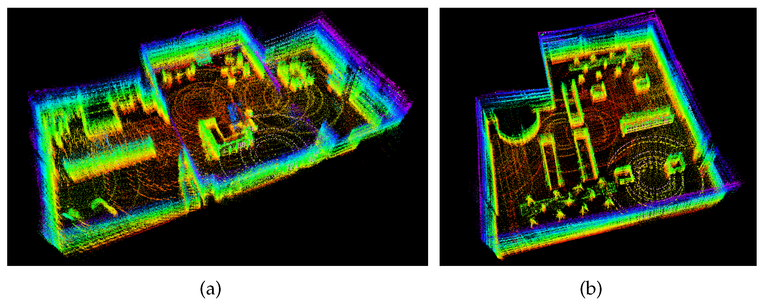
Figure 10.
Local path planning map.(a)House scene;(b)Library scene.
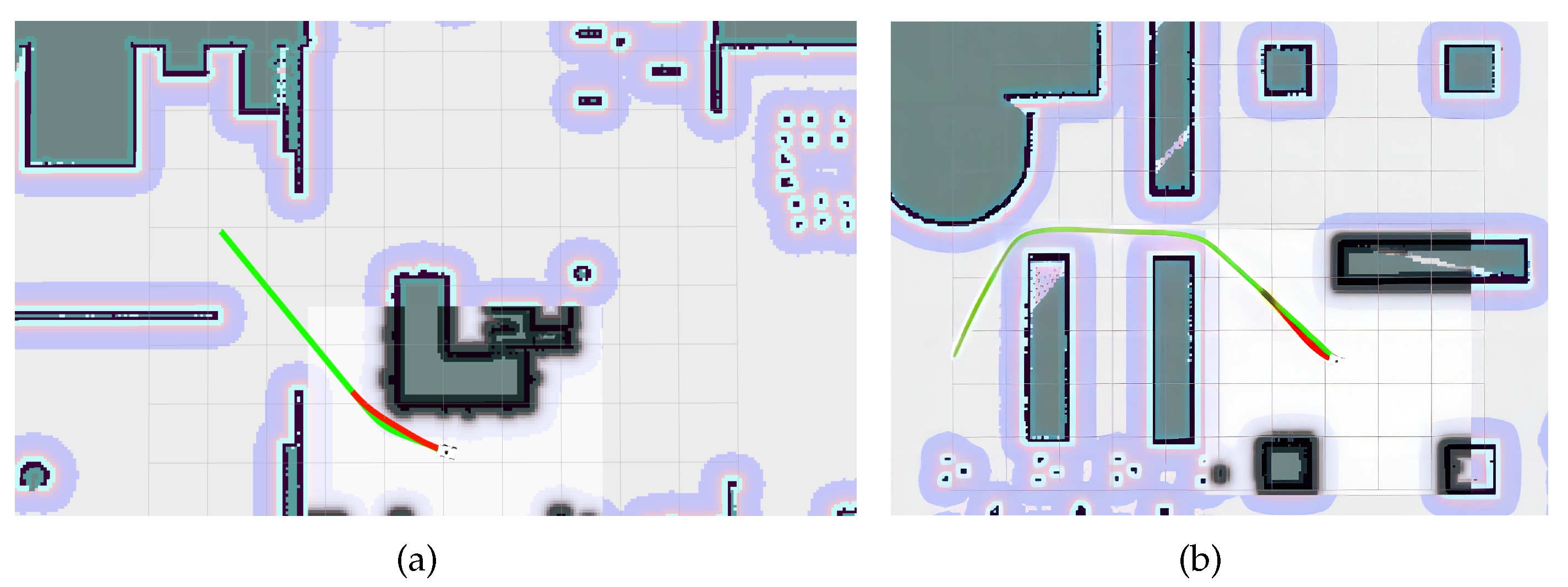
Figure 11.
Global path planning map.(a)House scene;(b)Library scene.
Disclaimer/Publisher’s Note: The statements, opinions and data contained in all publications are solely those of the individual author(s) and contributor(s) and not of MDPI and/or the editor(s). MDPI and/or the editor(s) disclaim responsibility for any injury to people or property resulting from any ideas, methods, instructions or products referred to in the content. |
© 2023 by the authors. Licensee MDPI, Basel, Switzerland. This article is an open access article distributed under the terms and conditions of the Creative Commons Attribution (CC BY) license (http://creativecommons.org/licenses/by/4.0/).
Copyright: This open access article is published under a Creative Commons CC BY 4.0 license, which permit the free download, distribution, and reuse, provided that the author and preprint are cited in any reuse.
Submitted:
11 April 2023
Posted:
11 April 2023
You are already at the latest version
Alerts
A peer-reviewed article of this preprint also exists.
This version is not peer-reviewed
Submitted:
11 April 2023
Posted:
11 April 2023
You are already at the latest version
Alerts
Abstract
Factory safety inspections are crucial for ensuring safe production. However, manual inspections present issues such as low efficiency and high workload. Inspection robots provide an efficient and reliable solution for completing patrol tasks. The development of robot localization and path planning technologies provides guarantees for factory inspection robots to autonomously complete inspection tasks in complex environments. This paper studies mapping and localization, as well as path planning methods for robots in order to meet the application requirements of factory inspections. Two SLAM application systems based on multiple-line laser radar and vision are designed for different scenarios in consideration of the limitations of cameras and laser sensors in terms of their own characteristics and applicability in different environments. To address the issue of low efficiency in inspection tasks, a hybrid path planning algorithm that integrates the A-star algorithm and time elasticity band algorithm is proposed. This algorithm effectively solves the problem of path planning in complex environments that is prone to falling into local optimal solutions, thereby improving the inspection efficiency of robots. Experimental tests show that the designed SLAM and path planning methods can meet the needs of robot inspection in complex scenes and have good reliability and stability. The code used in this article is open source and can be accessed at https://github.com/Mxiii99/RSPP_CS.git.
Keywords:
Subject: Computer Science and Mathematics - Robotics
1. Introduction
With the introduction of "Industry 4.0", robotics technology has rapidly advanced. Among them, inspection robots have been extensively used in aerospace, manufacturing, agriculture, service industries, and other fields due to their superior flexibility, mobility, and functionality [1,2]. As inspection application scenarios become more diversified and complex, higher requirements are placed on the autonomous navigation performance of robots. Robot navigation technology mainly consists of SLAM technology and path planning technology. Simultaneous Localization and Mapping (SLAM) is the process by which a mobile robot determines its own position and creates a map through sensors carried in the surrounding environment. Path planning technology creates the optimal navigation path for the robot to reach the target location based on different task goals and requirements.
SLAM technology can be classified into two categories based on different sensors: vision-based and LIDAR-based. The MonoSLAM method proposed by Davison et al. estimates the camera pose by extracting sparse feature points frame by frame, which is the first real-time visual SLAM system using a single camera [3]. Subsequently, Klein et al. proposed the PTAM method, which introduced nonlinear optimization and keyframe mechanism [4], solving the problem of high computational complexity in MonoSLAM. Newcombe et al. proposed a dense per-pixel method based on RGB-D camera, which can achieve real-time tracking and reconstruction [5]. As for LIDAR-based SLAM methods, Grisetti et al. proposed a 2D SLAM algorithm based on particle filtering, which solved the problem of particle dissipation caused by resampling through reducing the number of particles [6]. Konolige et al. proposed the first open-source algorithm based on graph optimization by using highly optimized and non-iterative square-root factorization to sparsify and decouple the system [7]. Kohlbrecher et al. designed the Hector SLAM algorithm, which matches the current frame’s LIDAR data with the factor graph and optimizes the pose using the Gauss-Newton method to obtain the optimal solution and bias [8].
Path planning is to plan a collision-free optimal path from the starting point to the destination point in the map environment. Path planning can be divided into global and local path planning according to whether the environment information is known in advance. Dijkstra et al. proposed the shortest path planning algorithm, which uses breadth-first search to search for paths [9]. Hart et al. proposed the A-star algorithm, which reduces the search nodes by using heuristic evaluation function and improves the efficiency of path searching [10]. Fox et al. proposed the DWA, which samples velocity dynamically in the robot’s sampling space according to the robot’s kinematic model and current motion parameters, and selects the best trajectory [11]. To address the insufficient evaluation function of DWA, Chang et al. proposed an improved DWA algorithm based on Q-learning, which modifies and extends the evaluation function and adds two evaluation functions to improve navigation performance and achieve higher navigation efficiency and success rate in complex unknown environments [12]. Rösmann et al. proposed the Time Elastic Band algorithm based on multi-objective optimization, which ensures that the robot can output a smooth trajectory under the premise of satisfying its kinematic constraints [13].
Both lidar and camera sensors are essential for factory inspections, but their applicability depends on the specific application scenarios and factory environments. Lidar is suitable for long-distance and high-precision measurements, such as inventory management in large warehouses and position control in robot operations. However, lidar has limitations in processing details and colors, making it unsuitable for high-visual requirements scenes. Camera sensors, with their functions such as image recognition, detection, and tracking, are ideal for environments that require high-precision visual detection and recognition, such as detecting product dimensions, shapes, colors, and performing automated visual inspections during assembly processes on production lines. In addition, camera sensors have strong processing capabilities for details and colors, providing more detailed image information. However, camera sensors are highly dependent on ambient light, which can limit their effectiveness in poor lighting conditions or when obstacles are present.
In this article, we designed two sets of SLAM systems based on multi-line lidar and vision sensors respectively to meet the inspection needs of robots in different environments. Global path planning using the A-star algorithm was adopted to improve navigation efficiency and help robots quickly plan the optimal path, reducing inspection time and costs. However, the A-star algorithm is not suitable for dynamic environments. Therefore, we introduced the Time Elastic Band algorithm, a real-time path planning algorithm that can adapt to changes in the environment and obstacles, resulting in more optimized path planning results to improve the efficiency of robot inspections and reduce collisions and other safety issues between robots and factory equipment. The method proposed in this article adopts a global and local fusion path planning algorithm for both lidar SLAM and vision SLAM, ultimately achieving autonomous navigation and obstacle avoidance of inspection robots in comple.
Figure 1.
System framework.
2. Inspection robot SLAM system
2.1. Visual-SLAM Algorithm Design and Implementation
In the factory environment, the position and motion of inspection robots and equipment may undergo rapid changes, thus requiring real-time acquisition and processing of sensor data for accurate localization and mapping. To achieve this, we have chosen an appearance-based localization and mapping method that is invariant to time and scale, as shown in the structural diagram in Figure 2.
From Figure 2, it can be seen that RGB-D images are used as external input, and the ORB algorithm is used to extract feature points from RGB-D images [14]. Then, a Bag-of-Words based image matching method is used to match feature points between adjacent frames. The loop-closure detection mechanism is introduced to eliminate drift. When the robot returns to an area previously visited, the loop-closure detection can identify the area and match the newly observed data with the previous map data, thus addressing the cumulative drift problem. Next, graph optimization is performed, where the robot’s poses are represented as nodes in the graph and the observed data is represented as edges. Then, the least squares method is used to optimize the positions of all nodes, minimizing the error between observed and predicted data. Finally, a dense map can be generated.
This vision-based mapping and localization algorithm utilizes global and local loop-closure detection techniques, which can identify and handle errors and drift in sensor data, improving the robustness and accuracy of localization and mapping, and enhancing the efficiency and real-time performance of inspection robots.
2.2. Multi-line LiDAR-based SLAM Algorithm Design and Implementation
In indoor factory environments, lighting conditions can vary with time and location, which may lead to misidentification of objects or inaccurate positioning by visual sensors. However, laser sensors do not require an external light source, as they emit their own laser beams and are not affected by lighting issues. Therefore, we have adopted a lightweight and ground optimized laser odometry and mapping method, whose structural diagram is shown in Figure 3. Firstly, the laser point cloud data is dimensionally reduced, projecting the 3D laser onto a 2D depth image, segmenting the ground according to the pitch angle, clustering non-ground point clouds, and obtaining labeled point cloud data. Then, feature extraction is performed based on smoothness, resulting in four sets of feature point clouds. Constraint relationships are established for the feature point cloud sets, and the 6-DOF pose transformation matrix is solved using the Levenberg-Marquardt (LM) optimization method. Subsequently, loop detection is conducted using the Iterative Closest Point (ICP) algorithm, and finally, the current point cloud is mapped to the global map based on graph optimization, completing the establishment of a high-precision map [15].
1) Point cloud segmentation: Due to the complexity of the inspection environment and other factors, noise may exist in the laser point cloud data. We first use point cloud segmentation to filter out noise. By projecting a frame of 3D point cloud onto a 2D depth image using a projection method, ground segmentation is performed to separate non-ground points [16]. Let be the point cloud data obtained by the lidar at time t, where is a point in . These points are projected onto a depth image, and the 3D points in space become 2D pixels in space. After projection, the Euclidean distance of point to the sensor is obtained. Since the 3D point cloud contains a large amount of ground information, it is necessary to filter the point cloud to improve the efficiency and accuracy of feature extraction. Firstly, the ground points are labeled, and the labeled ground points will no longer be segmented in subsequent steps. After separating ground points and non-ground points, the non-ground points are processed by clustering. After this module, each point has its own segmentation label (ground or non-ground), row and column indices in the depth image, and the Euclidean distance to the sensor.
2)Feature extraction: According to the smoothness, the projected depth image is horizontally divided into several sub-images. For each sub-image, the following process is performed [17]: Let S be the set of continuous points in the same row in the depth image, and calculate the smoothness c of point .
where and are the Euclidean distances from points and to the sensor. According to Equation (1), the smoothness of each point can be calculated, and then the smoothness is sorted. After sorting, feature points are selected. Different types of features are segmented based on the set threshold . The edge points with a smoothness c greater than are selected as set , and the plane points with a smoothness c less than are selected as set . The largest edge points with the maximum c value and the smallest plane points with the minimum c value are selected from all sub-images to form the edge feature point set and the plane feature point set . Then, edge points not belonging to ground points with the maximum c value are selected from set to form set , and plane points belonging to ground points with the minimum c value are selected from set to form set . Obviously .
3)Radar Odometry: The odometry module estimates the robot’s pose change between adjacent frames using a radar sensor. In the estimation process, tag matching is used to narrow down the matching range and improve accuracy, and a two-step LM optimization method is used to find the transformation relationship between two consecutive frames [18]. The first step uses ground feature points to obtain , and the second step matches the edge features extracted from the segmented point cloud to obtain the transformation . Finally, by fusing and , a 6-DOF pose transformation matrix is obtained.
4)Radar Mapping: After obtaining the pose change between adjacent frames with radar odometry, the features in the feature set at time t are matched with the surrounding point cloud to further refine the pose transformation. Then, using the LM optimization, the final transformed pose is obtained and the pose graph is sent to GTSAM for map optimization to update the sensor estimated pose and the current map [19].
In addition, noise may exist in the collected laser point cloud data. In order to achieve high-precision localization on the map, it is necessary to preprocess the high-precision map. We use a statistical-based robust filter to remove outliers, a pass-through filter to clip the point cloud within a specified coordinate range, and a voxel grid filter to downsample the point cloud. For the inspection task that requires high-precision real-time localization, we perform real-time localization on the constructed high-precision map through point cloud registration. First, the reference point cloud (i.e., high-precision map) is transformed into a multivariate normal distribution [20]. If the transformation parameters can accurately match the reference point cloud and the current point cloud, the transformed points in the reference frame have a high probability density. Therefore, an optimization method can be used to calculate the transformation parameters that maximize the sum of the probability densities. In this case, the two sets of laser point cloud data match best. The specific algorithm steps are as follows:
1) Given the current scanning point cloud S and the reference point cloud T, the space occupied by the T point cloud is divided into voxel grids of a specified size, and the expected vector and covariance matrix of N points in each voxel grid are calculated.
Here, represents the three-dimensional coordinates of the point cloud in the voxel grid.
2) Initialize the transformation parameters to be solved, with zero values or odometry data. For each sample in the S point cloud, transform it to the T point cloud according to the transformation parameters. Let be the coordinate of in the T point cloud coordinate system. Find the grid where falls in the T point cloud, and combine the probability density function of each grid in the T point cloud to calculate the corresponding probability distribution function .
3) Add up the probability densities calculated for each mapped point to obtain the registration score.
Use the Newton optimization algorithm to optimize the objective function until the optimal transformation parameters are found that maximize the registration score, complete convergence, and solve the best rigid body transformation between the target and source point clouds to achieve accurate localization.
3. Inspection robot Path planning system
3.1. Sports model
Currently, the chassis of inspection robots mainly consists of legged, tracked, and wheeled types, each with its advantages and disadvantages in different environments. Legged inspection robots have strong terrain adaptability, but their structure and control system are complex. Tracked inspection robots have high traction and strong applicability in complex terrains such as outdoor, sandy, and muddy areas, but their speed is relatively low, and they have high motion noise. Wheeled inspection robots have fast speed, high efficiency, and low motion noise, and are widely used. In this paper, we focus on the complex indoor factory environment and adopt a two-wheel differential wheeled robot whose kinematic model is shown in Figure 4 [21].
In Figure 4, the motion of robot is completed by two independently driven wheels. Let the radius of the driving wheel be , and define the midpoint of the two driving wheels as . The distance between the two wheels is , where is the inertial Cartesian coordinate system, and is the local coordinate system of the robot. is the speed of the left driving wheel, is the speed of the right wheel, and is the speed of the center of the robot. If , the angular velocity can be obtained. According to the robot model, the forward speed depends on the speed of the wheels.
The angular velocity is determined by the difference in speed between the left and right driving wheels and the distance between them.
In the ideal case, according to the principle of rigid motion, the trajectory of the robot is a circle, and the radius can be expressed as
The kinematic equation of the robot can be expressed as
The above formula is the pose state matrix and motion state matrix, and the final formula can be written as follows:
where is a smooth linearly independent matrix, and V is the motion matrix of the robot.
3.2. Path Planning
The path planning of inspection robots mainly relies on the constructed grid map to generate a safe and collision-free path by specifying the start and target locations. The path planning for robots can be divided into global path planning and local path planning.
(1) Global path planning
To ensure that the patrol robot can effectively avoid obstacles globally and locally, and considering that the grid map of the actual road scene is relatively simple, the A-star algorithm is used as the global path planning method to provide accurate obstacle avoidance directions for the robot through real-time planning [22,23]. A-star combines heuristic search with breadth-first algorithm to select the search direction through the cost function , and expands around the starting point. The cost value of each surrounding node is calculated by the heuristic function , and the minimum cost value is selected as the next expanding point. This process is repeated until the endpoint is reached, generating a path from the starting point to the endpoint. In the search process, since each node on the path is the node with the minimum cost, the cost of the path obtained is also minimum. The cost function of the A-star algorithm is
where is the cost function at the current position, is the cost value from the starting position to the current position in the search space, and is the cost value from the current position to the goal position. In the A-star algorithm, the selection of the heuristic function is crucial. Since the map environment is a grid map with obstacles, the Manhattan distance is used as the heuristic function, which is given by:
where , represent the coordinates from the current position to the target position. In the path planning of the A-star algorithm, the nodes are stored in two lists, Closelist and Openlist. The nodes that have been searched and generated cost values are stored in Openlist. The node with the minimum estimated cost is stored in Closelist, and the moving trajectory is formed by processing the trajectories of each node in Closelist. The specific steps are as follows:
Step 1.The starting point s of the robot is the first calculated point, and the surrounding nodes are added to Openlist, and the cost function of each point is calculated.
Step 2.Search Openlist, select the node with the smallest cost value as the current processing node n, remove the node from Openlist, and put it into Closelist.
Step 3.If the real cost value of the adjacent node from the current processing node to the starting point s is smaller than the original value, the parent node of the adjacent node is set to the current processing node; if it is larger, the current processing node is removed from Closelist, and the node with the second smallest value of is selected as the current processing node.
Step 4.Repeat the above steps until the target point g is added to Closelist, traverse along each parent node, and the obtained node coordinates are the path.
(2)Local path planning
The working environment of inspection robots is not always static. In the process of moving along the global path, real-time obstacles may appear. To avoid collisions, the Timed-Elastic-Band (TEB) algorithm, which introduces local path planning with time elasticity, is used on the basis of global path planning to achieve real-time obstacle avoidance [24]. The TEB algorithm is an optimization algorithm that follows the path generated by the global path planner. The local trajectory it generates is composed of a series of continuous time and pose sequences, and the robot’s pose is defined as:
where represents the i-th pose in the robot coordinate system, including position information , and angle . The time interval between adjacent poses and is denoted by , as shown in Figure 5.
In the optimization process, the TEB algorithm applies graph optimization to the adjacent time intervals and states of the robot as nodes, and uses velocity, acceleration, and non-holonomic constraints of the robot as edges. It also considers obstacle information, discrete interval of planned trajectory, and adjacent temporal and spatial sequence constraints. Finally, the G2O solver is used to calculate the control variable (where v and represent the linear and angular velocity of the robot, respectively), to obtain the optimal trajectory. The TEB algorithm obtains the optimal pose points through weighted multi-objective optimization [25,26], where the mathematical description of the objective function is:
where is the objective function that considers various constraints, is the constraint function, is the weight of each item, and is the optimal TEB trajectory. The TEB algorithm has four constraint functions.
1) Path following and obstacle constraint objective function
The TEB algorithm aims to avoid collisions with static or dynamic obstacles while following the path. The algorithm treats piecewise continuous and differentiable functions as constraints and punishes behaviors that do not conform to the constraints. Specifically:
Building on Equation (18), penalty functions and are constructed. Here, denotes the boundary, is the offset factor, S is the scaling factor, n is the order, is the independent variable representing the distance between the path point and obstacle, is the maximum distance of the trajectory deviation from the path point, and is the minimum distance between the trajectory and obstacle.
2) The velocity and acceleration constraint functions of a robot
According to the dynamic equation, the constraint functions of the robot’s velocity and acceleration are expressed as equations (21) - (24) :
Linear velocity:
Angular velocity:
Linear acceleration:
Angular acceleration:
3) Non-holonomic constraint:
The robot used in the algorithm simulation and experiment is a differential drive structure with two degrees of freedom, which cannot perform translational motion along the y-axis of the robot coordinate system. The curvature of the circular arc between two adjacent robot poses is approximately constant, and the outer product of the direction vector and the turning angle between adjacent poses in the robot coordinate system is equal to the outer product of the turning angle and the direction vector . represents the orientation of the robot in the global coordinate system, and the corresponding relationship equation and non-holonomic constraint are:
The objective function punishes the quadratic error for violating this constraint, ensuring that the output velocity of the robot follows the non-holonomic constraint.
4) Fastest path constraint
The TEB algorithm incorporates the time interval information between poses, and the total time is the sum of all time intervals. The relevant objective function is:
After optimizing the TEB sequence, the objective function of the constraints is optimized to ensure that the path planned by the algorithm achieves the best results in terms of obstacle avoidance, time, and distance.
(3)Path planning based on fusion algorithm
The A-star algorithm yields a navigation path consisting of only the start point, key points, and destination point, but it cannot avoid unknown obstacles in the environment. The TEB algorithm exhibits good local obstacle avoidance ability, but with only a single final goal point as a guide, it is prone to becoming trapped in local optima. Therefore, we propose a hybrid path planning algorithm that combines the strengths of both algorithms. The specific algorithm process is shown in Figure 6.
Global path planning takes a static obstacle cost map as input, and does not consider the robot’s mechanical performance and kinematic constraints when planning the path. It uses the A-star algorithm to plan the optimal path from the robot’s current position to the desired target position, and provides an initial value for local planning.
Local path planning collects path nodes on the global optimal path, and optimizes the global path subset between the robot’s current node and the collected path nodes. It combines the static obstacle cost map and dynamic obstacle cost map, and uses the TEB algorithm to continuously adjust the pose and orientation of the robot during its movement, taking into account its shape, dynamic model, and motion performance in the scope of local planning. When encountering dynamic obstacles, it removes the old robot pose and adds a new robot pose, so that a new path can be generated in each iteration, and an optimized path can be obtained through continuous iteration.
By fusing navigation algorithms, we achieve optimal global path planning and real-time obstacle avoidance functionality in the process of mobile robot navigation.
4. Experiment and Analysis
4.1. Experiment settings
In order to verify the effectiveness of navigation systems in practical applications, we conducted experiments using a Turtlebot3 mobile robot in different types of scenarios built using the Gazebo simulation platform within the ROS on a 64-bit Ubuntu 18.04 operating system with 4GB of running memory. As shown in Figure 7, we constructed a home environment and a library environment to simulate real-world environments. Using the real-time localization and mapping capabilities in Rviz, we scanned the simulated environments, constructed corresponding maps, and performed path planning.
4.2. Performance evaluation
4.2.1. Visual-SLAM Algorithm performance evaluation
This paper presents a method for constructing a corresponding point cloud map using a depth camera in a ROS environment. The depth camera data is first read in the ROS environment, and then the front-end and back-end threads are executed to construct a sparse feature point map, which is continuously updated to create a real-time point cloud map. Keyframes from the front-end are passed into the point cloud construction thread to generate the point cloud map. The effectiveness of the proposed algorithm for generating maps is validated by the corresponding point cloud map in Figure 8, which demonstrates good 3D effects for constructing maps in indoor environments. As shown in Figure 8, the algorithm detects the object’s motion trajectory, which is consistent with the actual trajectory. Although there are deviations between the detected trajectory and the actual trajectory, there is no serious deviation, which satisfies the perception requirements of the robot. When the object’s motion trajectory changes significantly, there is still no serious deviation, which also meets the perception requirements of the robot.
4.2.2. Multi-line LiDAR-based SLAM Algorithm performance evaluation
From the comparison between point cloud mapping and visual mapping, it can be observed that maps constructed using multi-line laser scanning are clearer than those constructed using visual algorithms, which reduces accumulated errors and provides better handling of edge contours. Furthermore, a comparison was conducted on mapping time, mapping effectiveness, and CPU utilization, in order to validate the feasibility, reliability, and accuracy of the algorithm.
To ensure the accuracy of the experiments, multiple tests were conducted. The robot was fixed at a certain position, denoted as the origin (0,0), and the output object motion data was compared with the actual object motion data. The results are shown in Figure 9. The algorithm detected that the point cloud map was generally consistent with the simulated scene, and that the detected trajectory was not significantly deviated from the actual trajectory, which satisfies the perception requirements of the robot. As shown in the figure, when there were large changes in the object’s motion trajectory, there was a slight deviation between the detected trajectory and the actual trajectory, but no serious deviation occurred, which still satisfied the perception requirements of the robot.
4.2.3. Path Planning Performance Evaluation
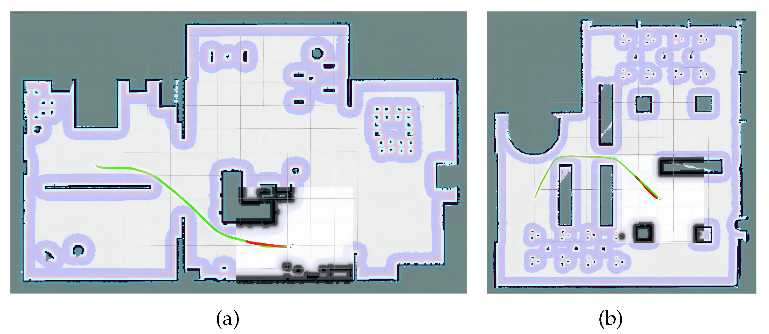
Through testing, the path distance planned by the A-star algorithm has a certain distance from the obstacles, which avoids the collision of the robot. At the same time, global path planning has a good effect and can accurately reach the set target point location, satisfying the requirement of precise navigation. The robot moves along a square path. When encountering obstacles, it autonomously avoids them through local path planning. The process and result of local path planning are shown in Figure 10. After configuring the relevant parameters, observe the 3D view area of robot navigation in Rviz. The environment of the map is displayed as a global cost map, and the environment around the robot is a local cost map. The blue area is the expansion layer of the obstacle, which is expanded outward on the map to avoid collision between the robot and the obstacle. By adding the Path plugin in RViz, you can see the path that the robot moves. The green line is the route of global path planning, and the red line is the route of local path planning. It can be seen from Figure 10 that the local path planning route of the inspection robot is smooth and the planned route does not enter the expansion layer of the obstacle, which can reasonably avoid the surrounding obstacles and has a good obstacle avoidance effect. The global path planning is shown in Figure 11. After testing, the inspection robot can accurately achieve autonomous obstacle avoidance and complete local path planning for the set target point, satisfying the requirement of precise navigation.
5. Conclusions
The utilization of intelligent inspection robots has been shown to enhance production efficiency and reduce costs. However, the complex factory environment, filled with machinery equipment, pipelines, cables, and other obstacles, can pose a challenge to accurate inspections. To address this, we have developed a high-precision navigation inspection system that is specifically designed for complex factory scenes. The system is equipped with two types of sensors, visual and LiDAR, to allow for rich environmental information and localization and mapping. Optimal path planning is achieved by combining the A-star algorithm and TEB algorithm for dynamic programming. To evaluate the performance of the navigation system, simulations were conducted in two scenarios using Gazebo simulation software in the ROS system: a residential area and a library. Results indicate that the navigation system provides real-time localization and map construction, can navigate mobile platforms, and implements real-time obstacle avoidance in different scenarios. As such, this technology can be applied to the localization and navigation system of wheeled inspection robots in various complex environments, and has significant reference value.
Author Contributions
Conceptualization, X.M. and X.W.; methodology, X.M. and X.W.; software, X.M. and X.W.; validation, X.M., X.W. and Z.L. All authors have read and agreed to the published version of the manuscript.
Funding
This research is funded by the Graduate Education and Teaching Quality Improvement Project of Beijing University of Architecture and Architecture (J2023017); the Lecturer Support Plan Project of Beijing University of Architecture and Architecture (YXZJ20220804); the Open Project of Anhui Provincial Key Laboratory of Intelligent Building and Building Energy Efficiency, Anhui Jianzhu University (IBES2020KF06); the BUCEA Post Graduate Innovation Project.
Informed Consent Statement
For studies not involving humans or animals.
Data Availability Statement
Not applicable.
Acknowledgments
Not applicable.
Conflicts of Interest
The authors declare no conflict of interest.
References
- Bahrin, M.A.K.; Othman, M.F.; Azli, N.H.N.; Talib, M.F. Industry 4.0: A review on industrial automation and robotic. Jurnal teknologi 2016, 78. [Google Scholar]
- Choi, H.; Ryew, S. Robotic system with active steering capability for internal inspection of urban gas pipelines. Mechatronics 2002, 12, 713–736. [Google Scholar] [CrossRef]
- Davison, A.J.; Reid, I.D.; Molton, N.D.; Stasse, O. MonoSLAM: Real-time single camera SLAM. IEEE transactions on pattern analysis and machine intelligence 2007, 29, 1052–1067. [Google Scholar] [CrossRef] [PubMed]
- Pire, T.; Fischer, T.; Castro, G.; De Cristóforis, P.; Civera, J.; Berlles, J.J. S-PTAM: Stereo parallel tracking and mapping. Robotics and Autonomous Systems 2017, 93, 27–42. [Google Scholar] [CrossRef]
- Zhou, H.; Ummenhofer, B.; Brox, T. DeepTAM: Deep tracking and mapping with convolutional neural networks. Springer, 2020, Vol. 128, pp. 756–769.
- Grisetti, G.; Kümmerle, R.; Stachniss, C.; Burgard, W. A tutorial on graph-based SLAM. IEEE Intelligent Transportation Systems Magazine 2010, 2, 31–43. [Google Scholar] [CrossRef]
- Strasdat, H.; Davison, A.J.; Montiel, J.M.; Konolige, K. Double window optimisation for constant time visual SLAM. 2011 international conference on computer vision. IEEE, 2011, pp. 2352–2359.
- Harik, E.H.C.; Korsaeth, A. Combining hector slam and artificial potential field for autonomous navigation inside a greenhouse. Robotics 2018, 7, 22. [Google Scholar] [CrossRef]
- Noto, M.; Sato, H. A method for the shortest path search by extended Dijkstra algorithm. Smc 2000 conference proceedings. 2000 ieee international conference on systems, man and cybernetics.’cybernetics evolving to systems, humans, organizations, and their complex interactions’(cat. no. 0. IEEE, 2000, Vol. 3, pp. 2316–2320.
- Seet, B.C.; Liu, G.; Lee, B.S.; Foh, C.H.; Wong, K.J.; Lee, K.K. A-STAR: A mobile ad hoc routing strategy for metropolis vehicular communications. Networking 2004: Networking Technologies, Services, and Protocols; Performance of Computer and Communication Networks; Mobile and Wireless Communications Third International IFIP-TC6 Networking Conference Athens, Greece, –14, 2004, Proceedings 3. Springer, 2004, pp. 989–999. 9 May.
- Ogren, P.; Leonard, N.E. A convergent dynamic window approach to obstacle avoidance. IEEE Transactions on Robotics 2005, 21, 188–195. [Google Scholar] [CrossRef]
- Chang, L.; Shan, L.; Jiang, C.; Dai, Y. Reinforcement based mobile robot path planning with improved dynamic window approach in unknown environment. Autonomous Robots 2021, 45, 51–76. [Google Scholar] [CrossRef]
- Rösmann, C.; Hoffmann, F.; Bertram, T. Timed-elastic-bands for time-optimal point-to-point nonlinear model predictive control. 2015 european control conference (ECC). IEEE, 2015, pp. 3352–3357.
- Ragot, N.; Khemmar, R.; Pokala, A.; Rossi, R.; Ertaud, J.Y. Benchmark of visual slam algorithms: Orb-slam2 vs rtab-map. 2019 Eighth International Conference on Emerging Security Technologies (EST). IEEE, 2019, pp. 1–6.
- Yang, J.; Wang, C.; Luo, W.; Zhang, Y.; Chang, B.; Wu, M. Research on point cloud registering method of tunneling roadway based on 3D NDT-ICP algorithm. Sensors 2021, 21, 4448. [Google Scholar] [CrossRef] [PubMed]
- Xue, G.; Wei, J.; Li, R.; Cheng, J. LeGO-LOAM-SC: An Improved Simultaneous Localization and Mapping Method Fusing LeGO-LOAM and Scan Context for Underground Coalmine. Sensors 2022, 22, 520. [Google Scholar] [CrossRef] [PubMed]
- Zheng, X.; Gan, H.; Liu, X.; Lin, W.; Tang, P. 3D Point Cloud Mapping Based on Intensity Feature. Artificial Intelligence in China: Proceedings of the 3rd International Conference on Artificial Intelligence in China. Springer, 2022, pp. 514–521.
- Zhang, G.; Yang, C.; Wang, W.; Xiang, C.; Li, Y. A Lightweight LiDAR SLAM in Indoor-Outdoor Switch Environments. 2022 6th CAA International Conference on Vehicular Control and Intelligence (CVCI). IEEE, 2022, pp. 1–6.
- Karal Puthanpura, J. ; others. Pose Graph Optimization for Large Scale Visual Inertial SLAM 2022. [Google Scholar]
- Li, H.; Dong, Y.; Liu, Y.; Ai, J. Design and Implementation of UAVs for Bird’s Nest Inspection on Transmission Lines Based on Deep Learning. Drones 2022, 6, 252. [Google Scholar] [CrossRef]
- Moshayedi, A.J.; Roy, A.S.; Sambo, S.K.; Zhong, Y.; Liao, L. Review on: the service robot mathematical model. EAI Endorsed Transactions on AI and Robotics 2022, 1. [Google Scholar] [CrossRef]
- Zhang, B.; Li, G.; Zheng, Q.; Bai, X.; Ding, Y.; Khan, A. Path planning for wheeled mobile robot in partially known uneven terrain. Sensors 2022, 22, 5217. [Google Scholar] [CrossRef] [PubMed]
- Vagale, A.; Oucheikh, R.; Bye, R.T.; Osen, O.L.; Fossen, T.I. Path planning and collision avoidance for autonomous surface vehicles I: a review. Journal of Marine Science and Technology.
- Gul, F.; Mir, I.; Abualigah, L.; Sumari, P.; Forestiero, A. A consolidated review of path planning and optimization techniques: Technical perspectives and future directions. Electronics 2021, 10, 2250. [Google Scholar] [CrossRef]
- Wu, J.; Ma, X.; Peng, T.; Wang, H. An improved timed elastic band (TEB) algorithm of autonomous ground vehicle (AGV) in complex environment. MDPI, 2021, Vol. 21, p. 8312.
- Cheon, H.; Kim, T.; Kim, B.K.; Moon, J.; Kim, H. Online Waypoint Path Refinement for Mobile Robots using Spatial Definition and Classification based on Collision Probability. IEEE, 2022.
Figure 2.
Vision-based SLAM system structure diagram.
Figure 3.
Multi-line LiDAR-based SLAM system structure diagram.
Figure 4.
Two-wheel differential robot model.
Figure 5.
Time interval and pose sequence of the TEB.
Figure 6.
Hybrid path planning algorithm flow chart.
Figure 7.
Simulation environment.(a)House scene;(b)Library scene.
Figure 8.
Vision-based mapping results.(a)House scene;(b)Library scene.
Figure 9.
Laser-based mapping results.(a)House scene;(b)Library scene.
Figure 10.
Local path planning map.(a)House scene;(b)Library scene.
Figure 11.
Global path planning map.(a)House scene;(b)Library scene.
Disclaimer/Publisher’s Note: The statements, opinions and data contained in all publications are solely those of the individual author(s) and contributor(s) and not of MDPI and/or the editor(s). MDPI and/or the editor(s) disclaim responsibility for any injury to people or property resulting from any ideas, methods, instructions or products referred to in the content. |
© 2023 by the authors. Licensee MDPI, Basel, Switzerland. This article is an open access article distributed under the terms and conditions of the Creative Commons Attribution (CC BY) license (http://creativecommons.org/licenses/by/4.0/).
Copyright: This open access article is published under a Creative Commons CC BY 4.0 license, which permit the free download, distribution, and reuse, provided that the author and preprint are cited in any reuse.
An Intelligent Inspection Robot for Underground Cable Trenches Based on Adaptive 2D-SLAM
Zhiwei Jia
et al.
Machines,
2022
A SLAM Method Based on Multi-Robot Cooperation for Pipeline Environments Underground
Dongfeng Lu
et al.
Sustainability,
2022
Efficient Stereo Visual Simultaneous Localization and Mapping for an Autonomous Unmanned Forklift in an Unstructured Warehouse
Feiren Wang
et al.
Applied Sciences,
2020


MDPI Initiatives
Important Links
© 2024 MDPI (Basel, Switzerland) unless otherwise stated