High-Dimensional Variable Selection for Quantile Regression based on Variational Bayesian Method

Preprint

Article

High-Dimensional Variable Selection for Quantile Regression based on Variational Bayesian Method

Altmetrics

Downloads

153

Views

Comments

A peer-reviewed article of this preprint also exists.

This version is not peer-reviewed

Submitted:

14 April 2023

Posted:

14 April 2023

You are already at the latest version

Alerts

Abstract

Quantile regression model is widely used in variable relationship research of general size data, due to strong robustness and more comprehensive description of the response variables' characteristics. With the increase of data size and data dimension, there have been some studies on high-dimensional quantile regression under the classical statistical framework, including higher-efficient frequency perspective, which is however at cost of randomness quantification, or lower-efficient Bayesian method based on MCMC sampling. To overcome these problems, we propose the high-dimensional quantile regression with Spike-and-Slab Lasso penalty based on variational Bayesian (VBSSLQR), which can not only improve the computational efficiency but also measure the randomness via variational distributions. The simulation studies and real data analysis illustrate that the proposed VBSSLQR method is superior to or equivalent to other quantile and non-quantile regression methods (including Bayesian and non-Bayesian methods), and its efficiency is higher than any other method.

Keywords:

Subject: Computer Science and Mathematics - Probability and Statistics

1. Introduction

Quantile regression, as introduced by Koenker and Bassett (1978) [1], is an important statistical inference about the relationship between quantiles of the response distribution and available covariates, can offer a practically significant alternative to traditional mean regression because it provides a more comprehensive description of the response distribution than the mean. Moreover, quantile regression can capture the heterogeneous impact of regressors on different parts of the distribution [2], has excellent computational properties [3], exhibits robustness to outliers and has wide applicability [4]. For these reasons, quantile regression has attracted extensive attention in the literature. For example, see [5] for Bayesian quantile regression with asymmetric Laplace distribution to specify the likelihood, [6] for Bayesian Nonparametric approach to inference for quantile regression, [7] for a mechanism for Bayesian inference of quantile regression models, [8] for model selection in quantile regression, among others.

Although there is a growing literature on quantile regression, to the best of our knowledge, little of the existing quantile regression models focused on high-dimensional data with variable number is larger sample size. In practice, a large number of variables may be collected and some of them are insignificant and should be excluded from the final model. In the last two decades, there has been active methodological research in penalized methods for significant variable selection in linear parametric models. For example, see [9] for ridge regression, [10] for the least absolute shrinkage and selection operator (Lasso), [11] for smoothly clipped absolute deviation penalty (SCAD), [12] for elastic net penalty, [13] for adaptive lasso. These methods have been extended in quantile regression, see [14] for the

L_{1}

-regularization method for quantile regression, [15] for variable selection of quantile regression using SCAD and adaptive-Lasso penalties, however the aforementioned regularization methods are computationally complex and unstable, and they do not consider the prior information of parameters, which may lead to unsatisfactory parametric estimation accuracy. Bayesian approaches for variable selection and parameter estimation have received much attention over the past decades, because they can largely improve the accuracy and efficiency of parametric estimation by imposing various priors on model parameters, consistently select important variables and provide more information for variable selection than the corresponding penalization method with a highly non-conbex optimization problem. For example, see [16] for Bayesian Lasso where

L_{1}

peanalty is involved in Laplace prior, [17] for the Bayesian form of adaptive Lasso, [18] for Bayesian Lasso quantile regression (BLQR), and [19] for Bayesian adaptive Lsso quantile regression (BALQR). The above-mentioned literature involves the implementation of the standard Gibbs sampler for posterior computation, which is no so scalable for high-dimensional data where number of variables is large compared with the sample size [20].

To address the issue, the Bayesian variable selection method with spike-and-slab prior [20] is favored by researchers, and it can be applied to high-dimensional data at cost of heavy computation burden. As a computationally efficient alternative to Markov chain Monte Carlo (MCMC) simulation, variational Bayes (VB) methods are increasingly used in machine learning and statistics for approximating posterior distributions in Bayesian inference. High-efficient variational Bayesian Spike-and-Slab Lasso(VBSSL) has been explored for some high-dimensional models. Ray and Szabo (2022) [21] used VBSSL method in high-dimensional linear model with regression coefficient’s prior specified as the mixture of Laplace distribution and Dirac mass. Yi and Tang (2022) [22] used VBSSL technology in the high-dimensional linear mixed models with interesting parameter’s prior as the mixture of two Laplace distributions. However, to the best of our knowledge, there is little work done on VBSSL mothod in quantile regression. Xi et al. (2016) [23] consider Bayesian variable selection in the nonparametric quantile regression with small variable dimension, in which the spike-and-slab prior is chosen as the mixture of point mass at zero and normal distribution. In this paper, in order to alleviate the computational burden and quantify the parametric uncertainty, we propose the quantile regression with Spike-and-Slab Lasso penalty based on variational Bayesian (VBSSLQR), in which the prior is mixture of two Laplace distributions respectively with smaller or larger variance.

The main contributions of this paper are as follows. First, our proposed VBSSLQR can carry out variable selection for high-dimensional quantile regression with quite a low computation cost, without requiring the non-convex optimization and avoiding the curse of dimensionality problem. Second, compared to the mean regressions, our quantile approach provides a more systematic strategy for examining how covariates affect different quantiles of the response distribution. Third, the mean regression errors are often assumed to be sub-Gaussian in ultra-high dimensional regression, which is not required in our setting.

The rest of the paper is organized as follows. In Section 2, for high-dimensional data, we propose an efficient quantile regression with Spike-and-Slab Lasso penalty based on variational Bayes (VBSSLQR). In Section 3, we randomly generate high-dimensional data with n=200 and p=500 (excluding intercept items), and perform 500 simulation experiments to explore the performance of our algorithm, and compare it with other quantile regression methods (Bayesian and non-Bayesian) and non-quantile regression methods. The results show that our method is significantly superior to other approachs in the case of high-dimensional data. We applied VBSSLQR to the real dataset that it contains information about crime in various cities in the United States, and compared it with other quantile regression methods. The results show that our method also has well performance and excellent efficiency in the real data, and the relevant results are shown in Section 4. Some concluding remarks are given in Section 5. Technical details are presented in the Appendix.

2. Models and Methods

2.1. Quantile Regression

Consider a dataset of n independent subjects, For the

i_{t h}

subject, let

y_{i}

be the response and

x_{i} = {(1, x_{i 1}, . . ., x_{i p})}^{⊤}

is a

(r + 1) \times 1

predictor vector, a simple linear regression model is defined as follows:

\begin{matrix} y_{i} = x_{i}^{⊤} β + ε_{i}, i = 1, 2, \dots, n, \end{matrix}

(1)

where

β = {(β_{0}, β_{1}, \dots, β_{r})}^{⊤}

is the regression coefficient vector with

β_{0}

corresponding to the intercept terms, and

ε_{i}

represents error term with unknown distribution. It is usual to assume that the

τ

th quantile of the random error term is 0, that is,

Q_{τ} (ε_{i}) = 0

for

0 < τ < 1

. According to this assumption, the form of

τ_{t h}

quantile regression of model (1) is specified as follows:

\begin{matrix} Q_{y_{i}} (τ | x_{i}) = x_{i}^{⊤} β, \end{matrix}

(2)

where

Q_{y_{i}} (τ | x_{i})

is the inverse cumulative distribution function of

y_{i}

given

x_{i}

evaluated at

τ

. The estimate of the regression coefficient vector

β

in equation (2) is

\begin{matrix} \hat{β} & = \underset{β \in R^{r + 1}}{argmin} [\sum_{i : y_{i} \geq x_{i} β} τ | y_{i} - x_{i}^{⊤} β | + \sum_{i : y_{i} < x_{i} β} (1 - τ) | y_{i} - x_{i}^{⊤} β |] \\ = \underset{β \in R^{r + 1}}{argmin} \sum_{i = 1}^{n} ρ_{τ} (y_{i} - x_{i}^{⊤} β), \end{matrix}

(3)

where the loss function

ρ_{τ} (μ) = μ \times (τ - I (μ < 0))

with the indicator function

I (\cdot)

In light of [24] and [5], minimizing equation (3) is equivalent to maximizing the likelihood of n independent individuals with the

i_{t h}

one distributed as asymmetric Laplace distribution (ALD) specified as

\begin{matrix} p (y_{i} | x_{i}, β, σ, τ) = \frac{τ (1 - τ)}{σ} \exp \{- ρ_{τ} (\frac{y_{i} - μ_{i}}{σ})\}, \end{matrix}

(4)

where the local parameter

μ_{i} = x_{i}^{⊤} β

, the scale parameter

σ > 0

and the skewness parameter

τ

is between 0 and 1, obviously ALD is Laplace distribution when

τ = 0.5

and

μ_{i} = 0

. However, it is computationally infeasible to carry out statistical inference based directly on equation (4) involving non-differentiable point

μ_{i}

. Following [25], equation (4) can be rewritten as the following hierarchical fashion:

\{\begin{matrix} y_{i} = x_{i}^{⊤} β + k_{1} z_{i} + \sqrt{k_{2} σ z_{i}} ξ_{i}, \\ z_{i} | σ \overset{i . i . d .}{\sim} Exp (\frac{1}{σ}), \\ ξ_{i} \overset{i . i . d .}{\sim} N (0, 1), \\ z_{i} is independent of ξ_{i}, \end{matrix}

(5)

where

k_{1} = \frac{1 - 2 τ}{τ (1 - τ)}

k_{2} = \frac{2}{τ (1 - τ)}

and

Exp (\frac{1}{σ})

denotes the exponential distribution with mean

σ

, whose specific density function is

p (z_{i} | σ) = \frac{1}{σ} exp (- \frac{1}{σ} z_{i}) I (z_{i} > 0)

. Equation (5) illustrates that an asymmetric Laplace distribution can also be represented as a mixture of exponential and standard normal distributions, which allows us to express a quantile regression model as a normal regression model in which the response has following conditional distribution

y_{i} | x_{i}, β, z_{i}, σ \overset{ind}{\sim} N (x_{i}^{⊤} β + k_{1} z_{i}, k_{2} σ z_{i}) .

For the above-defined quantile regression model with high-dimensional covariate vector (r is enough large), it is of major interest to estimate parameter vector

β

and to identify the important covariates. To this end, we consider Bayesian Quantile Regression based on Spike-and-Slab Lasso as follows.

2.2. Bayesian Quantile Regression based on Spike-and-Slab Lasso

As early as 2016, Xi et al. [23] applied Spike-and-Slab prior to Bayesian quantile regression, but their proposed prior was a mixture of zero particle and normal distribution with large variance, and the estimate of posterior density was obtained through Gibbs sampler. In order to provide new theoretical insights for a class of continuous spike-and-slab priors, Rockova (2018) [26] introduced the novel family of spike-and-slab priors, which is a mixture of two density functions respectively with spike or slab probability. In this paper, we adopt spike-and-slab Lasso prior with a mixture of two Laplace distributions respectively with large or small variance [26], which facilitate the variational Bayesian technique to approximate the posterior density of parameters and to improve the efficiency of the algorithm. In light of ref [26], given the indicator

γ_{j} = 0

or 1, the prior of

β

in Bayesian quantile regression model (5) can be written as:

\begin{matrix} π (β | γ) = \prod_{j = 0}^{r} π (β_{j} | γ_{j}) = \prod_{j = 0}^{r} [γ_{j} Ψ_{0} (β_{j} | λ_{0}) + (1 - γ_{j}) Ψ_{1} (β_{j} | λ_{1})], \end{matrix}

(6)

where Laplace density

Ψ_{0} (β_{j} | λ_{0}) = \frac{λ_{0}}{2} exp (- λ_{0} | β_{j} |)

and

Ψ_{1} (β_{j} | λ_{1}) = \frac{λ_{1}}{2} exp (- λ_{1} | β_{j} |)

with precision parameters

λ_{0}

and

λ_{1}

satisfying that

λ_{0} ≫ λ_{1}

, the indicator variable set

γ = {γ_{j} | j = 0, 1, \dots, r}

, the

j_{t h}

variable is active when

γ_{j} = 0

, and inactive otherwise. Similar to [27], Laplace distribution for the regression coefficient

β_{j}

can be represented as a mixture of a normal distribution and an exponential distribution, specifically the distribution of

β_{j}

can be expressed as a hierarchical structure as follows:

\begin{matrix} β_{j} | h_{0 j}^{2}, h_{1 j}^{2}, γ_{j} & \overset{ind .}{\sim} γ_{j} N (0, h_{0 j}^{2}) + (1 - γ_{j}) N (0, h_{1 j}^{2}), \\ h_{0 j}^{2} | λ_{0}^{2} & \overset{i . i . d .}{\sim} Exp (\frac{λ_{0}^{2}}{2}), \\ h_{1 j}^{2} | λ_{1}^{2} & \overset{i . i . d .}{\sim} Exp (\frac{λ_{1}^{2}}{2}), \\ γ_{j} & \overset{i . i . d .}{\sim} B (π_{γ}), \end{matrix}

(7)

where

B (π_{γ})

denotes Bernoulli distribution with

π_{γ}

being the probability that indicator variable

γ_{j}

equals one for

j = 0, 1, \dots, r

, and specify the prior of

π_{γ}

as Beta distribution

Be (a_{π_{γ}}, b_{π_{γ}})

with hyperparameters

a_{π_{γ}}

and

b_{π_{γ}}

λ_{0}^{2}

and

λ_{1}^{2}

are regularization parameters to identify important variables, for which we consider the following conjugate priors:

\begin{matrix} λ_{0}^{2} & \sim Ga (ν_{λ_{0}}, 1), λ_{1}^{2} & \sim Ga (ν_{λ_{1}}, 1), \end{matrix}

where

Ga (a, b)

denotes the gamma distribution with shape parameter a and scale parameter b. As mentioned above,

λ_{0}

and

λ_{1}

should satisfy that

λ_{0} ≫ λ_{1}

, to this end, we select hyperparmeters

ν_{λ_{0}}

and

ν_{λ_{1}}

to satisfy that

ν_{λ_{0}} ≫ ν_{λ_{1}}

. The prior of scale parameter

σ

in (5) is inverse gamma distribution

IG (a_{σ}, b_{σ})

the hyperparmeters

a_{σ} = 1

and

b_{σ} = 0.01

in the paper leading to almost non-informative prior.

Under Bayesian statistical paradise, based on the above priors and likelihood of quantile regression, it is direct to induce the following posterior distribution

π (θ | D) \propto p (θ, D)

, where

θ = {β, z, σ, γ, h_{0}^{2}, h_{1}^{2}, λ_{0}^{2}, λ_{1}^{2}, π_{γ}}

, the latent variable set

z = {z_{i} | i = 1, \dots, n}

h_{0}^{2} = {h_{0 j}^{2} | j = 0, 1, \dots, r}

h_{1}^{2} = {h_{1 j}^{2} | j = 0, 1, \dots, r}

, observing set

D = {y, x}

with the response set

y = {y_{i} | i = 1, \dots, n}

and covariate set

x = {x_{i} | i = 1, \dots, n}

. Based on the hierarchical structure (5) of the quantile regression likelihood

p (y_{i} | x_{i}, β)

and the hierarchical structure (7) of the Spike-and-Slab prior for regression coefficient vector

β

, we derive the joint density

\begin{matrix} p (θ, D) & = \prod_{i = 1}^{n} N (y_{i} | x_{i}^{⊤} β + k_{1} z_{i}, k_{2} σ z_{i}) Exp (z_{i} | σ^{- 1}) Ga (λ_{0}^{2} | ν_{λ_{0}}, 1) Ga (λ_{1}^{2} | ν_{λ_{1}}, 1) \\ \times \prod_{j = 0}^{r} {[N (β_{j} | 0, h_{0 j}^{2})]}^{γ_{j}} {[N (β_{j} | 0, h_{1 j}^{2})]}^{(1 - γ_{j})} Exp (h_{0 j}^{2} | \frac{λ_{0}^{2}}{2}) Exp (h_{1 j}^{2} | \frac{λ_{1}^{2}}{2}) \\ \times \prod_{j = 0}^{r} B (γ_{j} | 1, π_{γ}) Be (π_{γ} | a_{π_{γ}}, b_{π_{γ}}) IG (σ | a_{σ}, b_{σ}) \\ \propto \prod_{i = 1}^{n} {(k_{2} σ z_{i})}^{- \frac{1}{2}} \exp (- \frac{{(y_{i} - x_{i}^{⊤} β - k_{1} z_{i})}^{2}}{2 k_{2} σ z_{i}}) \frac{1}{σ} \exp (- \frac{z_{i}}{σ}) {(λ_{0}^{2})}^{v_{λ_{0}} - 1} \exp (- λ_{0}^{2}) \\ \times {(λ_{1}^{2})}^{(v_{λ_{1}} - 1)} \exp (- λ_{1}^{2}) \prod_{j = 0}^{r} {[\frac{1}{\sqrt{h_{0 j}^{2}}} \exp (- \frac{β_{j}^{2}}{2 h_{0 j}^{2}})]}^{γ_{j}} {[\frac{1}{\sqrt{h_{1 j}^{2}}} \exp (- \frac{β_{j}^{2}}{2 h_{1 j}^{2}})]}^{(1 - γ_{j})} \\ \times \frac{λ_{0}^{2}}{2} \exp (- \frac{λ_{0}^{2}}{2} h_{0 j}^{2}) \frac{λ_{1}^{2}}{2} \exp (- \frac{λ_{1}^{2}}{2} h_{1 j}^{2}) \prod_{j = 0}^{r} π_{γ}^{γ_{j}} {(1 - π_{γ})}^{1 - γ_{j}} π_{γ}^{a_{π_{γ}} - 1} {(1 - π_{γ})}^{b_{π_{γ}} - 1} \\ \times \frac{b_{σ}^{a_{σ}}}{Γ (a_{σ})} σ^{- a_{σ} - 1} \exp (- \frac{b_{σ}}{σ}) . \end{matrix}

(8)

Although it is easy to sample from the above presented posterior can, it is very time-consuming for a sufficiently large r. To address the issue, we investigate a fast yet efficient approach as follows, i.e., variational Bayesian method.

2.3. Quantile Regression with Spike-and-Slab Lasso Penalty Based on Variational Bayesian

At present, the most commonly variational Bayesian approximation posterior distribution methods is mean field approximation theory [28] which is of the highest efficiency among variational methods, especially for those parameters or parameter block with conjugate priors. In view of the fact that Bayesian quantile regression needs to take into account that the variance of each observation value is different, and each

y_{i}

corresponds to a potential variable

z_{i}

, which will result in the algorithm efficiency of quantile regression being lower than that of general mean regression. Therefore, in this paper, we use the variational Bayesian algorithm of the mean field approximation, which is the most efficient algorithm, to derive the quantile regression model with Spike-and-Slab Lasso penalty.

According to the principle of variational inference, we require specifying a variational family

F

of densities for random variables

θ

having the same support

Θ

as the posterior density

π (θ | D)

. Let

q (θ) \in F

be any variational density approximating the posterior density

π (θ | D)

. The main purpose of variational Bayes is to find the best approximation to

π (θ | D)

via the Kullback-Leibler divergence between

q (θ)

and

π (θ | D)

, which is equivalent to solving the following optimization problem:

q^{*} (θ) = \underset{q (θ) \in F}{argmin} KL [q (θ) ‖ π (θ | D)],

where

KL [q (θ) ‖ π (θ | D)] = \int_{Θ} q (θ) \log \frac{q (θ)}{π (θ | D)} d θ

, which is not less than zero and equal to zero if and only if

q (θ) \equiv π (θ | D)

. The posterior density

π (θ | D) = \frac{p (θ, D)}{p (D)}

with the joint distribution

p (θ, D)

of parameter

θ

and data

D

and the marginal distribution

p (D)

data

D

. Since

p (D) = \int_{Θ} p (θ, D) d θ

, which has not analytic expression for our considered model, it is rather difficult to implement the optimization problem presented above. It is easy to induce that

\log p (D) = KL [q (θ) ‖ π (θ | D)] + L {q (θ)} \geq L {q (θ)},

in which the evidence lower bound (ELOB)

L {q (θ)} = E_{q (θ)} [\log p (θ, D)] - E_{q (θ)} [\log q (θ)]

with

E_{q (θ)} [\cdot]

representing the expectation taken with respect to the variational density

q (θ)

. Thus, minimizing

KL [q (θ) ‖ π (θ | D)]

is equivalent to maximizing

L {q (θ)}

because log

p (D)

does not depend on

θ

. That is,

q^{*} (θ) = \underset{q (θ) \in F}{argmin} KL [q (θ) ‖ π (θ | D)] = \underset{q (θ) \in F}{argmax} L {q (θ)},

which implies that finding the best approximation problem for

π (θ | D)

is transformed into maximizing

L {q (θ)}

over the variational family

F

. The complexity of the optimization procedure heavily depends on that of the variational family

F

. Hence, it is quite desirable to specify a relatively simple variational family

F

to optimize the objective function

L {q (θ)}

with respect to

q (θ)

over

F

Following the commonly used approach to specify a simple variational family

F

in the variational literature, we consider the well-known mean-field variational family in which blocks of

θ

are mutually independent and each is dominated by a distinct factor in the variational density. That is, the variational density

q (θ)

is assumed to be factorized across the components of

θ

q (θ) = \prod_{j = 0}^{r} q (β_{j}, γ_{j}) q (h_{0 j}^{2}) q (h_{1 j}^{2}) \prod_{i = 1}^{n} q (z_{i}) q (λ_{0}^{2}) q (λ_{1}^{2}) q (π_{γ}) \equiv \prod_{s}^{S} q_{s} (θ_{s}),

where the individual variational densities

q_{s} (θ_{s})

’s are unspecified, but the above assumed factorization across components is pre-given. Moreover, the optimal solutions of

q_{s} (θ_{s})

’s are to be determined by maximizing

L {q (θ_{1}, \dots, θ_{S})}

with respect to densities

q_{1} (θ_{1}), \dots, q_{S} (θ_{S})

via the coordinate ascent method, where

θ = {θ_{1}, \dots, θ_{S}}

where

θ_{s}

can be either a scalar or a vector. This means that when the correlation between several unknown parameters or potential variables cannot be ignored, they should be put in the same block and merged into

θ_{s}

. Following the idea of the coordinate ascent method given in ref [29], when fixing other variational factors

q_{k} (θ_{k})

for

k \neq s

, i.e., the optimal density

q_{s}^{*} (θ_{s})

, that maximizes

L {q (θ)}

with respect to

q_{s} (θ_{s})

, is shown to take the form

\begin{matrix} q_{s}^{*} (θ_{s}) \propto \exp \{E_{- θ_{s}} [\log p (θ, D)]\}, \end{matrix}

(9)

where

\log p (θ, D)

is the logarithm of the joint density function and

E_{- s} [\cdot]

is the expectation taken with respect to the density

\prod_{k \neq s} q_{k} (θ_{k})

for

s = 1, \dots, S

According to equations (8)-(9), we can derive the variational posterior for each parameter as follows (see Appendix A for the details) :

\begin{matrix} β_{j} & \overset{i . i . d .}{\sim} μ_{γ_{j}} N (μ_{0 j}, σ_{0 j}^{2}) + (1 - μ_{γ_{j}}) N (μ_{1 j}, σ_{1 j}^{2}), for j = 1, \dots, r, \\ h_{0 j}^{2} & \overset{i . i . d .}{\sim} μ_{γ_{j}} GIG (\frac{1}{2}, E_{λ_{0}^{2}} (λ_{0}^{2}), σ_{0 j}^{2} + μ_{0 j}^{2}) + (1 - μ_{γ_{j}}) Exp (\frac{1}{2} E_{λ_{0}^{2}} (λ_{0}^{2})), \\ h_{1 j}^{2} & \overset{i . i . d .}{\sim} (1 - μ_{γ_{j}}) GIG (\frac{1}{2}, E_{λ_{1}^{2}} (λ_{1}^{2}), σ_{1 j}^{2} + μ_{1 j}^{2}) + μ_{γ_{j}} Exp (\frac{1}{2} E_{λ_{1}^{2}} (λ_{1}^{2})), \\ λ_{0}^{2} & \sim Ga (r + 1 + ν_{λ_{0}}, 1 + \frac{1}{2} \sum_{j = 1}^{r} E_{h_{0 j}^{2}} (h_{0 j}^{2})), \\ λ_{1}^{2} & \sim Ga (r + 1 + ν_{λ_{1}}, 1 + \frac{1}{2} \sum_{j = 1}^{r} E_{h_{1 j}^{2}} (h_{1 j}^{2})), \\ γ_{j} & \overset{i . i . d .}{\sim} B (1, {(1 + e^{ζ_{i}})}^{- 1}), for j = 0, 1, \dots, r, \\ π_{γ} & \sim Be (a + \sum_{j = 0}^{r} μ_{γ_{j}}, r + 1 + b - \sum_{j = 0}^{r} μ_{γ_{j}}), \\ z_{i} & \overset{i . i . d .}{\sim} GIG (\frac{1}{2}, a_{z_{i}}, b_{z_{i}}), for i = 1, 2, \dots, n, \\ σ & \sim IG (\frac{3}{2} n + a_{σ}, c_{σ}), \end{matrix}

where

GIG (\cdot, \cdot, \cdot)

denotes generalized inverse Gaussian distribution,

\begin{matrix} μ_{0 j} = σ_{o j}^{2} \frac{E_{σ} (σ^{- 1})}{k_{2}} \sum_{i = 1}^{n} [E_{z_{i}} (z_{i}^{- 1}) (y_{i} - x_{i, (- j)}^{⊤} μ_{β_{(- j)}}) - k_{1}] x_{i j}, \\ σ_{0 j}^{2} = {[E_{h_{0 j}^{2} | γ_{j} = 1} (h_{0 j}^{- 2}) + \frac{E_{σ} (σ^{- 1})}{k_{2}} \sum_{i = 1}^{n} x_{i j}^{2} E_{z_{i}} (z_{i}^{- 1})]}^{- 1}, \\ μ_{1 j} = σ_{1 j}^{2} \frac{E_{σ} (σ^{- 1})}{k_{2}} \sum_{i = 1}^{n} [E_{z_{i}} (z_{i}^{- 1}) (y_{i} - x_{i, (- j)}^{⊤} μ_{β_{(- j)}}) - k_{1}] x_{i j}, \\ σ_{1 j}^{2} = {[E_{h_{1 j}^{2} | γ_{j} = 0} (h_{1 j}^{- 2}) + \frac{E_{σ} (σ^{- 1})}{k_{2}} \sum_{i = 1}^{n} x_{i j}^{2} E_{z_{i}} (z_{i}^{- 1})]}^{- 1}, \end{matrix}

(10)

and

\begin{matrix} ζ_{j} = E_{π_{γ}} (\log (1 - π_{γ})) - E_{π_{γ}} (\log π_{γ}) + \frac{1}{2} E_{h_{0 j}^{2} | γ_{j} = 1} (\log h_{0 j}^{2}) - \frac{1}{2} E_{h_{1 j}^{2} | γ_{j} = 0} (\log h_{1 j}^{2}) \\ + \frac{1}{2} {\log σ_{1 j}^{2} - \log σ_{0 j}^{2}} + \frac{1}{2} (\log σ_{1 j}^{2} - \log σ_{0 j}^{2}) + \frac{1}{2} (μ_{1 j}^{2} {(σ_{1 j}^{2})}^{- 1} - μ_{0 j}^{2} {(σ_{0 j}^{2})}^{- 1}), \\ a_{z_{i}} = \frac{E_{σ} (σ^{- 1})}{k_{2}} (k_{1}^{2} + 2 k_{2}), \\ b_{z_{i}} = \frac{E_{σ} (σ^{- 1})}{k_{2}} [{(y_{i} - x_{i}^{⊤} μ_{β})}^{2} + x_{i}^{⊤} Σ_{β} x_{i}], \\ c_{σ} = \frac{1}{2 k_{2}} \sum_{i = 1}^{n} {k_{1}^{2} μ_{z_{i}} + E_{z_{i}} (z_{i}^{- 1}) [{(y_{i} - x_{i}^{⊤} μ_{β})}^{2} + x_{i}^{⊤} Σ_{β} x_{i}] \\ - 2 k_{1} (y_{i} - x_{i}^{⊤} μ_{β})} + \sum_{i = 1}^{n} μ_{z_{i}} + b_{σ} . \end{matrix}

In the above equation,

μ_{λ_{0}^{2}} = E_{λ_{0}^{2}} (λ_{0}^{2})

, and

μ_{λ_{1}^{2}}

μ_{β_{j}}

μ_{γ_{j}}

μ_{z_{i}}

are similar to

μ_{λ_{0}^{2}}

μ_{β} = {(μ_{β_{0}}, μ_{β_{1}}, \dots, μ_{β_{p}})}^{⊤}

with

μ_{β_{j}} = μ_{γ_{j}} μ_{0 j} + (1 - μ_{γ_{j}}) μ_{1 j}

, and

μ_{β_{(- j)}}

is a

p \times 1

vector with the

j_{t h}

component of vector

μ_{β}

deleted,

Σ_{β} = diag (σ_{β_{0}}^{2} σ_{β_{1}}^{2}, \dots σ_{β_{p}}^{2})

with

σ_{β_{j}}^{2} = μ_{γ_{j}} σ_{0 j}^{2} + (1 - μ_{γ_{j}}) σ_{1 j}^{2} + μ_{γ_{j}} (1 - μ_{γ_{j}}) {(μ_{0 j} - μ_{1 j})}^{2}

In the section above, we have derived the variational posterior of each parameter. Using the idea of coordinate axis optimization, we can update each variational distribution iteratively until it converges.

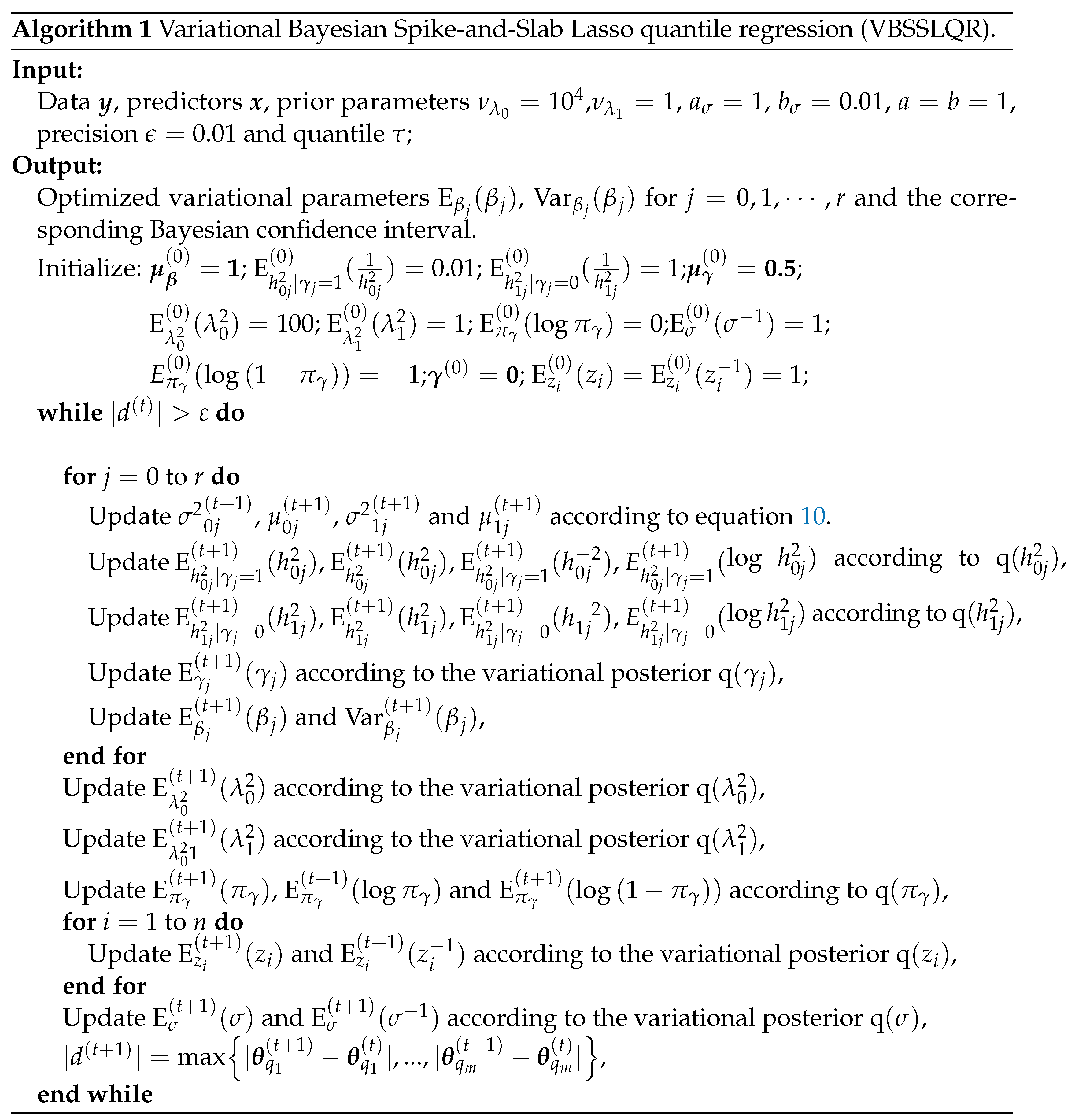
For this reason, we list the variational Bayesian Spike-and-Slab Lasso quantile regression (VBSSLQR) algorithm as shown in the following Algorithm 1:

In Algorithm 1 above, the

Ψ (\cdot)

is the digamma fuction and the expectation

E_{h_{0 j}^{2} | γ_{j} = 1}^{(t + 1)} (\log h_{0 j}^{2})

\log h_{0 j}^{2}

with respect to generalized inverse Gaussian distribution. So, we assume that

x \sim GIG (p, a, b)

, then:

\begin{matrix} E_{x} (\log x) = \frac{\frac{d K_{p} (\sqrt{a b})}{d p}}{K_{p} (\sqrt{a b})} - \frac{1}{2} \ln (\frac{a}{b}), \end{matrix}

(11)

where

K_{p} (\cdot)

represents Bessel function of the second kind. Note that there is no analytic solution or function to the differential of the Modified Bessel function. Therefore, We approcimate

E_{x} (\log x)

by the second-order Taylor expansion of

\log x

. This paper lists the expectation of some parameter functions about variational posteriors involved in algorithm Section 2.3. See Appendix B for details. Based on our proposed VBSSLQR algorithm, in the next section, we randomly generate high-dimensional data, conducting simulation research and comparing the performance of other methods.

3. Simulation Studies

In this section, we use simulated high-dimensional data with sample size

n = 200

and variable number

r = 500

, in order to study the performance of VBSSLQR and compare it with existing methods, including linear regression with the Lasso penalty (Lasso), linear regression with the adaptive Lasso penalty (ALasso), quantile regression with the Lasso penalty (QRL), quantile regression with the adaptive Lasso penalty (QRAL), Bayesian regularized quantile regression with the Lasso penalty (BLQR) and Bayesian regularized quantile regression with the adaptive Lasso penalty (BALQR). The data in the simulation studies are generated by equation (1), in which the covariate vector

x_{i}

is randomly generated from the multivariate normal distribution

N (0, Σ)

with the

{(k, l)}_{t h}

Σ

being

0 . 5^{| k - l |}

. Among these covariates, we only consider ten important explanatory variables that have significant impact on the dependent variable. We set the 1, 51, 101, 151, 201, 251, 301, 351, 401, 451 predictors to be active and their regression coefficients are -3, -2.5, -2, -1.5, -1, 1, 1.5, 2, 2.5, 3, and the rest are zero. In addition, we discuss the performance of various approachs in the case of two kinds of random errors, namely, independent and identically distributed (i.i.d.) random errors and heterogenous random errors.

3.1. Independent and Identically Distributed Random Errors Random

In this subsection, with reference to [19] and [23], we set the random errors

ε_{i}

’s in equation (1) to be independently and identically distributed and consider following five different distributions with

τ

quantile being zero for it:

The error $ε_{i} \overset{i . i . d .}{\sim} N (- μ, 1)$ with $μ$ being the $τ$ quantile of $N (0, 1)$ , for $i = 1, \dots, n$ ;
The error $ε_{i} \overset{i . i . d .}{\sim} Laplace (- μ, 1)$ with $μ$ being the $τ$ quantile of $Laplace (0, 1)$ , where $Laplace (a, b)$ denotes the Laplace distribution with location parameter a and scale parameter b;
The error $ε_{i} \overset{i . i . d .}{\sim} 0.1 N (- μ_{1}, 9) + 0.9 N (- μ_{2}, 1)$ with $μ_{1}$ and $μ_{2}$ respectively being the $τ$ quantile of $N (0, 9)$ and $N (0, 1)$ ;
The error $ε_{i} \overset{i . i . d .}{\sim} 0.1 Laplace$ $(- μ_{1}, 9) + 0.9 Laplace (- μ_{2}, 1)$ with $μ_{1}$ and $μ_{2}$ respectively being the $τ$ quantile of $Laplace (0, 9)$ and $Laplace (0, 1)$ ;
The error $ε_{i} \overset{i . i . d .}{\sim} Cauchy (- μ, 0.2)$ with $μ$ being the $τ$ quantile of $Cauchy (0, 0.2)$ , where $Cauchy (a, b)$ denotes the Cauchy distribution with location parameter a and scale parameter b;

For above any error distribution with any

τ \in (0.3, 0.5, 0.7)

, we run 500 replications for each method, and evaluate the performance by two criterion. The first criterion is the median of mean absolute deviations (MMAD), whcih quantify the general distance between the estimated conditional quantile and the true conditional quantile. Specifically, mean absolute deviation (MAD) in any replication is defined as

\frac{1}{n} \sum_{i = 1}^{n} | x_{i} β - x_{i} {\hat{β}}_{τ}) |,

where

{\hat{β}}_{τ}

is the estimate of regression coefficient

β

given

τ

. The second criterion is the mean of true positives (TP) and false positives (FP) selected by each method.

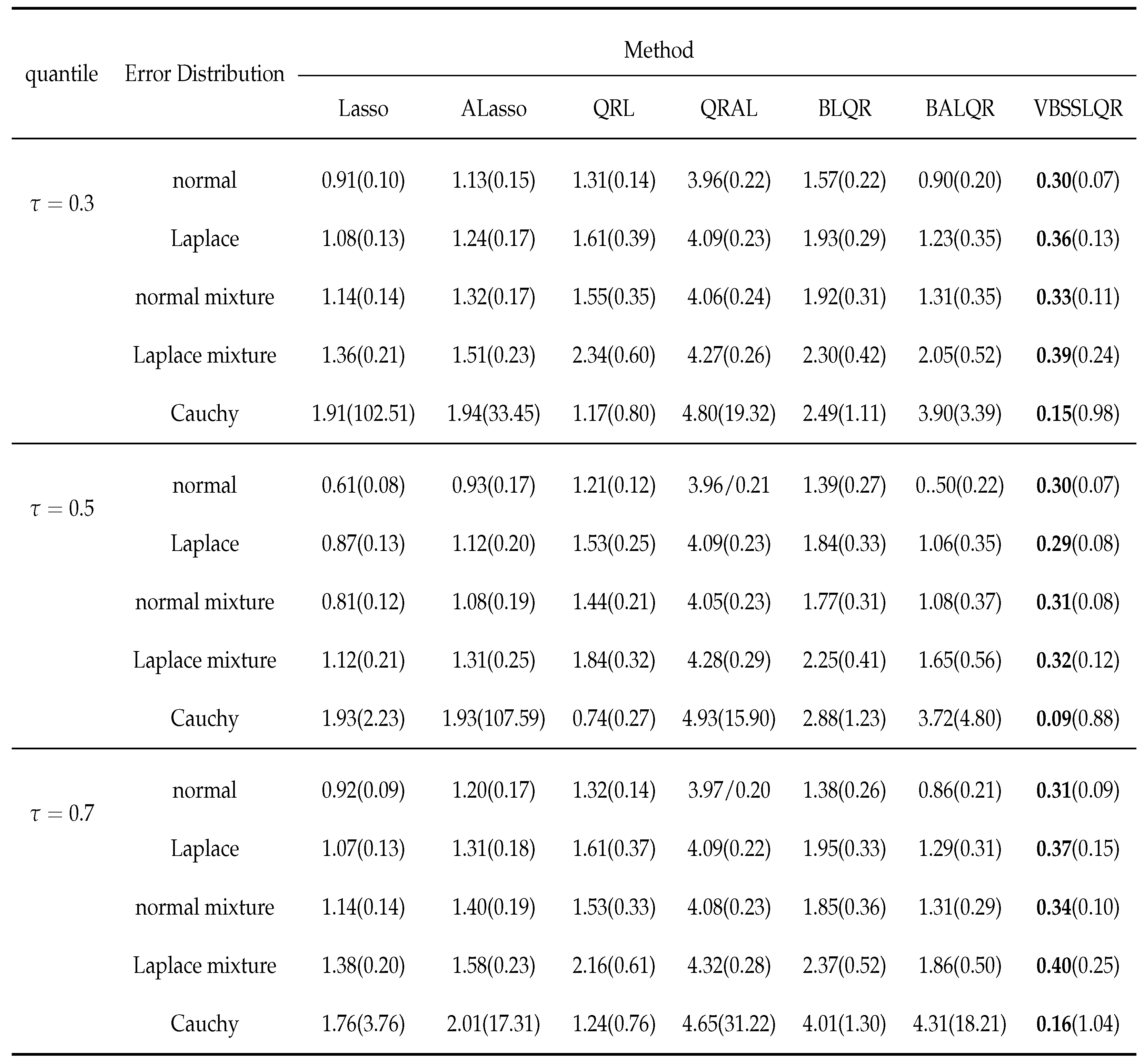
Table 1 shows the median and stndard deviation (SD) of MADs estimated by each method for simulations with homogeneous errors. It is clear that our method is either optimal (bold) in all cases, especially in quantile

τ = 0.3, 0.7

, our approach is significantly superior to the other six methods. When the error distribution is normal, Laplace and normal mixture, the MMAD of BALQR method is suboptimal. When the error distribution is Cauchy, the MMAD of the QRL approach is suboptimal, but Table 2 shows that it sacrifices the complexity of the model. When the error distribution is Laplace mixture, the MMAD of the Lasso approach is suboptimal, however it selects the over-fitting quantile regression model with about 30 FP variables, as can be seen from the Table 2. It is particularly important to note that in the case of high dimensional data, MMAD for the quantile regression model with Lasso penalty or adaptive lasso penalty is not less than MMAD for general linear models with Lasso penalty. Therefore, it is inappropriate to still use Lasso penalty or adaptive lasso in this case.

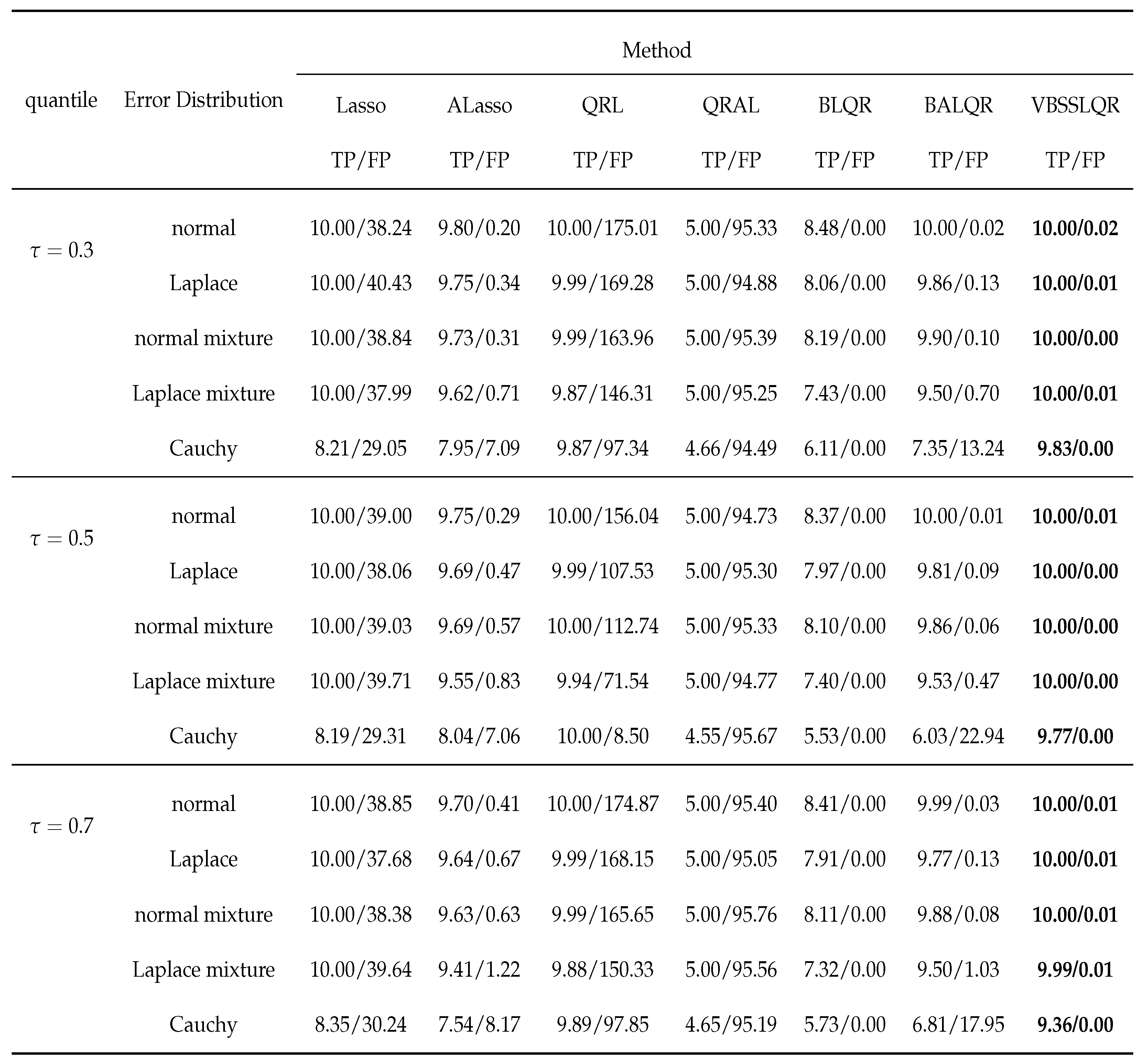
In order to show the results of variable selection more intuitively, we introduced TP (True positives) and FP (False positives) to calculate the mean of TP and FP of 500 repeated simulations respectively. The detailed results are shown in Table 2 below:

It is not difficult to conclude from the results in Table 2: Lasso method can basically select all true active variables, but it fits many false active variables, and when the random errors is Cauchy distribution, it cannot select all true active variables; ALasso approach can identify true active variables, but there are also some misjudged behaviors, especially when the random errors distribution is Cauchy distribution; Although QRL approach can identify real active variables, it still contains many false active variables, and the model it identifies has high complexity; QRAL method can not identify all true active variables, and incorrectly identifies some inactive variables; In the case of high-dimensional data, BLQR approach cannot select all the true active variables, but it also does not select the inactive variables incorrectly; The true active variable selected by BALQR method is better than that by BLQR method, but some inactive variables are selected incorrectly, especially when the random errors distribution is Cauchy distribution; Our VBSSLQR method not only has the smallest MMAD, but also can select true active variables and eliminate most false active variables. As a whole, our method is superior to the other six methods in variable selection, especially in quantile

τ = 0.3, 0.7

it is significantly better than BLQR, BALQR and QRL.

3.2. Heterogenous Random Errors

Now we consider the case of heterogenous random errors to demonstrate the performance of our method. In this subsection, the data are generated from the following model:

\begin{matrix} y_{i} = x_{i}^{⊤} β + (1 + u_{i}) ε_{i}, \end{matrix}

(12)

where

u_{i} \overset{i . i . d .}{\sim} U (0, 1)

in which

U (a, b)

represents the uniform distribution with support set

(a, b)

. The design matrix

x_{i}

is generated in the same way as above, and the regression coefficient

β

is set as before. Furthermore, in the simulation study, we combine

x_{i}

and

u_{i}

, that is,

u_{i}

is also a covariate. Finally, random error

ε_{i}

is also generated from five different distributions defined in subsection (Section 3.1).

We also studied the performance of the quantile

τ \in (0.3, 0.5, 0.7)

under different methods and simulated 500 times to calculate the MMAD and mean of TP/FP. We list the experimental results in the following two tables.

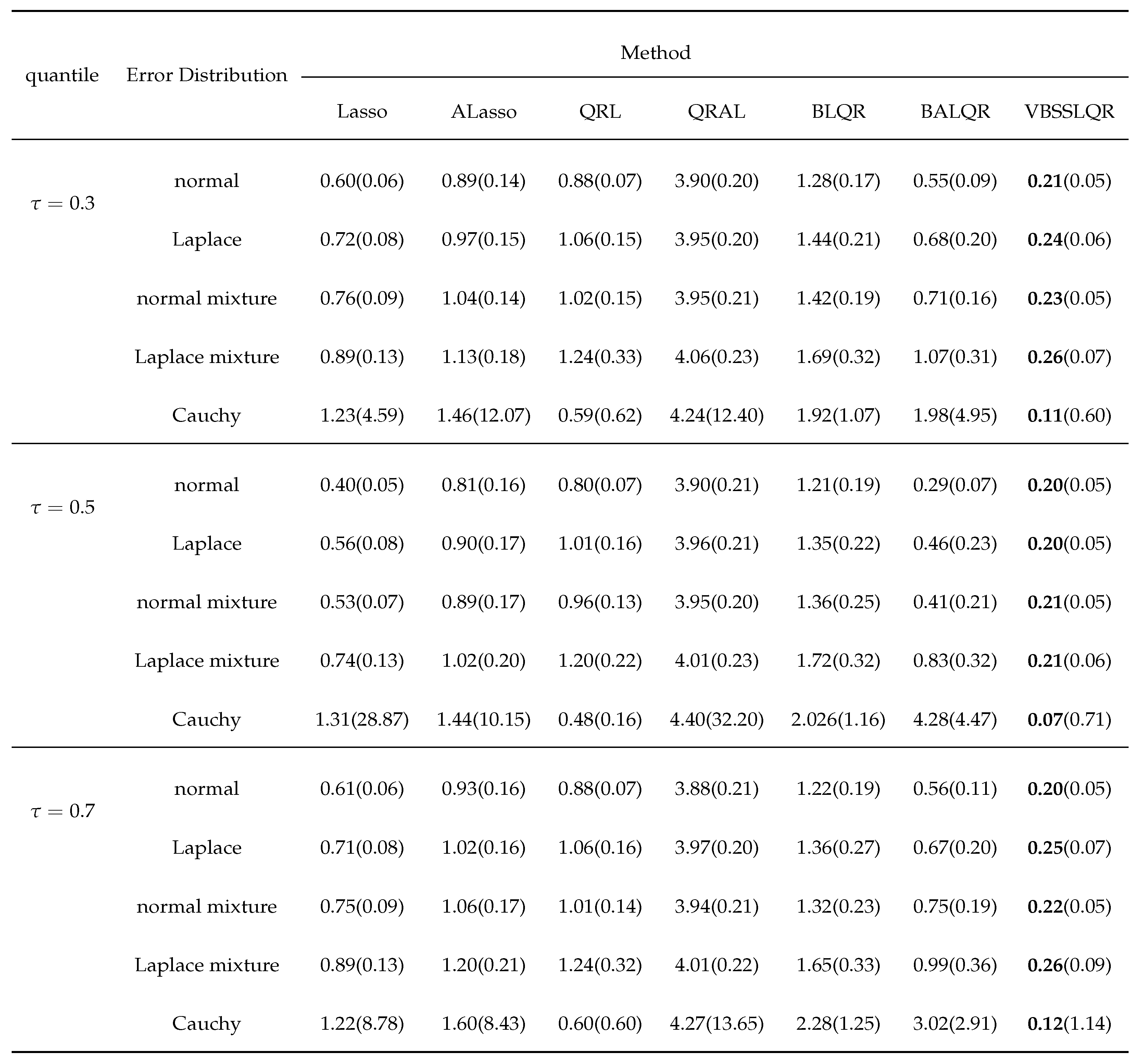
Table 3. The Median and standard deviation of 500 MADs estimated via various methods for simulations with heterogenous random errors.

In heterogenous random errors, our approach is still the best one similar to i.i.d. random errors. It is noteworthy that the VBSSLQR method is more robust than other methods, and our method has the smallest MMAD change compared to the case i.i.d. random errors. We can see that the MMAD of our method remains basically unchanged, while the MMAD of the other six methods differs even more than 0.5 compared to i.i.d. random errors in some states.

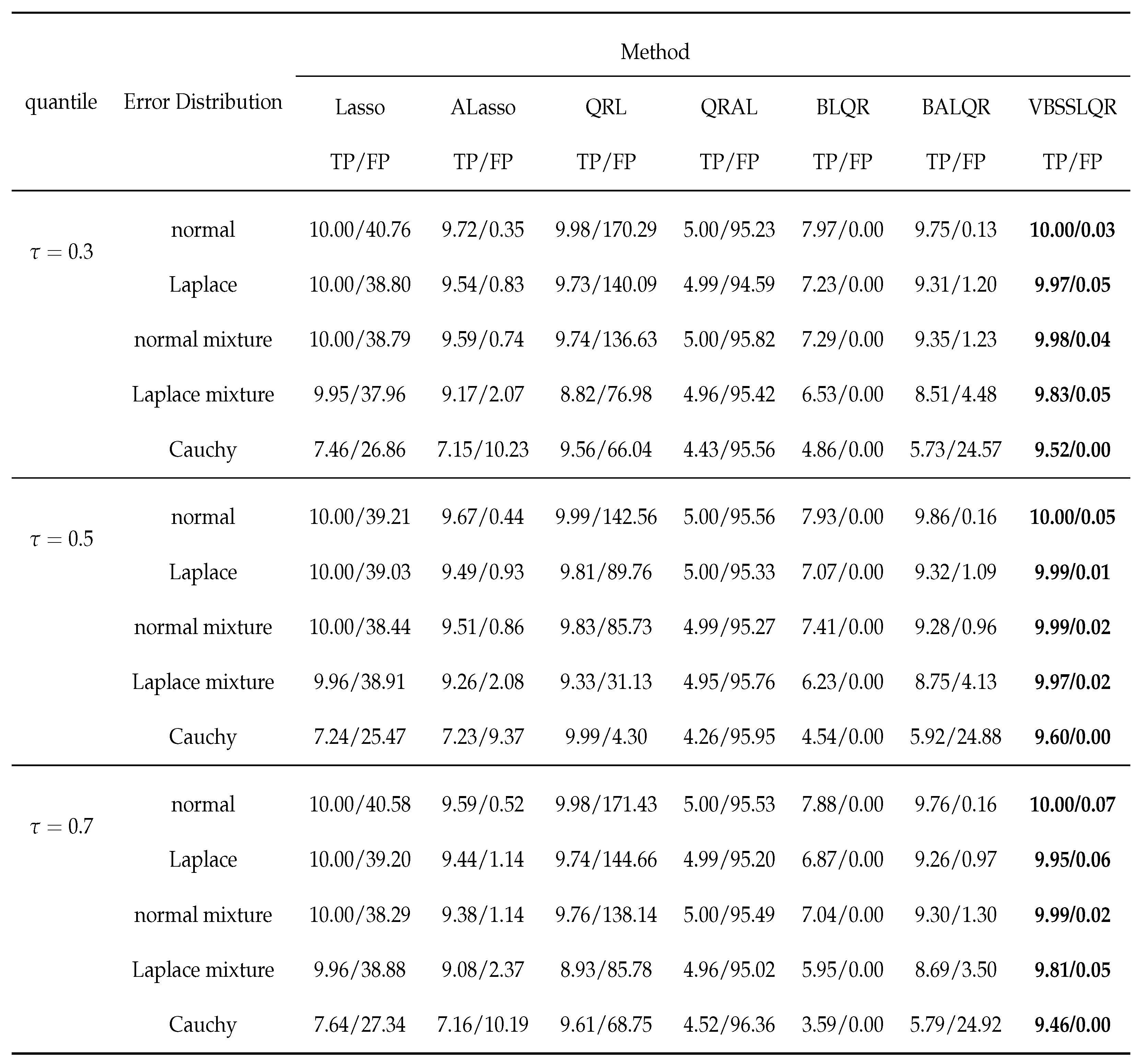
We also investigate the mean of TP and FP in heterogenous random errors under different quantiles

τ

. The results are listed in Table 4, whichs show that the effect for variable selection of heterogenous random errors is slightly lower than the effect for variable selection of i.i.d. random errors under the same sample size, but our method still provides the best selection result.

We also calculate the mean execution times of various Bayesian quantile regressions under different quantile

τ

for different distributions of random errors, and list the results in Table A1 of Appendix C, which illustrate our proposed VBSSLQR approach is a lot more efficient than BLQR and BALQR , for which we sampled MCMC 1000 times and discarded the first 500 times, and made statistical inference based on 500 samples (the experimental study shows that the algorithm has converged after 500 samples).

4. Examples

In this section, we analyze the real dataset that it contains information about crime in various cities in the United States. It is available at the University of Irvine machine learning repository (http://archive.ics.uci.edu/ml/datasets/communities+and+crime). The per capita violent crimes was calculated using population and the sum of crimevariables considered violent crimes in the United States: murder, rape, robbery, and assault. The observed individuals are communities. The dataset has 116 variables where the first four columns are response, name of community, code of county, code of community, the middle features are demographic information about each community such as population, age, race, income, and the final columns are region. According to the source: "the data combines socio-economic data from the 1990 US Census, law enforcement data from the 1990 US LEMAS survey, and crime data from the 1995 FBI UCR". This dataset has been applied to quantile regression [30]. The dataset is available at:

Our response variable of interest is the murder rate of each city (response variable

y_{i} \in [0, 1]

). We choose this variable because it is the most dangerous one among the list of violent crimes. Identifying factors correlated with murder rate will be of immense importance to law enforcement agencies and the public at large.

To adapt the data to our model, we preprocess the data as follows:

Delete columns from the data set that contain missing data.
Delete the data when the response variable $y_{i}$ equals 0 because this is not an issue of interest to us.
Transform $y_{i}$ : $y_{i}^{'} = \log \frac{y_{i}}{1 - y_{i}}$ and letting $y_{i}^{'}$ as the new response variable.
Convert some qualitative variables into quantitative variables.
Standardized covariates.

After the above data preprocessing, we get 1060 observation objects and 95 covariates in train set, and we get 122 observation objects and 95 covariates in test set. We estimate a quantile regression model between the response

y_{i}^{'}

and the 96 predictors with intercept.

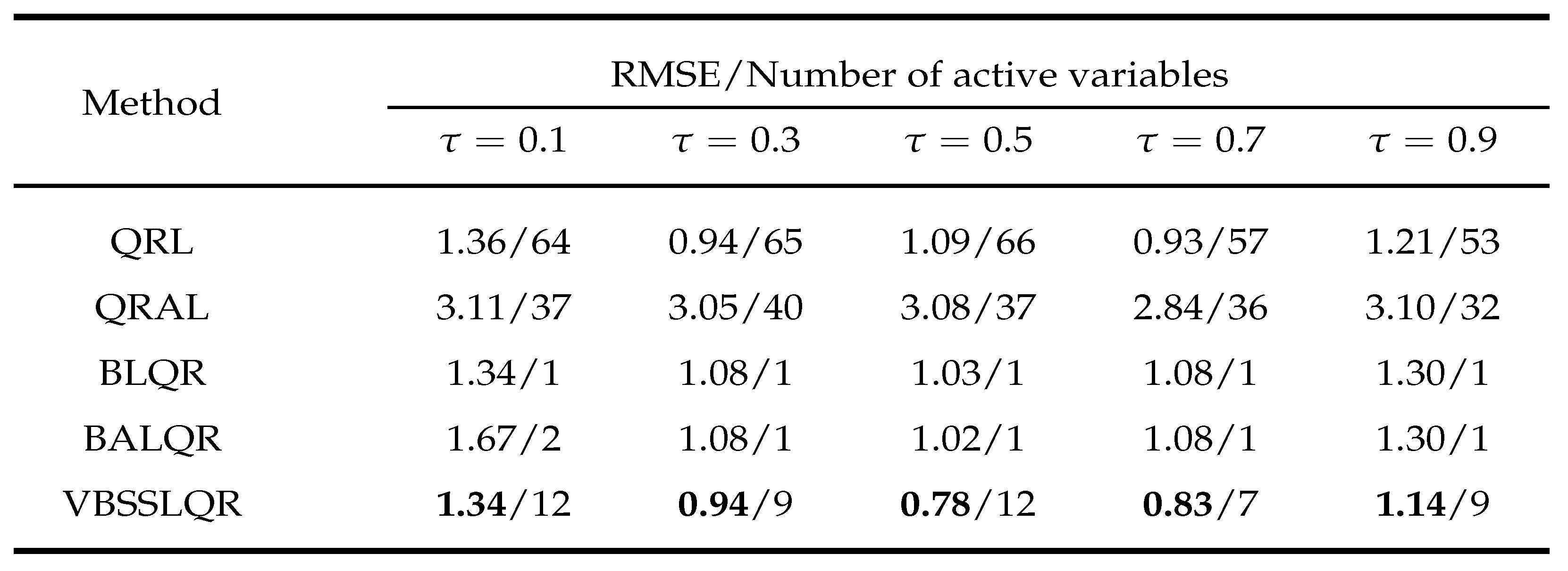
In this section, we only compare QRL, QRAL, BLQR, BALQR with our method VBSSLQR for real dataset, they are all quantile penalty regression obviously. Under different quantile

τ \in (0.1, 0.3, 0.5, 0.7, 0.9)

, we compare the performance of different approachs. We counted the Root Mean Squared Error (RMSE) of each method under each quantile

τ

and the number of selected active variables to evaluate the performance of each approach in test set, where RMSE are evaluated by

RMSE = \sqrt{\frac{1}{n} \sum_{i = 1}^{n} {(y_{i} - {\hat{y}}_{τ i})}^{2}}

with

{\hat{y}}_{τ i}

is the fitted value of response

y_{i}

under quantile

τ

. Finally, the results are listed in the Table 5 below.

To visually show the results listed in Table 4, we will use best results are bolded under each quantile

τ

. Obviously, our method performs better than other methods at all quantile and the active variables selected by our method are suitable, which means that our method is very competitive compared with other methods. BLQR and BALQR approachs can only identify the intercept, and they cannot identify the variables that really affect the response quantile. QRL and QRAL methods are prone to overfitting because they recognize too many active variables. Finally, the efficiency of our method in real data is also significantly higher than that of other approachs. So far, we believe that there are sufficient reasons to show that our method is enough competitive compared with other approachs.

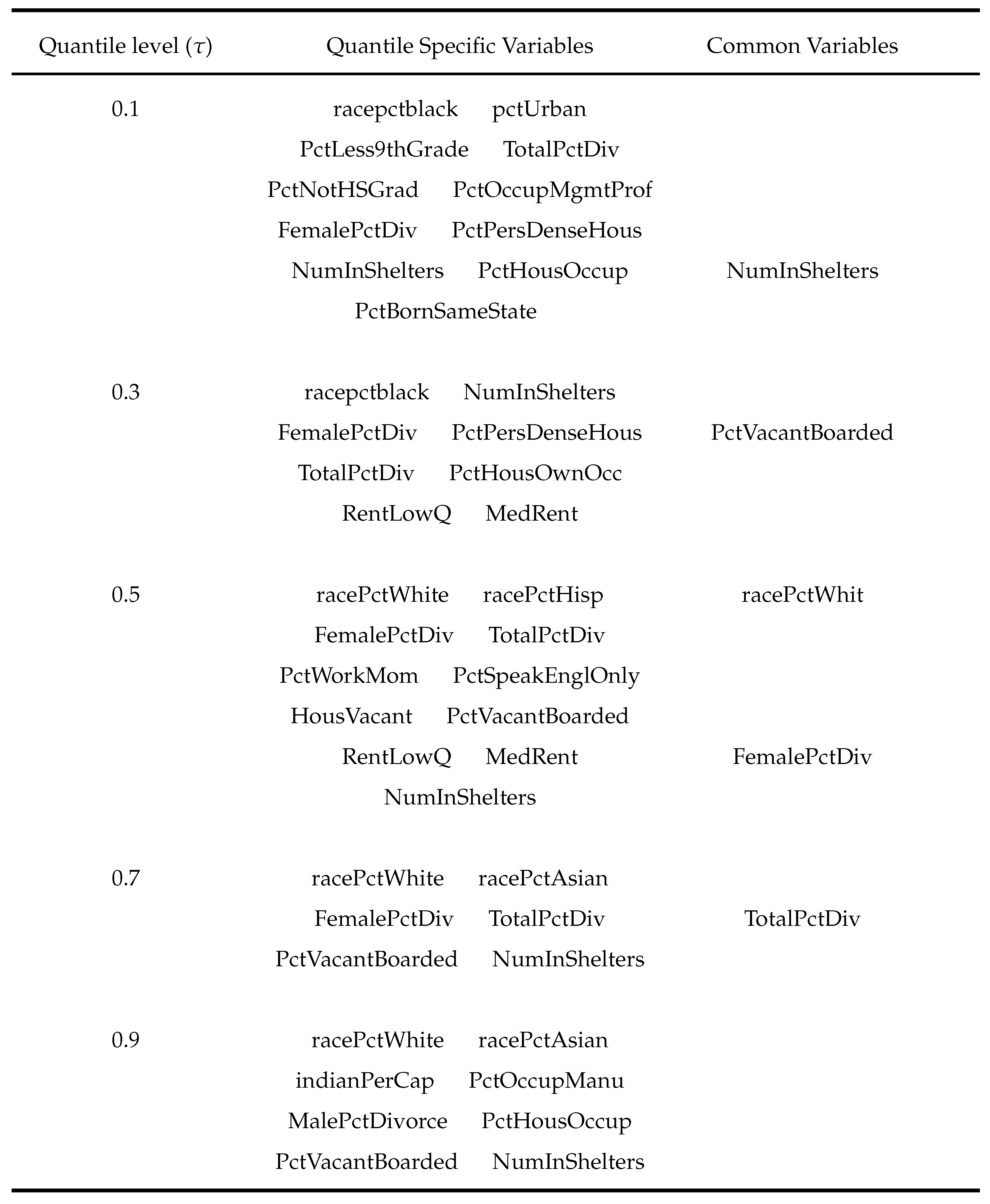
Similar to [30], we list the active variables selected under each quantile in Table 6. So, Table 6 shows the variable selection of our proposed method in real data.

In the above table, common variables represents the five variables that appear most frequently. As evident in the Table 6, our method selected only a small number of predictors at each quantile level. The common 5 variables that the model picked are:

PctVacantBoarded: percentage of households that are vacant and boarded up to prevent from vandalism.
NumInShelters: number of shelters in the community.
FemalePctDiv: percentage of females who are divorced.
TotalPctDiv: percentage of peoples who are divorced.
racePctWhite: percentage of person who are white race.

In order to get a better understanding of these five common variables we plot their correlation to the response.

Figure 1 depicts the relationship of five common variables and murder rate. Only the correlation between the NumInShelters and murder rate is not obvious, and the MalePctDivorce, RentLowQ, racePctWhite, PctVacantBoarded significantly affecting murder rate. The racePctWhite and murder rate are negatively correlated, while FemalePctDiv, TotalPctDiv, PctVacantBoarded and murder rate are positively correlated. The result was in accord with the practical situation and it can be seen that our results are basically consistent with that of [30], besides our method can more comprehensively select important variables under the same quantile. Therefore, percentage of females who are divorced, percentage of persons who are divorced, percentage of households that are vacant and boarded up to prevent from vandalism and percentage of person who are white race affect the murder rate.

5. Conclusions

In this paper, we propose variational Bayesian Spike-and-Slab Lasso quantile regression variable selection and estimation. This method applies Spike-and-Slab Lasso prior to each regression coefficient

β

, thus punishing the regression coefficient

β

. The spike prior distribution we choose is a small variance Laplace distribution, while the Slab prior distribution is a large variance Laplace distribution [26]. It is precisely because it punishes each regression coefficient

β

, giving it a powerful variable selection function, but it also brings a problem of low efficiency, especially when introducing Spike-and-Slab prior into quantile regression (Note, the algorithm efficiency of quantile regression is inherently lower than that of general regression approachs). In order to solve the problem of inefficiency (influenced by both quantile regression and Spike-and-Slab Lasso prior) and make the algorithm feasible, we introduce the variational Bayesian method to approximate the posterior distribution of each parameter. Simulation studies and real data analyses show that variational Bayesian Spike-and-Slab Lasso quantile regression performs well and has strong competitiveness compared with other approachs (Bayesian method or non-Bayesian method, quantile regression or non-quantile regression), especially in the case of high-dimensional data.

Author Contributions

Conceptualization, D.D. and A.T.; methodology, D.D. and A.T. ; software, D.D. and J.Y.; validation, D.D., J.Y. and A.T.; formal analysis, D.D. and A.T; investigation, D.D., J.Y. and A.T.; Preparation of the original work draft, A.T. and D.D.; visualization, D.D. and J.Y.; supervision, funding acquisition, D.D., A.T. and J.Y.. All authors have read and agreed to the published version of the manuscript.

Funding

This work was supported by the National Natural Science Foundation of China (No. 11961079) and Yunnan Univeristy Multidisciplinary Team Construction Projects in 2023.

Institutional Review Board Statement

Not applicable.

Informed Consent Statement

Not applicable.

Data Availability Statement

The research data is available on the website http://archive.ics.uci.edu/ml/datasets/communities+and+crime

Conflicts of Interest

The authors declare no conflict of interest.

Appendix A. Deduction

Based on the mean-field variational formula (9), from the joint density (8), it is direct to induce the following variational distributions.

\begin{matrix} q (β_{j}, γ_{j}) \propto & \exp \{E_{- β_{j}, γ_{j}} [\sum_{i =}^{n} \log N (y_{i} | x_{i}^{⊤} β + k_{1} z_{i}, k_{2} σ z_{i}) + γ_{j} \log N (β_{j} | 0, h_{0 j}^{2}) \\ + (1 - γ_{j}) \log N (β_{j} | 0, h_{0 j}^{2}) + \log B (γ_{j} | 1, π_{γ})]\} \\ \propto & \exp \{- \frac{1}{2 k_{2}} E_{σ} (σ^{- 1}) [\sum_{i = 1}^{n} E_{z_{i}} (z_{i}^{- 1}) x_{i j}^{2} β_{j}^{2} + 2 \sum_{i = 1}^{n} x_{i j} (E_{z_{i}} (z_{i}^{- 1}) \\ (y_{i} - x_{i, (- j)}^{⊤} μ_{β_{(- j)}}) - k_{1}) β_{j}] - \frac{γ_{j}}{2} E_{h_{0 j}^{2}} (\log 2 π h_{0 j}^{2}) - \frac{γ_{j}}{2} E_{h_{0 j}^{2}} (\frac{1}{h_{0 j}^{2}}) β_{j}^{2} \\ - \frac{(1 - γ_{j})}{2} E_{h_{1 j}^{2}} (\log 2 π h_{1 j}^{2}) - \frac{(1 - γ_{j})}{2} E_{h_{0 j}^{2}} (\frac{1}{h_{1 j}^{2}}) β_{j}^{2} + γ_{j} E_{π_{γ}} (\log π_{γ}) \\ + (1 - γ_{j}) E_{π_{γ}} (\log (1 - π_{γ}))\} \\ \propto & \exp \{[- \frac{1}{2 k_{2}} E_{σ} (σ^{- 1}) \sum_{i = 1}^{n} E_{z_{i}} (z_{i}^{- 1}) x_{i j}^{2} - \frac{γ_{j}}{2} E_{h_{0 j}^{2}} (\frac{1}{h_{0 j}^{2}}) - \frac{(1 - γ_{j})}{2} E_{h_{0 j}^{2}} (\frac{1}{h_{1 j}^{2}})] β_{j}^{2} \\ - \frac{1}{k_{2}} \sum_{i = 1}^{n} x_{i j} (E_{z_{i}} (z_{i}^{- 1}) (y_{i} - x_{i, (- j)}^{⊤} μ_{β_{(- j)}}) - k_{1}) β_{j} + γ_{j} E_{π_{γ}} (\log π_{γ}) \\ + (1 - γ_{j}) E_{π_{γ}} (\log (1 - π_{γ})) - \frac{γ_{j}}{2} E_{h_{0 j}^{2}} (\log 2 π h_{0 j}^{2}) - \frac{(1 - γ_{j})}{2} E_{h_{1 j}^{2}} (\log 2 π h_{1 j}^{2})\}, \end{matrix}

where

μ_{β_{(- j)}} = E_{β_{(- j)}} (β_{(- j)})

. therefore, given

γ_{j} = k

, for k = 0,1, then

\begin{matrix} q (β_{j} | γ_{j} = k) \propto & \exp \{E_{- β_{j} | γ_{j} = k} [\sum_{i =}^{n} \log N (y_{i} | x_{i}^{⊤} β + k_{1} z_{i}, k_{2} σ z_{i}) + k \log N (β_{j} | 0, h_{0 j}^{2}) \\ + (1 - k) \log N (β_{j} | 0, h_{0 j}^{2})]\}, \end{matrix}

γ_{j} = 0

then

\begin{matrix} q (β_{j} | γ_{j} = 0) \propto & \exp \{[- \frac{1}{2 k_{2}} E_{σ} (σ^{- 1}) \sum_{i = 1}^{n} E_{z_{i}} (z_{i}^{- 1}) x_{i j}^{2} - \frac{1}{2} E_{h_{1 j}^{2} | γ_{j} = 0} (\frac{1}{h_{1 j}^{2}})] β_{j}^{2} \\ - \frac{1}{k_{2}} \sum_{i = 1}^{n} x_{i j} (E_{z_{i}} (z_{i}^{- 1}) (y_{i} - x_{i, (- j)}^{⊤} μ_{β_{(- j)}}) - k_{1}) β_{j}\}, \\ β_{j} | γ_{j} = 0 \overset{i . i . d .}{\sim} & N (μ_{1 j}, σ_{1 j}^{2}), \end{matrix}

γ_{j} = 1

then

\begin{matrix} q (β_{j} | γ_{j} = 1) \propto & \exp \{[- \frac{1}{2 k_{2}} E_{σ} (σ^{- 1}) \sum_{i = 1}^{n} E_{z_{i}} (z_{i}^{- 1}) x_{i j}^{2} - \frac{1}{2} E_{h_{0 j}^{2} | γ_{j} = 1} (\frac{1}{h_{0 j}^{2}})] β_{j}^{2} \\ - \frac{1}{k_{2}} \sum_{i = 1}^{n} x_{i j} (E_{z_{i}} (z_{i}^{- 1}) (y_{i} - x_{i, (- j)}^{⊤} μ_{β_{(- j)}}) - k_{1}) β_{j}\}, \\ β_{j} | γ_{j} = 1 \overset{i . i . d .}{\sim} & N (μ_{0 j}, σ_{0 j}^{2}), \end{matrix}

therefore

β_{j} \overset{i . i . d .}{\sim} \sum_{k = 0}^{1} p (γ_{j} = k) N (μ_{k j}, σ_{k j}^{2}), for j = 0, 1, \dots, r

, where

\begin{matrix} μ_{k j} = σ_{k j}^{2} \frac{E_{σ} (σ^{- 1})}{k_{2}} \sum_{i = 1}^{n} [E_{z_{i}} (z_{i}^{- 1}) (y_{i} - x_{i, (- j)}^{⊤} μ_{β_{(- j)}}) - k_{1}] x_{i j}, \\ σ_{k j}^{2} = {[E_{h_{k j}^{2} | γ_{j} = 1 - k} (h_{k j}^{- 2}) + \frac{E_{σ} (σ^{- 1})}{k_{2}} \sum_{i = 1}^{n} x_{i j}^{2} E_{z_{i}} (z_{i}^{- 1})]}^{- 1}, \end{matrix}

for

k = 1

and 2. similarly, if

γ_{j} = 1

then

\begin{matrix} q (h_{0 j}^{2} | γ_{j} = 1) \propto & \exp \{E_{- h_{0 j}^{2} | γ_{j} = 1} [\log N (β_{j} | 0, h_{0 j}^{2}) + \log Exp (h_{0 j}^{2} | \frac{λ_{0}^{2}}{2})]\} \\ \propto & {(h_{0 j}^{2})}^{- \frac{1}{2}} \exp \{- \frac{E_{β_{j} | γ_{j} = 1} (β_{j}^{2})}{2 h_{0 j}^{2}} - \frac{E_{λ_{0}^{2}} (λ_{0}^{2})}{2} h_{0 j}^{2}\} \\ = & {(h_{0 j}^{2})}^{- \frac{1}{2}} \exp \{- \frac{1}{2} [\frac{μ_{0 j}^{2} + σ_{0 j}^{2}}{h_{0 j}^{2}} + E_{λ_{0}^{2}} (λ_{0}^{2}) h_{0 j}^{2}]\}, \\ h_{0 j}^{2} | γ_{j} = 1 \overset{i . i . d .}{\sim} & GIG (\frac{1}{2}, E_{λ_{0}^{2}} (λ_{0}^{2}), μ_{0 j}^{2} + σ_{0 j}^{2}), \end{matrix}

γ_{j} = 0

then

\begin{matrix} q (h_{0 j}^{2} | γ_{j} = 0) \propto & {(h_{0 j}^{2})}^{- \frac{1}{2}} \exp \{- \frac{1}{2} E_{λ_{0}^{2}} (λ_{0}^{2}) h_{0 j}^{2}\}, \\ h_{0 j}^{2} | γ_{j} = 0 \overset{i . i . d .}{\sim} & Exp (\frac{1}{2} E_{λ_{0}^{2}} (λ_{0}^{2})), \end{matrix}

therefore

\begin{matrix} q (h_{0 j}^{2}) = p (γ_{j} = 1) GIG (\frac{1}{2}, E_{λ_{0}^{2}} (λ_{0}^{2}), σ_{0 j}^{2} + μ_{0 j}^{2}) + p (γ_{j} = 0) Exp (\frac{1}{2} E_{λ_{0}^{2}} (λ_{0}^{2})) . \end{matrix}

similarly,

\begin{matrix} q (h_{1 j}^{2}) = p (γ_{j} = 0) GIG (\frac{1}{2}, E_{λ_{1}^{2}} (λ_{1}^{2}), σ_{1 j}^{2} + μ_{1 j}^{2}) + p (γ_{j} = 1) Exp (\frac{1}{2} E_{λ_{1}^{2}} (λ_{1}^{2})), \end{matrix}

where

μ_{k j}

and

σ_{k j}^{2}

are the same as above, for

k = 1

and 0, from

q (β_{j}, γ_{j})

then

\begin{matrix} q (β_{j}, γ_{j} = 1) = & C \exp \{- \frac{1}{2} σ_{0 j}^{- 2} β_{j}^{2} + \frac{μ_{0 j}}{σ_{0 j}^{2}} β_{j} + E_{π_{γ}} (\log π_{γ}) - \frac{1}{2} E_{h_{0 j}^{2} | γ_{j} = 1} (\log h_{0 j}^{2})\}, \end{matrix}

integral out

β_{j}

obtain

\begin{matrix} p (γ_{j} = 1) & = \int q (β_{j}, γ_{j} = 1) d β_{j} \\ = C \sqrt{σ_{0 j}^{2}} \exp \{μ_{0 j}^{2} {(2 σ_{0 j}^{2})}^{- 1} + E_{π_{γ}} (\log π_{γ}) - \frac{1}{2} E_{h_{0 j}^{2} | γ_{j} = 1} (\log h_{0 j}^{2})\} . \end{matrix}

similarly,

\begin{matrix} p (γ_{j} = 0) & = \int q (β_{j}, γ_{j} = 0) d β_{j} \\ = C \sqrt{σ_{1 j}^{2}} \exp \{μ_{1 j}^{2} {(2 σ_{1 j}^{2})}^{- 1} + E_{π_{γ}} (\log (1 - π_{γ})) - \frac{1}{2} E_{h_{1 j}^{2} | γ_{j} = 0} (\log h_{1 j}^{2})\} . \end{matrix}

letting

\begin{matrix} ζ_{j} = & \log p (γ_{j} = 0) - \log p (γ_{j} = 1) \\ = & E_{π_{γ}} (\log (1 - π_{γ})) - E_{π_{γ}} (\log π_{γ}) + \frac{1}{2} E_{h_{0 j}^{2} | γ_{j} = 1} (\log h_{0 j}^{2}) \\ - & \frac{1}{2} E_{h_{1 j}^{2} | γ_{j} = 0} (\log h_{1 j}^{2}) + \frac{1}{2} (\log σ_{1 j}^{2} - \log σ_{0 j}^{2}) + \frac{1}{2} (μ_{1 j}^{2} {(σ_{1 j}^{2})}^{- 1} - μ_{0 j}^{2} {(σ_{0 j}^{2})}^{- 1}), \end{matrix}

then

\begin{matrix} p (γ_{j} = 1) = \frac{1}{1 + e^{ζ_{i}}}, p (γ_{j} = 0) = \frac{e^{ζ_{i}}}{1 + e^{ζ_{i}}}, \end{matrix}

therefore

γ_{j} \overset{i . i . d .}{\sim} B (1, {(1 + e^{ζ_{i}})}^{- 1})

, for

j = 0, 1, \dots, r

, where

μ_{k j}

and

σ_{k j}^{2}

are the same as above, for

k = 1

and 2.

\begin{matrix} q (λ_{0}^{2}) \propto & \exp \{E_{- λ_{0}^{2}} [\sum_{j = 0}^{r} \log Exp (h_{0 j}^{2} | \frac{λ_{0}^{2}}{2}) + \log π (λ_{0}^{2})]\} \\ \propto & {(λ_{0}^{2})}^{ν_{λ_{0}} + r + 1 - 1} \exp \{- \frac{\sum_{j = 0}^{r} E_{h_{0 j}^{2}} (h_{0 j}^{2})}{2} λ_{0}^{2} - λ_{0}^{2}\} \\ λ_{0}^{2} \sim & Ga (ν_{λ_{0}} + r + 1, \frac{\sum_{j = 0}^{r} E_{h_{0 j}^{2}} (h_{0 j}^{2})}{2} + 1), \end{matrix}

similarly,

\begin{matrix} λ_{1}^{2} \sim & Ga (ν_{λ_{1}} + r + 1, \frac{\sum_{j = 0}^{r} E_{h_{1 j}^{2}} (h_{1 j}^{2})}{2} + 1), \end{matrix}

where

ν_{λ_{0}}

and

ν_{λ_{1}}

are hyperparameters.

\begin{matrix} q (π_{γ}) \propto & \exp \{E_{- π_{γ}} [\sum_{j = 0}^{r} \log B (γ_{j} | 1, π_{γ}) + \log π (π_{γ})]\} \\ = & \exp \{\sum_{j = 0}^{r} E_{γ_{j}} (γ_{j}) \log π_{γ} + (r + 1 - \sum_{j = 0}^{r} E_{γ_{j}} (γ_{j})) \log (1 - π_{γ}) \\ + (a - 1) \log π_{γ} + (b - 1) \log (1 - π_{γ})} \\ = & {(π_{γ})}^{a - 1 + \sum_{j = 0}^{r} E_{γ_{j}} (γ_{j})} {(1 - π_{γ})}^{r + b + 1 - 1 - \sum_{j = 0}^{r} E_{γ_{j}} (γ_{j})}, \end{matrix}

therefore

π_{γ} \sim Be (a + \sum_{j = 0}^{r} E_{γ_{j}} (γ_{j}), r + b + 1 - \sum_{j = 0}^{r} E_{γ_{j}} (γ_{j}))

where a, b are hyperparameters.

\begin{matrix} q (z_{i}) \propto & \exp \{E_{- z_{i}} [\log N (y_{i} | x_{i}^{⊤} β + k_{1} z_{i}, k_{2} σ z_{i}) + \log E (z_{i} | σ^{- 1})]\} \\ \propto & z_{i}^{\frac{1}{2} - 1} \exp \{- \frac{1}{2} [\frac{E_{σ} (σ^{- 1})}{k_{2}} ((k_{1}^{2} + 2 k_{2}) z_{i} + \frac{{(y_{i} - x_{i}^{⊤} μ_{β})}^{2} + x_{i}^{⊤} Σ_{β} x_{i}}{z_{i}})]\}, \end{matrix}

therefore

z_{i} \overset{i . i . d .}{\sim} GIG (\frac{1}{2}, a_{z_{i}}, b_{z_{i}})

, for

i = 1, \dots, n

, where

\begin{matrix} a_{z_{i}} = \frac{E_{σ} (σ^{- 1})}{k_{2}} (k_{1}^{2} + 2 k_{2}), b_{z_{i}} = \frac{E_{σ} (σ^{- 1})}{k_{2}} [{(y_{i} - x_{i}^{⊤} μ_{β})}^{2} + x_{i}^{⊤} Σ_{β} x_{i}], \end{matrix}

with

k_{1}

and

k_{2}

being constants and

Σ_{β}

is a

(p + 1) \times (p + 1)

diagonal matrix with

j_{t h}

entry being

Var (β_{j})

\begin{matrix} q (σ) \propto & \exp \{E_{- σ} [\sum_{i = 1}^{n} \log N (y_{i} | x_{i}^{⊤} β + k_{1} z_{i}, k_{2} σ z_{i}) + \log E (z_{i} | σ^{- 1}) + \log π (σ)]\} \\ \propto & {(\frac{1}{σ})}^{\frac{n}{2} + n + a_{σ} - 1} \exp \{- \frac{1}{2 k_{2}} [k_{1}^{2} E_{z_{i}} (z_{i}) + E_{z_{i}} (z_{i}^{- 1}) ({(y_{i} - x_{i}^{⊤} μ_{β})}^{2} + x_{i}^{⊤} Σ_{β} x_{i}) \\ - 2 k_{1} (y_{i} - x_{i}^{⊤} μ_{β})] σ^{- 1} - \sum_{i = 1}^{n} E_{z_{i}} (z_{i}) σ^{- 1} - b_{σ} σ^{- 1}\}, \end{matrix}

therefore

σ \sim IG (\frac{3}{2} n + a_{σ}, c_{σ})

, where

a_{σ}

b_{σ}

are hyperparameters and

\begin{matrix} c_{σ} = & \frac{1}{2 k_{2}} \sum_{i = 1}^{n} {k_{1}^{2} E_{z_{i}} (z_{i}) + E_{z_{i}} (z_{i}^{- 1}) [{(y_{i} - x_{i}^{⊤} μ_{β})}^{2} + x_{i}^{⊤} Σ_{β} x_{i}] \\ - 2 k_{1} (y_{i} - x_{i}^{⊤} μ_{β})} + \sum_{i = 1}^{n} E_{z_{i}} (z_{i}) + b_{σ} . \end{matrix}

Appendix B. Expectation

The expectation of some parameter functions about variational posteriors:

Since

β_{j} \overset{i . i . d .}{\sim} \sum_{k = 0}^{1} p (γ_{j} = k) N (μ_{k j}, σ_{k j}^{2})

, therefore

\begin{matrix} E_{β_{j}} (β_{j}) = \sum_{k = 0}^{1} p (γ_{j} = k) E_{β_{j} | γ_{j} = k} (β_{j}) = \sum_{k = 0}^{1} p (γ_{j} = k) μ_{k j}, \end{matrix}

\begin{matrix} {Var}_{β_{j}} (β_{j}) = p (γ_{j} = 1) σ_{0 j}^{2} + p (γ_{j} = 0) σ_{1 j}^{2} + p (γ_{j} = 1) p (γ_{j} = 0) {(μ_{0 j} - μ_{1 j})}^{2}, \end{matrix}

\begin{matrix} E_{β_{j} | γ_{j} = k} (β_{j}^{2}) = μ_{k j}^{2} + σ_{k j}^{2}, k = 0, 1 . \end{matrix}

Since

h_{0 j}^{2} \overset{i . i . d .}{\sim} p (γ_{j} = 1) GIG (\frac{1}{2}, E_{λ_{0}^{2}} (λ_{0}^{2}), σ_{0 j}^{2} + μ_{0 j}^{2}) + p (γ_{j} = 0) Exp (\frac{1}{2} E_{λ_{0}^{2}} (λ_{0}^{2}))

, therefore

\begin{matrix} E_{h_{0 j}^{2}} (\frac{1}{h_{0 j}^{2}}) = \sum_{k = 0}^{1} p (γ_{j} = k) E_{h_{0 j}^{2} | γ_{j} = k} (\frac{1}{h_{0 j}^{2}}), \end{matrix}

where

E_{h_{0 j}^{2} | γ_{j} = 1} (\frac{1}{h_{0 j}^{2}}) = \sqrt{E_{λ_{0}^{2}} (λ_{0}^{2}) {(E_{β_{j} | γ_{j} = 1} (β_{j}^{2}))}^{- 1}}

and

E_{h_{0 j}^{2} | γ_{j} = 0} (\frac{1}{h_{0 j}^{2}}) = 2 {[E_{λ_{0}^{2}} (λ_{0}^{2})]}^{- 1}

\begin{matrix} E_{h_{0 j}^{2} | γ_{j} = 1} (h_{0 j}^{2}) = \sqrt{E_{β_{j} | γ_{j} = 1} (β_{j}^{2}) {(E_{λ_{0}^{2}} (λ_{0}^{2}))}^{- 1}} + {(E_{λ_{0}^{2}} (λ_{0}^{2}))}^{- 1} . \end{matrix}

Since

h_{1 j}^{2} \overset{i . i . d .}{\sim} p (γ_{j} = 0) GIG (\frac{1}{2}, E_{λ_{1}^{2}} (λ_{1}^{2}), σ_{1 j}^{2} + μ_{1 j}^{2}) + p (γ_{j} = 1) Exp (\frac{1}{2} E_{λ_{1}^{2}} (λ_{1}^{2}))

, therefore

\begin{matrix} E_{h_{1 j}^{2}} (\frac{1}{h_{1 j}^{2}}) = \sum_{k = 0}^{1} p (γ_{j} = k) E_{h_{1 j}^{2} | γ_{j} = k} (\frac{1}{h_{1 j}^{2}}), \end{matrix}

where

E_{h_{1 j}^{2} | γ_{j} = 1} (\frac{1}{h_{1 j}^{2}}) = 2 {[E_{λ_{1}^{2}} (λ_{1}^{2})]}^{- 1}

and

E_{h_{1 j}^{2} | γ_{j} = 0} (\frac{1}{h_{1 j}^{2}}) = \sqrt{E_{λ_{1}^{2}} (λ_{1}^{2}) {(E_{β_{j} | γ_{j} = 0} (β_{j}^{2}))}^{- 1}}

\begin{matrix} E_{h_{1 j}^{2} | γ_{j} = 0} (h_{1 j}^{2}) = \sqrt{E_{β_{j} | γ_{j} = 0} (β_{j}^{2}) {(E_{λ_{1}^{2}} (λ_{1}^{2}))}^{- 1}} + {(E_{λ_{1}^{2}} (λ_{1}^{2}))}^{- 1} . \end{matrix}

Since

σ \sim IG (\frac{3}{2} n + a_{σ}, c_{σ})

, therefore

\begin{matrix} E_{σ} (σ^{- 1}) = (\frac{3}{2} n + a_{σ}) \frac{1}{c_{σ}}, E_{σ} (σ) = {(\frac{3}{2} n + a_{σ} - 1)}^{- 1} c_{σ}, \end{matrix}

Since

z_{i} \overset{i . i . d .}{\sim} GIG (\frac{1}{2}, a_{z_{i}}, b_{z_{i}})

, therefore

\begin{matrix} E_{z_{i}} (z_{i}^{- 1}) = \sqrt{a_{z_{i}} {(b_{z_{i}})}^{- 1}}, E_{z_{i}} (z_{i}) = \sqrt{b_{z_{i}} {(a_{z_{i}})}^{- 1}} + {(a_{z_{i}})}^{- 1} . \end{matrix}

Since

λ_{k}^{2} \sim Ga (ν_{λ_{k}} + r + 1, \frac{\sum_{j = 0}^{r} E_{h_{k j}^{2}} (h_{k j}^{2})}{2} + 1)

, for

k = 0

and 1, therefore

\begin{matrix} E_{λ_{k}^{2}} (λ_{k}^{2}) = (r + 1 + ν_{λ_{k}}) {(1 + \frac{1}{2} \sum_{j = 0}^{r} E_{h_{k j}^{2}} (h_{k j}^{2}))}^{- 1} . \end{matrix}

Since

π_{γ} \sim Be (a + \sum_{j = 0}^{r} E_{γ_{j}} (γ_{j}), r + b + 1 - \sum_{j = 0}^{r} E_{γ_{j}} (γ_{j}))

, therefore

\begin{matrix} E_{π_{γ}} (\log π_{γ}) = Ψ (a + \sum_{j = 0}^{r} E_{γ_{j}} (γ_{j})) - Ψ (a + b + r + 1), \end{matrix}

\begin{matrix} E_{π_{γ}} (\log (1 - π_{γ})) = Ψ (r + b + 1 - \sum_{j = 0}^{r} E_{γ_{j}} (γ_{j})) - Ψ (a + b + r + 1), \end{matrix}

\begin{matrix} E_{π_{γ}} (π_{γ}) = (a + \sum_{j = 0}^{r} E_{γ_{j}} (γ_{j})) {(a + r + b + 1)}^{- 1} . \end{matrix}

Since

γ_{j} \overset{i . i . d .}{\sim} B (1, {(1 + e^{ζ_{i}})}^{- 1})

, therefore

\begin{matrix} E_{γ_{j}} (γ_{j}) = p (γ_{j} = 1) = {(1 + e^{ζ_{i}})}^{- 1} . \end{matrix}

Appendix C. Efficiency comparison between Bayesian quantile regression

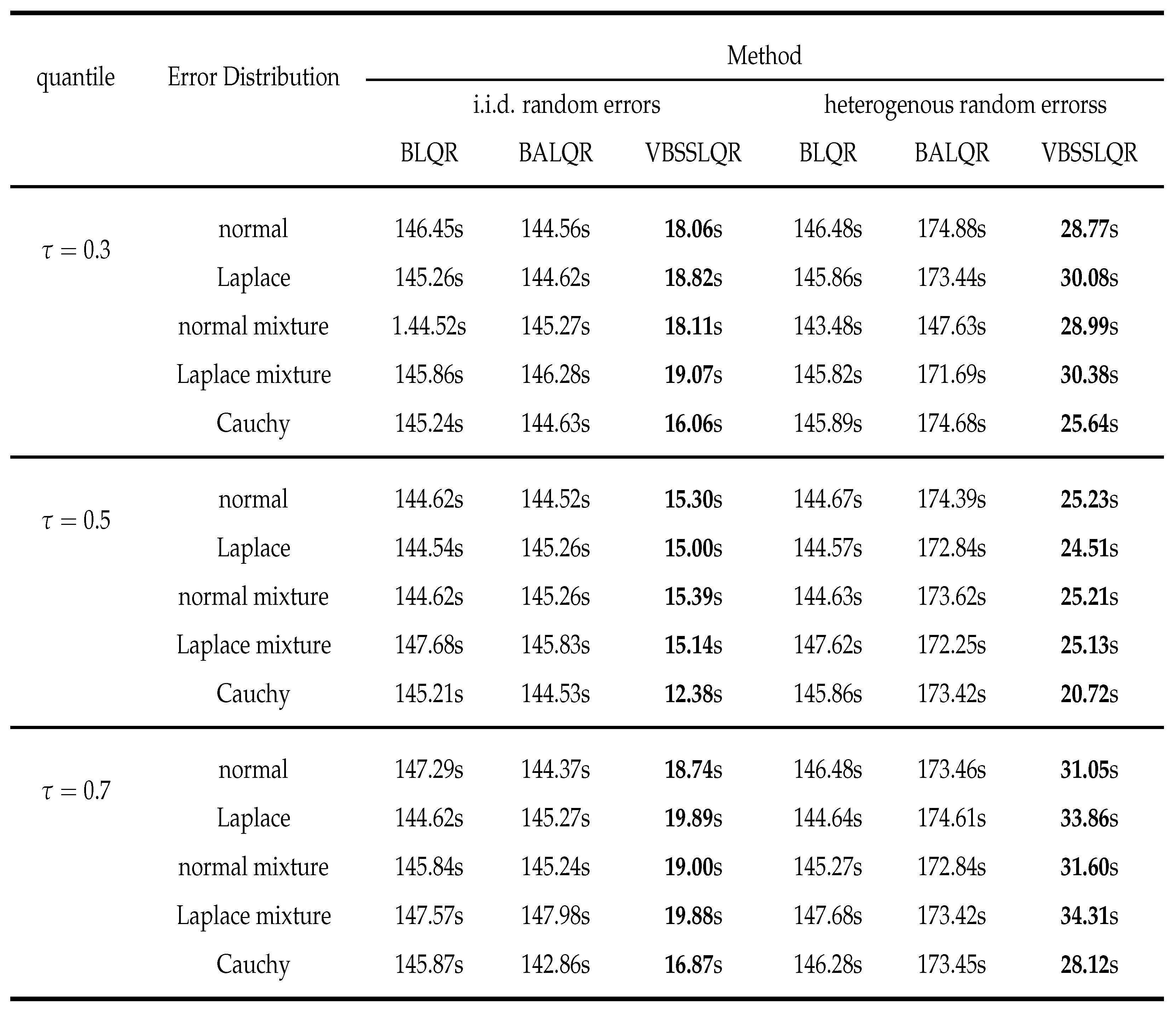
Table A1. Mean execution times of vaious Bayesian quantile regression methods for simulations

References

Koenker, R.; Bassett, G. Regression quantile. Econometrica 1978, 46, 33–50. [Google Scholar] [CrossRef]
Buchinsky, M. Changes in the united-states wage structure 1963-1987 - application of quantile regression. Econometrica 1994, 62, 405–458. [Google Scholar] [CrossRef]
Thisted, R.; Osborne, M.; Portnoy, S.; Koenker, R. The gaussian hare and the laplacian tortoise: computability of squared-error versus absolute-error estimators - comments and rejoinders. Statistical science 1997, 12, 296–300. [Google Scholar]
Koenker, R.; Hallock, K. Quantile regression. Journal of economic perspectives 2001, 15, 143–156. [Google Scholar] [CrossRef]
Yu, K.; Moyeed, R. Bayesian quantile regression. Statistics & probability letters 2001, 54, 437–447. [Google Scholar] [CrossRef]
Taddy, M.A.; Kottas, A. A bayesian nonparametric approach to inference for quantile regression. Journal of business & economic statistics 2010, 28, 357–369. [Google Scholar] [CrossRef]
Hu, Y.; Gramacy, R.B.; Lian, H. Bayesian quantile regression for single-index models. Statistics and computing 2013, 23, 437–454. [Google Scholar] [CrossRef]
Lee, E.R.; Noh, H.; Park, B.U. Model selection via bayesian information criterion for quantile regression models. Journal of the american statistical association 2014, 109, 216–229. [Google Scholar] [CrossRef]
Frank, I.; Friedman, J. A statistical view of some chemometrics regression tools. Technometrics 1993, 35, 109–135. [Google Scholar] [CrossRef]
Tibshirani, R. Regression shrinkage and selection via the lasso. Journal of the royal statistical society, Series B 1996, 58. [Google Scholar] [CrossRef]
Fan, J.; Li, R. Variable selection via nonconcave penalized likelihood and its oracle properties. Journal of the american statistical association 2001, 96, 1348–1360. [Google Scholar] [CrossRef]
Zou, H.; Hastie, T. Regularization and variable selection via the elastic net. Journal of the royal statistical society series b-statistical methodology 2005, 67, 301–320. [Google Scholar] [CrossRef]
Zou, H. The adaptive lasso and its oracle properties. Journal of the american statistical association 2006, 101, 1418–1429. [Google Scholar] [CrossRef]
Koenker, R. Quantile regression for longitudinal data. Journal of multivariate analysis 2004, 91, 74–89. [Google Scholar] [CrossRef]
Wu, Y.; Liu, Y. Variable selection in quantile regession. Statistica sinica 2009, 19, 801–817. [Google Scholar]
Park, T.; Casella, G. The bayesian lasso. Journal of the american statistical association 2008, 103, 681–686. [Google Scholar] [CrossRef]
Leng, C.; Tran, M.N.; Nott, D. Bayesian adaptive Lasso. Annals of the institute of statistical mathematics 2014, 66, 221–244. [Google Scholar] [CrossRef]
Li, Q.; Xi, R.; Lin, N. Bayesian regularized quantile regression. Bayesian analysis 2010, 5, 533–556. [Google Scholar] [CrossRef]
Alhamzawi, R.; Yu, K.; Benoit, D.F. Bayesian adaptive Lasso quantile regression. Statistical modelling 2012, 12, 279–297. [Google Scholar] [CrossRef]
Ishwaran, H.; Rao, J. Spike and slab variable selection: frequentist and bayesian strategies. Annals of statistics 2005, 33, 730–773. [Google Scholar] [CrossRef]
Ray, K.; Szabo, B. Variational bayes for high-dimensional linear regression with sparse priors. Journal of the american statistical association 2022, 117, 1270–1281. [Google Scholar] [CrossRef]
Yi, J.; Tang, N. Variational bayesian inference in high-dimensional linear mixed models. Mathematics 2022, 10. [Google Scholar] [CrossRef]
Xi, R.; Li, Y.; Hu, Y. Bayesian quantile regression based on the empirical likelihood with spike and slab priors. Bayesian analysis 2016, 11, 821–855. [Google Scholar] [CrossRef]
Koenker, R.; Machado, J. Goodness of fit and related inference processes for quantile regression. Journal of the american statistical association 1999, 94, 1296–1310. [Google Scholar] [CrossRef]
Tsionas, E. Bayesian quantile inference. Journal of statistical computation and simulation 2003, 73, 659–674. [Google Scholar] [CrossRef]
Rockova, V. Bayesian estimation of sparse signals with a continuous spike-and-slab prior. Annals of statistics 2018, 46, 401–437. [Google Scholar] [CrossRef] [PubMed]
Alhamzawi, R.; Ali, H.T.M. The bayesian adaptive lasso regression. Mathematical biosciences 2018, 303, 75–82. [Google Scholar] [CrossRef]
Parisi, G.; Shankar, R. Statistical field theory. Physics today 1988, 41, 110. [Google Scholar] [CrossRef]
Beal, M.J. Variational algorithms for approximate bayesian inference. Phd thesis university of london 2003. [Google Scholar]
Kuruwita, C.N. Variable selection in the single-index quantile regression model with high-dimensional covariates. Communications in statistics-simulation and computation 2021. [CrossRef]

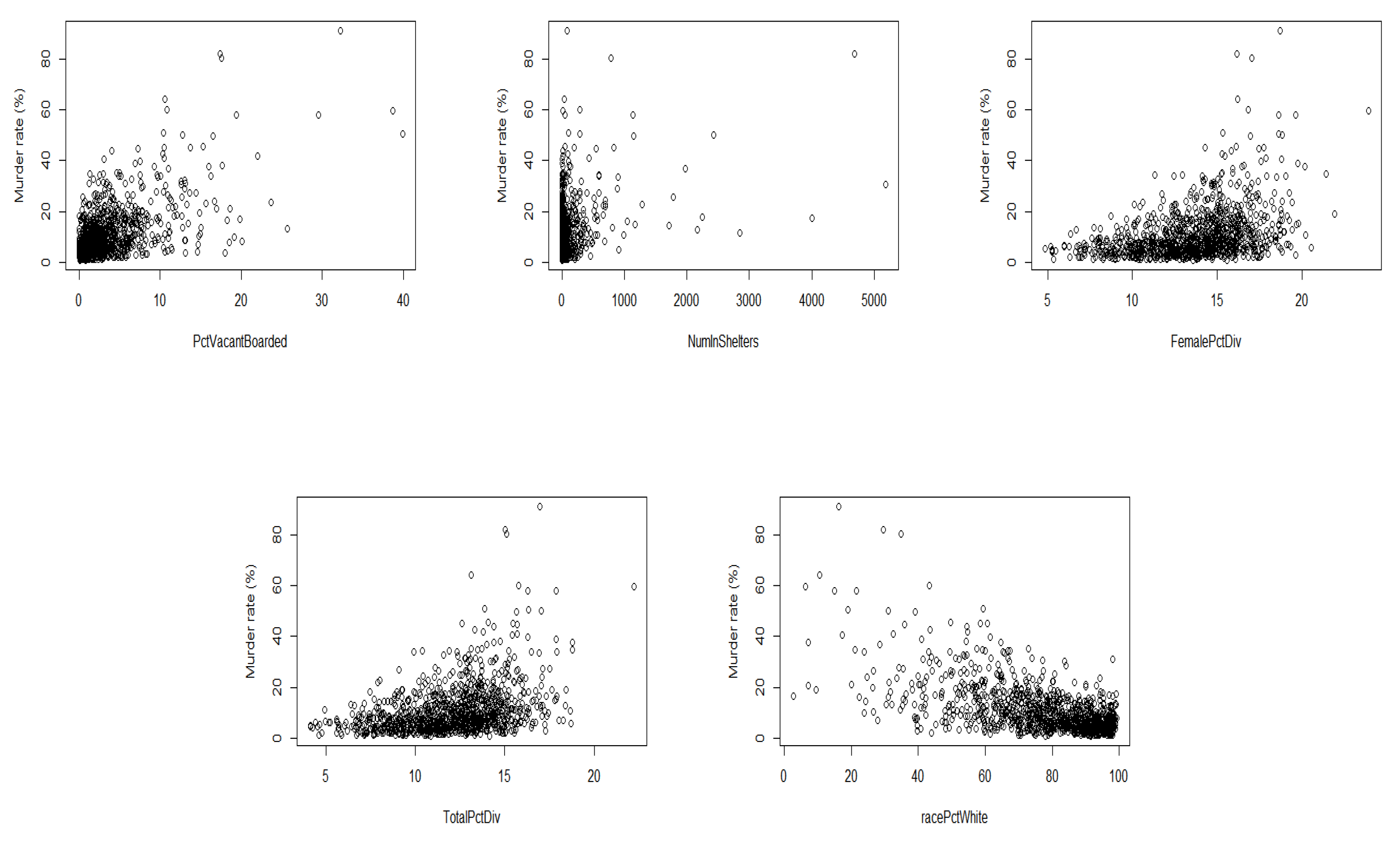
Figure 1. Correlation between murder rate and common variables.

Table 1. The Median and standard deviation of 500 MADs estimated via various methods for simulations with i.i.d. errors.

Table 2. Mean TP/FP of various methods for simulations with i.i.d. errors.

Table 4. Mean TP/FP of various methods for simulations with heterogenous random errors.

Table 5. RMSE of fitting test dataset and the number of active variables of various methods for real dataset

Table 6. Crime data analysis: variable selection.

Disclaimer/Publisher’s Note: The statements, opinions and data contained in all publications are solely those of the individual author(s) and contributor(s) and not of MDPI and/or the editor(s). MDPI and/or the editor(s) disclaim responsibility for any injury to people or property resulting from any ideas, methods, instructions or products referred to in the content.

© 2023 by the authors. Licensee MDPI, Basel, Switzerland. This article is an open access article distributed under the terms and conditions of the Creative Commons Attribution (CC BY) license (http://creativecommons.org/licenses/by/4.0/).

Copyright: This open access article is published under a Creative Commons CC BY 4.0 license, which permit the free download, distribution, and reuse, provided that the author and preprint are cited in any reuse.

MDPI Initiatives

Important Links

Choose an area of interest and we will send you notifications of new preprints at your preferred frequency.

Disclaimer

High-Dimensional Variable Selection for Quantile Regression based on Variational Bayesian Method

Abstract

1. Introduction

2. Models and Methods

2.1. Quantile Regression

2.2. Bayesian Quantile Regression based on Spike-and-Slab Lasso

2.3. Quantile Regression with Spike-and-Slab Lasso Penalty Based on Variational Bayesian

3. Simulation Studies

3.1. Independent and Identically Distributed Random Errors Random

3.2. Heterogenous Random Errors

4. Examples

5. Conclusions

Author Contributions

Funding

Institutional Review Board Statement

Informed Consent Statement

Data Availability Statement

Conflicts of Interest

Appendix A. Deduction

Appendix B. Expectation

Appendix C. Efficiency comparison between Bayesian quantile regression

References

MDPI Initiatives

Important Links

Subscribe