1. Introduction

2. Intraday market

Table 1. Information on submitted orders.

3. The optimization problem

4. Proposed market model

4.2. Bid simulator

The bid simulator has the task of creating the agents, give them the possibility to submit an offer at a certain time, decide the quantity and the price of the offer and adjust their strategy following the market conditions.

4.2.1. Agent creation

For each agent, four characteristics are defined:

• the identification number (I), an integer number varying in the range [1,$N\_max$] with $N\_max$ the maximum number of agents
• the kind of the agent (a), an integer number varying in the range [0, 9] (from 0 to 4 for buyers and from 5 to 9 for sellers)
• the volume of energy (MWh) that an agent wants to buy (sell) in the ID market;
• the ‘private value’ ($p_v$) defined as the maximum (minimum) price (€/MWh) that a buyer (seller) is willing to spend (accept) for buying (selling) energy.

The I number is assigned at the beginning of the algorithm, and it is useful to understand which players obtained the best results at the end of the simulation. The five typologies of buyers and sellers are:

• dispatchable generators that need to buy or sell energy to don’t incur in penalty imbalances;
• dispatchable generators that could buy or sell energy to earn more money;
• non-dispatchable generators that are willing to enter in the market;
• non-dispatchable generators that want to earn more money taking the risk to get penalties imbalances;
• agents that submit offers very close to the equilibrium price of the market.

The volume of energy is a constant quantity and agents submit a slice of it every time they decide to place an order. The private value is calculated with the following procedure: a random number extrapolate from historical prices of imbalance penalties

$$p_{vs}={\alpha }_s·{\Delta }_{imb}$$

(2)

$$p_{vb}={\alpha }_b·{\Delta }_{imb}$$

(3)

With ${\alpha }_sϵ[1,1.3]$ and ${\alpha }_bϵ\left[\mathrm{0.7,1}\right]$. And ${\Delta }_{imb}$calculates as indicate in Table II.

Table 1. Methodology of unbalanced prices.

Table 1. Methodology of unbalanced prices.

	Agent positive unbalancing	Agent negative unbalancing
Zonal positive unbalancing	Agent receives: $Min(P_{dam},Min{P}_{mb})$	Agent pays: $P_{dam}$
Zonal negative unbalancing	Agent receives: $P_{dam}$	Agent pays: $Max(P_{dam},Max{P}_{mb})$

So, agents with a positive imbalance can sell energy and they will be remunerated at the day-ahead market price ($P_{dam}$) if he is bidding in a zone with negative unbalancing while he will be remunerated at the minimum price between the day-ahead market price and the balancing market price ($P_{mb}$) if the bidding zone presents a positive unbalancing. On the contrary, agents with negative imbalances will pay $P_{dam}$ if they are bidding in a positive unbalancing zone or the maximum price between $P_{dam}$ and $P_{mb}$ if they are bidding in a zone with negative unbalancing.

The other three variable parameters are assigned to the agents in order to develop our algorithm properly for an energy market model. These variables are the number of submissions (n), the remaining quantity of energy ($r_q$) to buy or sell and the aggressiveness ($A_g$). n and $r_q$ are important indices for agent submission strategy of an order. Aggressiveness is a key parameter to model price strategy of players inspired by the adaptive-aggressiveness (or AA) strategy [17] and it is the key characteristic that agent uses to lead their behavior as well as the ‘genes’ of the population that NSGA-II modifies to find the optimal solutions. It is defined as the inclination to be more active in the market. An aggressive agent submits better bids than the equilibrium price, increasing the chance of find a match but renouncing big profits. On the other hand, a passive player submits bids worse than the equilibrium price taking the risk to not reach a match but trying to find a more profitable transaction. For instance, an aggressive seller (buyer) will submit offers with a lower (higher) price than the equilibrium one while a passive seller (buyer) will present offers with a higher (lower) cost than the equilibrium price. High level of aggressiveness has a range between 0 and 1: $A_gϵ\left[\mathrm{0,1}\right]$ while low level of aggressiveness has a range between -1 and 0: $A_gϵ[-\mathrm{1,0}]$

4.2.2. Offer submission

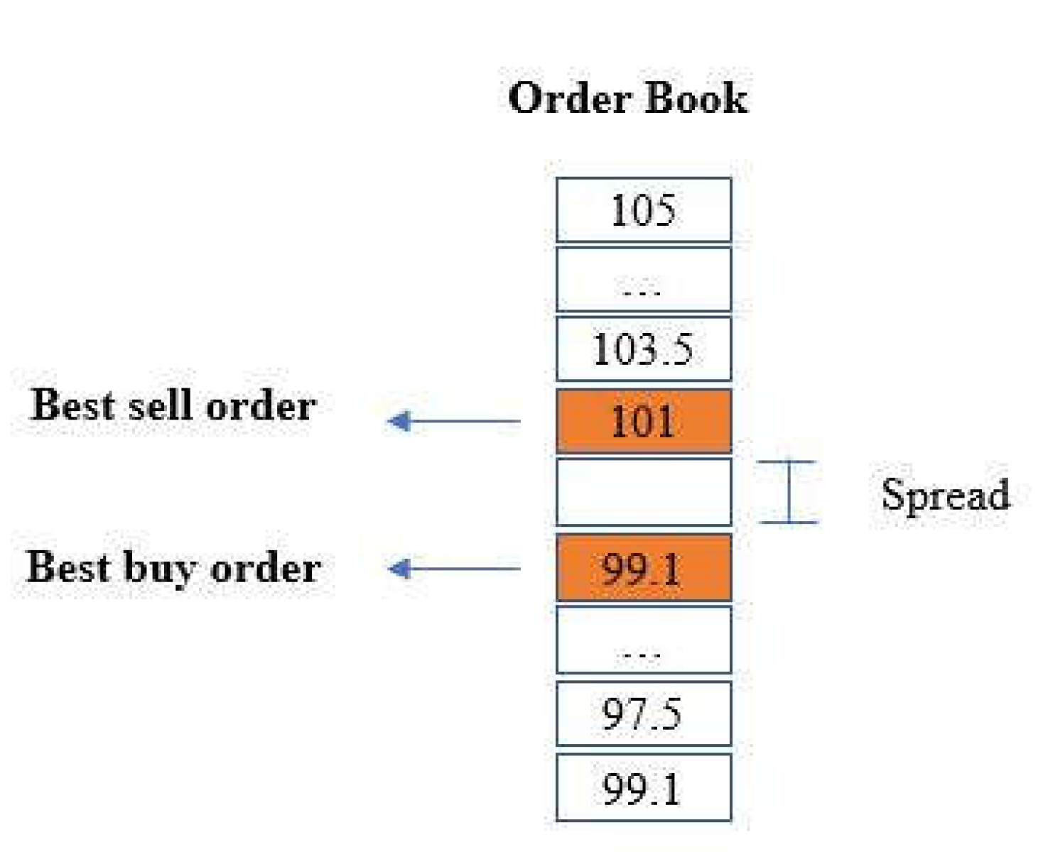
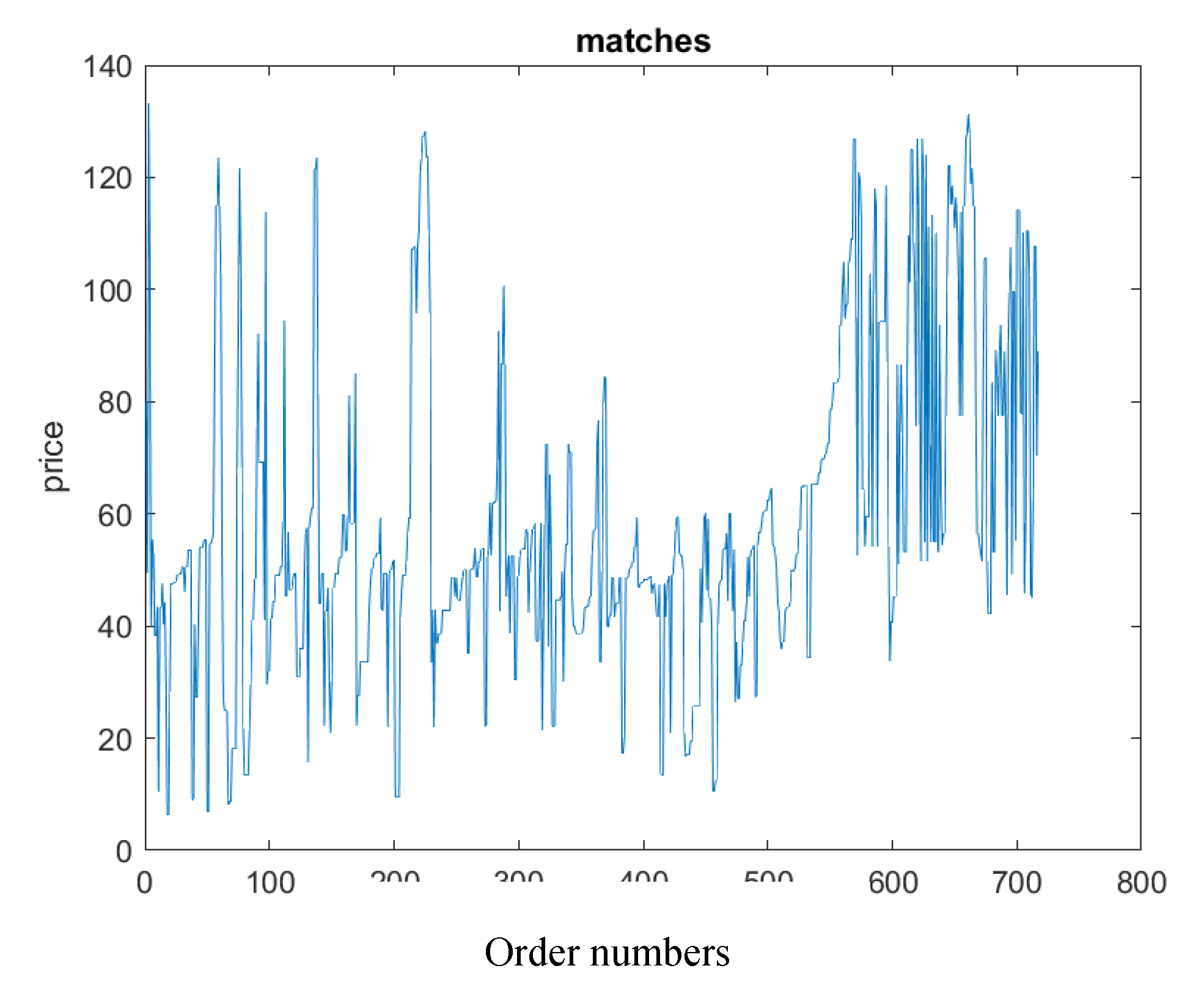
In the SIDC the trading starts one hour after the closing of day-ahead market at $t_{open}$ and end one hour before the delivery time at $t_{close}$ so we call the trading time: ${T=[t_{open},t}_{close}]$. In our model we discretize the continuous trading time into different step $\Delta t$. At each time step an agent is selected by the system and he can decide whether buy or sell an amount of energy or not. The agent’s selection is made by three different methods: randomly, following the average match prices or depending on the quantity submitted. The random method is the easiest and it is also the one that give more random results: the algorithm selects casually an identify number and the associated agent decide whether submit a bid or not as showed in the algorithm1. Let’s give some notation to facility the reading of the algorithm: ${Sb}_i$ indicate the player’s i decision of submission, $V_i^{max}$is the total volume of the agent i, and $V_i$ is the volume submitted by the agent i. $P_i$ is the price submitted by the agents i, $P_m$ is the equilibrium market price, $P_{av}$ is the price average of the last 5 matches as maximum, $p_{bb}$ and $p_{bs}$ are respectively the best buy order and the best sell order present in the order book and maxP is the maximum price offer allows in the market.

Algorithm 1: random selection of a participant

1: Open order book $\Delta t$= $t_{open}$2: while $\Delta t$ < $t_{close}$ do

3: agent= rand (I)

4: Order: $O_i(V_i,P_i)$5: Sending the order to the order book

6: Update agent’s strategy

7: end while

8: Close order book

Point 3 of algorithm 1 can be set with other two methods mentioned before. In particular:

Algorithm 1.1: selection depending on the average matched prices

3: for $\Delta t$<10

3.1: agent= rand (I)

3.2: end for

3.3: Calculation of match price average:

$$P_{av}=\frac{{\displaystyle {\sum }_{i=1}^{N_5\_macth}{P}_{matches}}}{N_{matches}}$$

(4)

3.4: if $P_{av}$< $P_m$

3.5: agent= 75% buyer, 25% seller

3.6: else

3.7: agent= 75% seller, 25% buyer

3.8: end for

This procedure states that when the market price ($P_{av}$) is lower than the equilibrium market price, buyers are more willing to enter in the market trying to find a more profitable deal, while $P_{av}$is higher than the equilibrium price, sellers enter in the market to gain better revenues.

Algorithm 1.2: selection depending on the volume submitted

3: for $\Delta t$<10

3.1: agent= rand (I)

3.2: end for

3.3: Percentage of the volume submitted over total volume for all agents

3.4: for i=1: number of agents

$$V_s=\frac{V_i}{V_i^{max}}$$

(5)

3.5: end for

3.6: agent= choose by a vector of probabilities depending on $V_s$

In this method the agent with the highest probability to be selected is the one who presents the lowest value of $V_s$. This happens because an agent who has not been able to sell/buy its volume of energy is more willing to submit an offer than agents who have already sold the majority of the volume. Agent selection is chosen at the beginning of the analyses, and it cannot be changed by NSGA-II algorithm, but it is useful to represent different scenarios of continuous market.

4.2.3. Choice of the volume

The mechanism by which an agent decides the volume of a bid doesn’t follow a real strategy. Each round it submits a quantity in between the 10 and 20% of its total quantity. Analyzing data of German ID market of transaction occurred in 2020 [29] we saw that most of the traders preferred to submit a lot of order with a small quantity of energy volume (around 5MWh). For this reason, in our model all players submit just a small part of the entire capacity at every submission time. When an agent finishes its quantity, he cannot be called by the system until the end of the simulation. When all agents finish their quantity, the simulation stops. The amount of energy submitted by each agent is not considered a key parameter for these analyses because it is supposed that volumes to buy or sell is known a priori at the beginning of the market session by all agents, and consequently it is not affected by the NSGA-II algorithm.

4.2.4. Order prices

The agent’s formulation of prices follows the AA strategy [17] of the continuous double auction (CDA) [28] and it is enhanced by the introduction of the NSGA-II algorithm. In fact, in order to comply the objective functions regarding the welfare and the unsold quantity, agents must be able to submit their bids with the optimal price in a certain market timeframe. For instance, following the market results, a seller will decide whether to enter in the market presenting a high price offer (that could increase his welfare while taking the risk to not find a bid in the opposite direction) or to submit a low-price offer that increase the possibility to sell his imbalance volume. These analyses show how the NSGA-II algorithm is able to optimize the agent’s decision in the session of continuous market. The price formulation is also strictly dependent to the characteristics of the power plant. The function used to generate prices is continue and dependent to the aggressiveness $A_g$ and ϴ that represents the magnitude of the gradient [30]. For the fivekinds of agents previously mentioned we defined 5 different strategies for buyers and 5 for sellers (for all strategies: if the match average price has not been already calculated $p_{av}=p_m$ ):

Strategy 1b: dispatchable buyer generator with high risk of imbalances due to a breakdown

1: set initial aggressive ($A_g$) value between [0.6;1]

2: if buyers’ book-depth is empty

3: price $p_i=p_{av}+\left(pv-p_{av}\right)\mathrm{*}\left(\frac{e^{ag\mathrm{*}ϴ}-1}{e^{ϴ}-1}\right)$ (6)

4: if buyers’ book is not empty

5: $p_i={\mathrm{m}\mathrm{a}\mathrm{x}(p}_{av};p_m,;p_{bb})+\left(pv-{\mathrm{m}\mathrm{a}\mathrm{x}(p}_{av};p_m,;p_{bb})\right)\mathrm{*}\left(\frac{e^{ag\mathrm{*}ϴ}-1}{e^{ϴ}-1}\right)$ (7)

These generators that need to buy/sell energy are power plant that faced a breakdown after the closing of day-ahead market and cannot respect the bids previously accepted so they want to be sure to enter in the ID market to adjust their position even without obtaining big revenues.

Strategy 2b: dispatchable buyer generator that buys energy only if the trade is highly profitable.

1: set initial aggressive ($A_g$) value between [-1; -0.6]

2: if buyers’ book-depth is empty

3: price $p_i=p_{av}\mathrm{*}\left(1-\frac{e^{-ag\mathrm{*}ϴ}-1}{e^{ϴ}-1}\right)$ (8)

4: if buyers’ book is not empty

5: price $p_i={\mathrm{m}\mathrm{i}\mathrm{n}(p}_{av};p_m,;p_{bb})\mathrm{*}\left(1-\frac{e^{-ag\mathrm{*}ϴ}-1}{e^{ϴ}-1}\right)$ (9)

These are dispatchable generators that could buy/sell energy in the market. They are already balanced but with the possibility to produce or take more energy from the market with high costs. So, they decide to enter only if obtaining big revenues.

Strategy 1s: dispatchable seller generator with high risk of imbalances due to a breakdown

1: set initial aggressive ($A_g$) value between [0.6;1]

2: if sellers’ book-depth is empty

3: price $p_i=pv+\left(p_{av}-pv\right)\mathrm{*}\left(1-\frac{e^{ag\mathrm{*}ϴ}-1}{e^{ϴ}-1}\right)$ (10)

4: if sellers’ book is not empty

5: price $p_i=pv+\left({\mathrm{m}\mathrm{i}\mathrm{n}(p}_{av};p_m,;p_{bs})-pv\right)\mathrm{*}\left(1-\frac{e^{ag\mathrm{*}ϴ}-1}{e^{ϴ}-1}\right)$ (11)

This strategy refers to the strategy 1b but for sellers.

Strategy 2s: dispatchable seller generator that sells energy only if the trade is highly profitable

1: set initial aggressive ($A_g$) value between [-1; -0.6]

2: if sellers’ book is empty

3: price $p_i=p_{av}+\left(maxP-p_{av}\right)\mathrm{*}\left(\frac{e^{-ag\mathrm{*}ϴ}-1}{e^{ϴ}-1}\right)$ (12)

4: if sellers’ book is not empty

5: $p_i={\mathrm{m}\mathrm{a}\mathrm{x}(p}_{av};p_m,;p_{bs})+\left(maxP-{\mathrm{m}\mathrm{a}\mathrm{x}(p}_{av};p_m,;p_{bs})\right)\mathrm{*}\left(\frac{e^{-ag\mathrm{*}ϴ}-1}{e^{ϴ}-1}\right)$ (13)

This strategy refers to the strategy 2b but for sellers

For non-dispatchable generators, formulas for bids prices are the same of the dispatchable generators. The main differences are the initial aggressiveness and the possibility to switch from an aggressive strategy to a passive one and vice-versa depending on the market conditions. We report the strategies of a non-dispatchable buyer that starts active and a non-dispatchable seller that starts passive. The strategies adopted respectively buy passive buyer and active follows the same rules

Strategy 3b: non-dispatchable buyer generator

1: set initial aggressive ($A_g$) value between [0; 1]

2: price $p_i=p_{av}+\left(pv-p_{av}\right)\mathrm{*}\left(\frac{e^{ag\mathrm{*}ϴ}-1}{e^{ϴ}-1}\right)$ (14)

3: processing the bid in the order book

4: update $A_g$

5: if $A_g$>0 restart from point 2

6: else, price $p_i=p_{av}\mathrm{*}\left(1-\frac{e^{-ag\mathrm{*}ϴ}-1}{e^{ϴ}-1}\right)$ (15)

Strategy 4s: non-dispatchable seller generator

1: set initial aggressive ($A_g$) value between [-1; 0]

2: price $p_i=p_{av}+\left(maxP-p_{av}\right)\mathrm{*}\left(\frac{e^{-ag\mathrm{*}ϴ}-1}{e^{ϴ}-1}\right)$ (16)

3: processing the bid in the order book

4: update $A_g$

5: if $A_g$)<0 restart from point 2

6: else, price $p_i=pv+\left(p_{av}-pv\right)\mathrm{*}\left(1-\frac{e^{ag\mathrm{*}ϴ}-1}{e^{ϴ}-1}\right)$ (17)

Strategies 3b and 4s represent dispatchable generators with the characteristics of switching between an aggressive to a passive behavior. This represents the hard forecast of energy production for a no-programmable resource that has to face the random climate conditions.

The last type of agent introduced are the one who submits bids only following the market equilibrium price, that statistically [17] is the price at which most of the match occurred. For this type of player, the aggressiveness is not necessary

Strategy 5: non-dispatchable seller or buyer generator

$$p_i=p_m*(0.8+0.4*rand)$$

(18)

They want to buy/sell energy without a particular strategy, but they submit bids focusing on the fact that the majority of transactions takes place around the prices that come out form the day-ahead market [23].

For four typologies of agents out of five, the aggressiveness is the parameter that defines the prices of their bids and that is the reason why it is set as the ‘gene’ of each individual in the NSGA-II simulation.

4.2.5. Submission of a bid

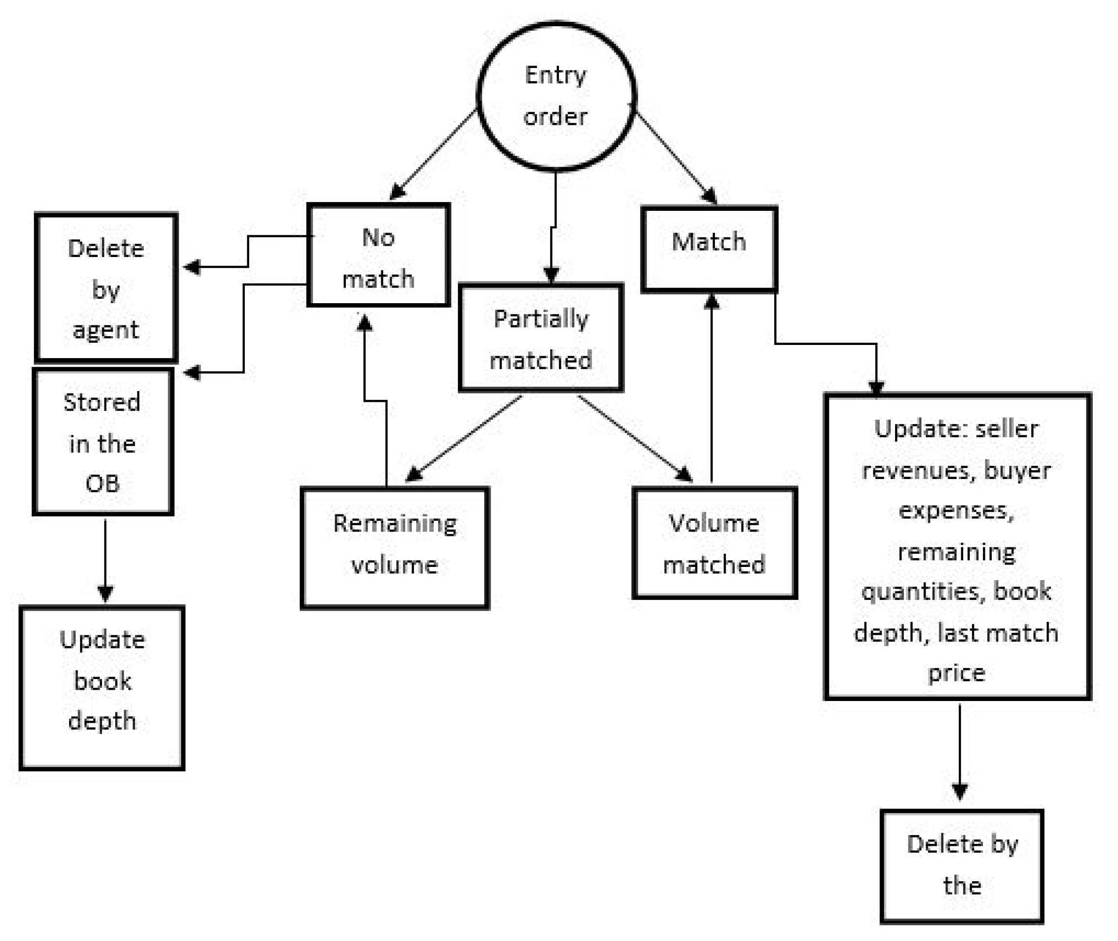
In [29] is stated that most of the bids submitted are then deleted by agents and only a small percentage remain in the order book. To replicate this trading in our model we introduced the possibility to delete a bid submitted upon the occurrence of certain conditions. Algorithm 2 explains the agent’s decision:

Algorithm 2: decision to submit or delete a bid for buyer

1: if buyers’ book is empty submit bid

2: if $p_i>p_{av}*(1-\mathsf{\epsilon })$ submit bid else don’t submit

3: bid processing in the order book

4: if no-match occurs and if sellers’ book > ψ delete bid

5: if no-match occurs and if sellers’ book <= ψ don’t delete bid

Algorithm 2.1: decision to submit or delete a bid for seller

1: if sellers’ book is empty submit bid

2: if $p_i<p_{av}*(1+\mathsf{\epsilon })$ submit bid else don’t submit

3: bid processing in the order book

4: if no-match occurs and if buyers’ book > ψ delete bid

5: if no-match occurs and if buyers’ book <= ψ don’t delete bid

Where ε is a parameter in the range [0;1] that determine the choice of an agent if submitting or not depending on how far the position of the bid in the order book ranking is. An ε close to 1 increases the willingness of submission while an ε close to 0 decreases the willingness of submission. Ψ is aositive value that determine the choice of deleting a bid stored in the order book or not. For example, if a seller submits a bid, it is not matched and ψ=5 it means that there are five buy bids that cannot be matched with the one just submitted due to its high price. So, it is hard that the bid will find a match later and it is better to delete it and submit another one.

4.2.6. NSGA-II Optimization strategy

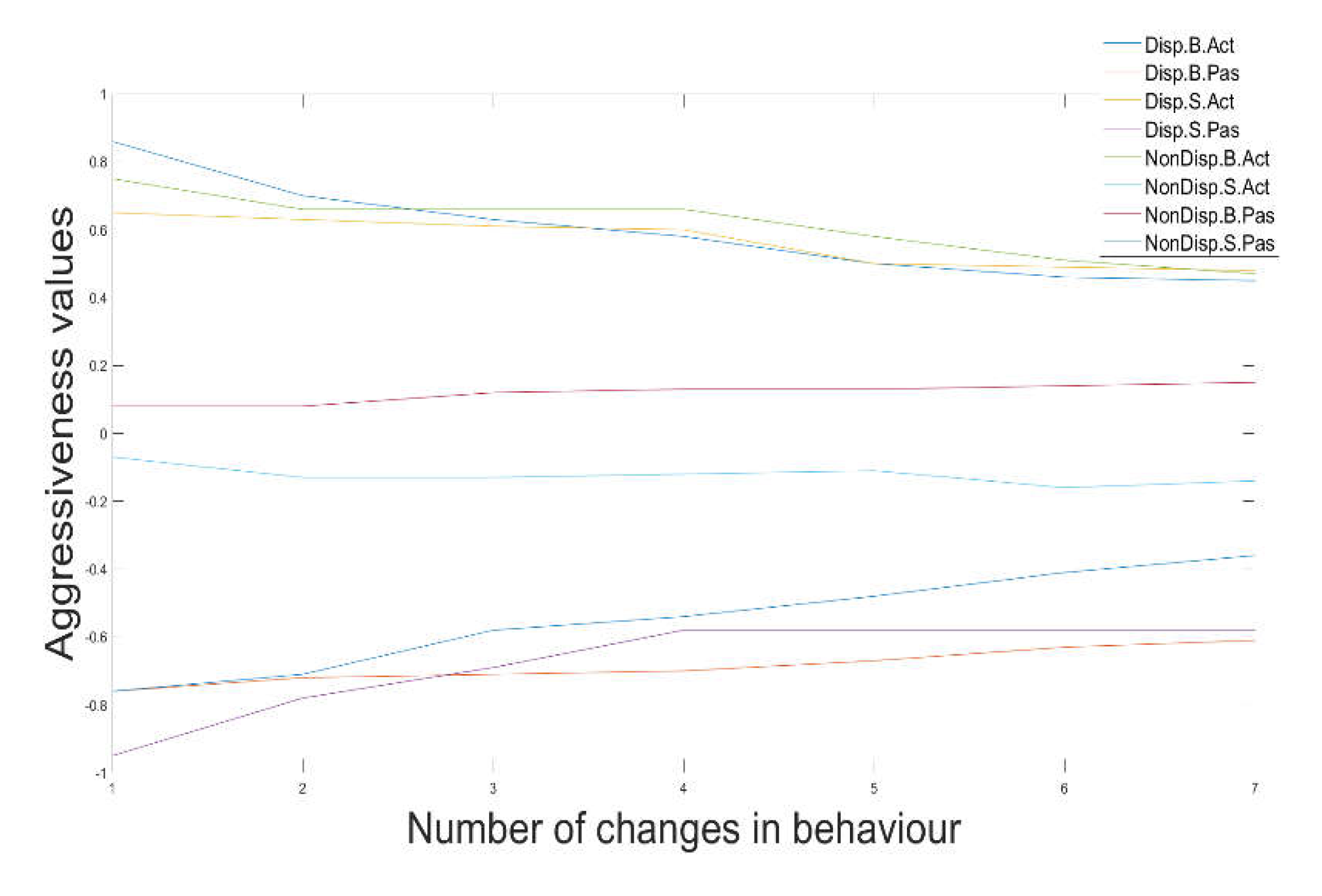
Each agent starts the market session with a given level of aggressiveness ($A_g$ ϵ [-1; 1]) and can modify this level following the market events. In more detail, an aggressive agent that find a match can decide to decrease his aggressiveness to obtain a match with bigger revenues and on the other hand, a passive agent that does not find a match can decide to increase his aggressiveness to have more chance to enter in the market. The general aim of anagent is to obtain the optimal level of aggressiveness that enables to enter in the market and maximize the profits. In our model we first replicated the method presented by Vytellingum et all. [17] to regulate agents’ aggressiveness and secondly, we compared the results with a model that use genetic algorithm to update the same parameters. 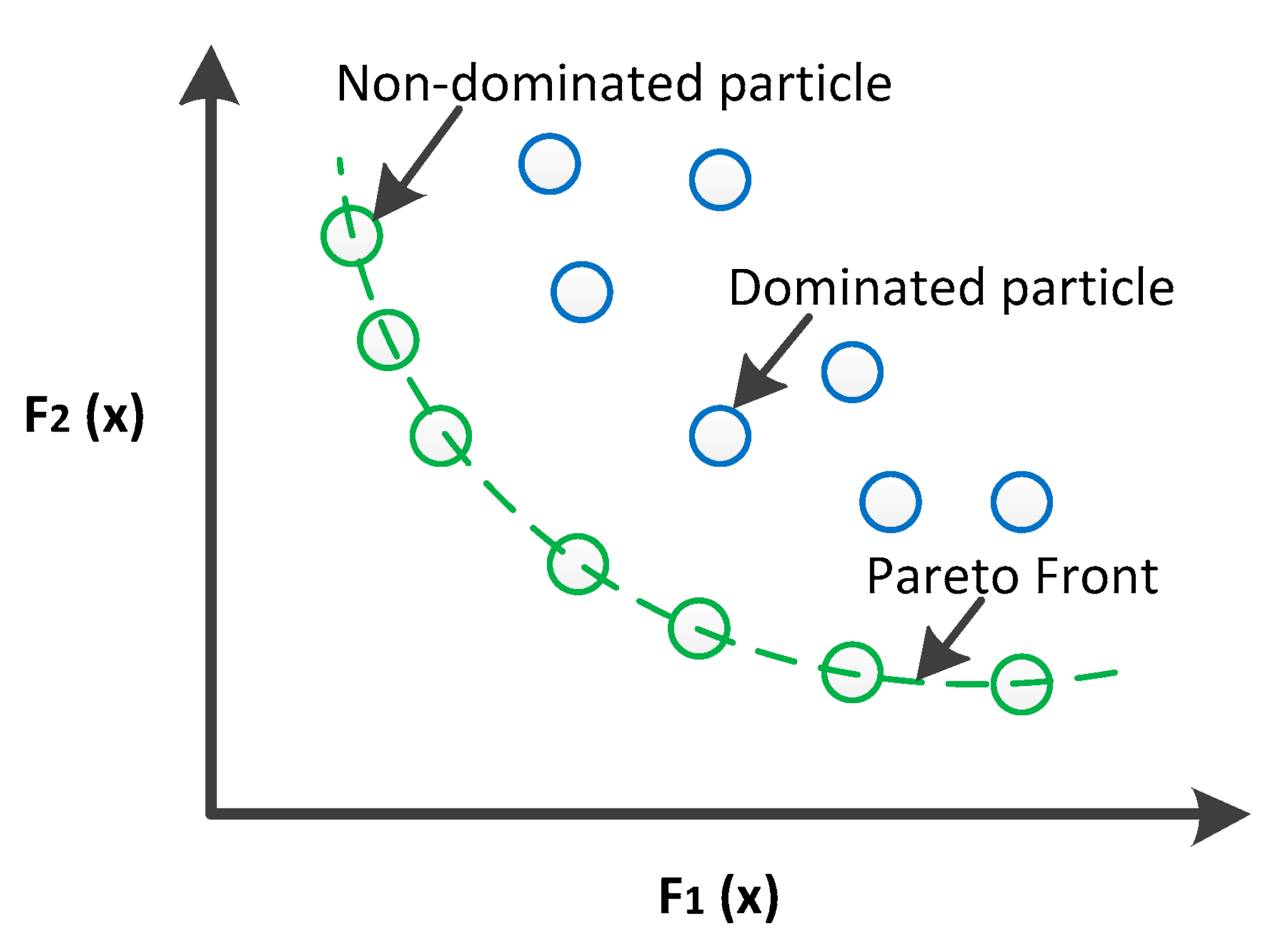In particular we introduced the non-dominating sorting genetic algorithm (NSGA-II) implemented based on [31] defining two objective functions and a set of variables. Here the NSGA-II is described and explained how it can be applied to our model. The algorithm that simulates the ID market is composed by different phases fundamental to determine how the NSGA-II suits in the context. In fact, every time one generation starts, different market sessions are launched characterized by agents with different peculiarities described in section 4.1 and all individuals (market players) trade among themselves until the market session is finished. Results of each market session depict the welfare of the system, the welfare of buyers and sellers and the unsold quantity that cause imbalances. These are the objectives functions better described further on. Obviously, most of the characteristics of the market are fixed and NSGA-II does not interact with them so the market can be replicated properly. The optimization algorithm will be applied only to aggressiveness characteristic that define the behavior adopted by agents and highlights their strategies defined in section 4.4.

Now all the parameters that we set in the NSGA-II algorithm to be combined with our model are described. The process starts with different sets of players who represent the population. Each set of players is characterized by a set of variables (aggressiveness) individually associated to a player. Thus, variables are scalar values joined into a string to form the solution. How fit is a set of players is evaluated thanks to the objective functions. The algorithm gives a score to the set of individuals to represent the probability to be selected for reproducing and pass the characteristics of aggressiveness to the next set of players. A high score gives more chance to the set of players to be selected for reproducing. For each pair of set of players to be coupled a crossover point is chosen randomly within the sets of aggressiveness and the next generation sets of players are created by exchanging the aggressiveness of the previous sets among themselves until the crossover point is achieved. At this point the new set of players is added to the set of population. When a new set of players is formed, a mutation may occur. This mince that some of the aggressiveness in the new set of players can be changed. The process ends when the sets of aggressiveness converge so there are not significative differences between a set of players and the next one ore when the number of generations is completed by the program. In the following section the objective functions used to determine which are the best sets of aggressiveness that players must utilize to trade in the continuous ID market is described.

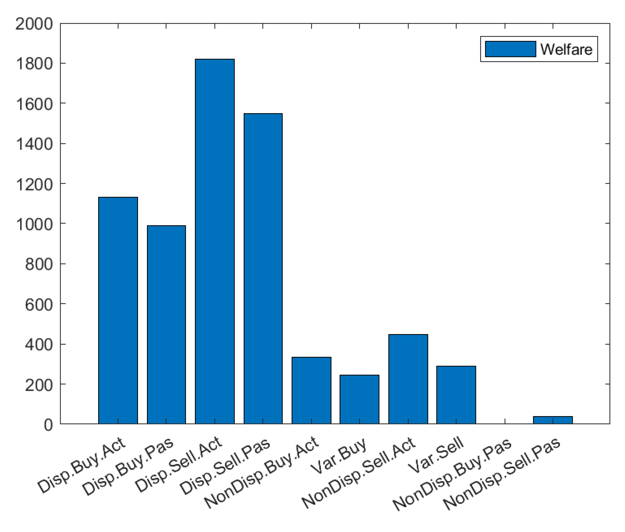
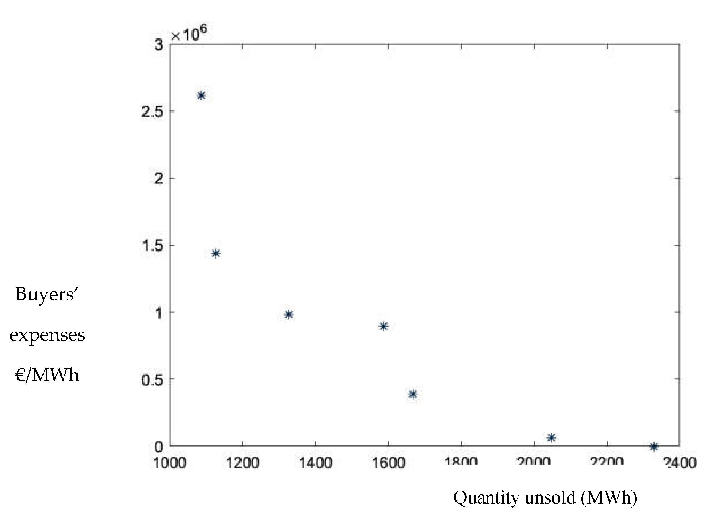
At this point the objective functions are described. Analysis has been focused on the optimization of functions regard the welfare of the agents, the total welfare and the unsold quantity which is the source of penalty imbalances in the market. For each optimization, only two of the aforementioned objective functions have been considered. For instance, the welfare of buyers (related to their expenses) and the unsold quantity are optimized at the same time to find out what is the best compromise of aggressiveness that allows to deliver big amounts of energy without incurring in prices higher and lower compared to the market price. The objective functions considered two by two, depending on the optimization problem to solve, are the following:

A. Welfare sellers

This function represents the revenues of the sellers in respect of what they are expecting to gain. It has to be maximized.

$$W_s=\sum _{i=1}^{N.sellers}{q}_m^i\mathrm{*}(p_m^i-p_o^i)$$

(19)

B. Welfare buyers

This function represents the savings of buyers in respect to what they are willing to spend. It has to be maximized.

$$W_b=\sum _{i=1}^{N.buyers}{q}_m^i\mathrm{*}(p_0^i-p_m^i)$$

(20)

C. Total welfare

This function represents the general welfare of the system. It has to be maximized

$$W_{tot}=W_s+W_b$$

(21)

D. Remaining volumes

This function represents the total volumes that agents have not been able to exchange in the market. It has to be minimized.

$$V_r=\sum _{i=1}^{n.agents}{V}_i^{max}-V_i$$

(22)

Where $q_m^i$, $p_m^i$ and $p_o^i$ are respectively the quantity matched the price of the match the price of the submission of player i.

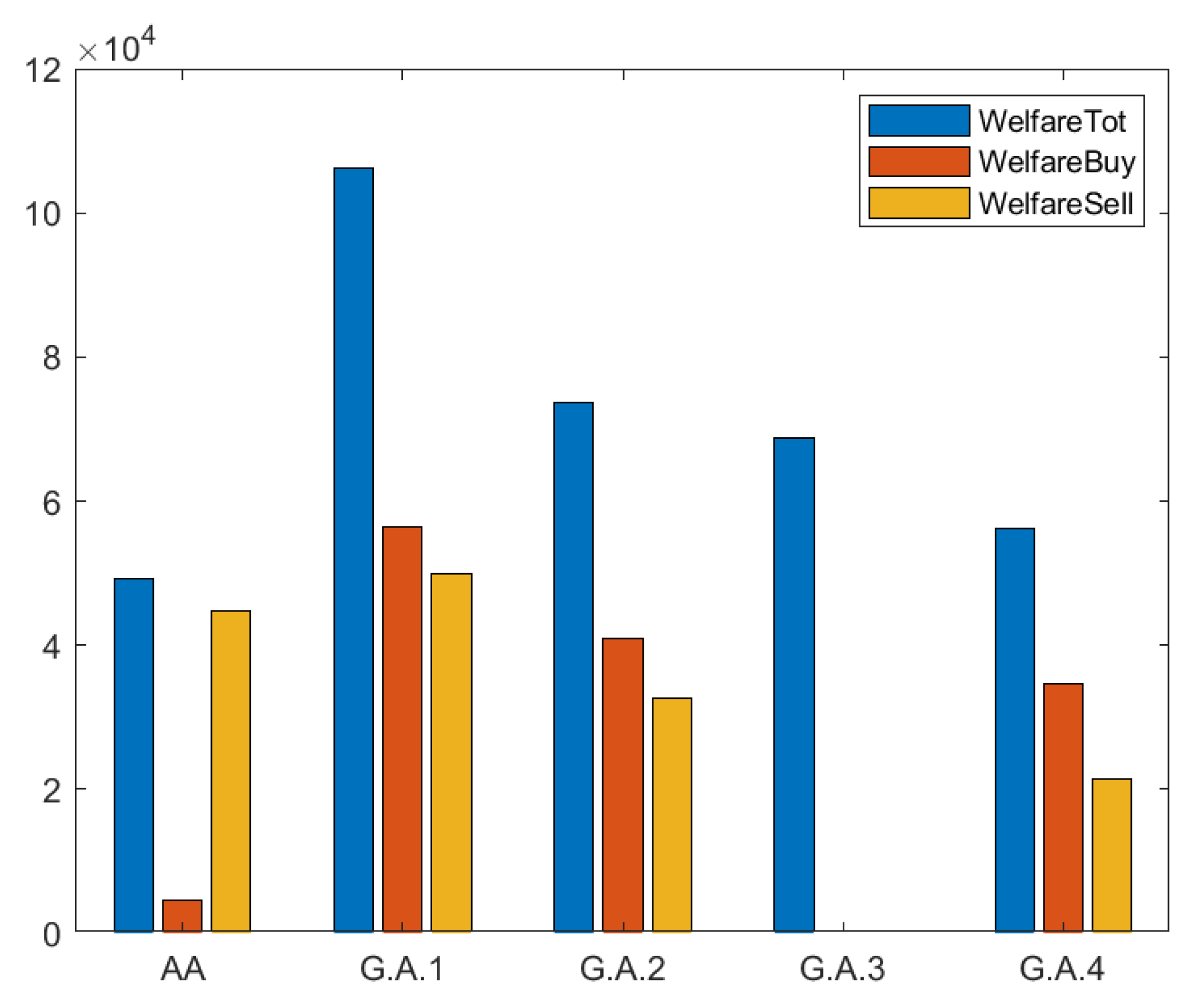
For every generation a set of aggressiveness is assigned to the population divided equally into sellers and buyers, and the objective functions are calculated. The best set of individuals are the ones that obtain the highest welfare, or the lowest unsold quantity and they get the lowest rank and the highest crowding distance into NSGA-II. The process continues until the end of the generations as previously mentioned. The combination of different objective function has been led to analyze four different problems to evaluate the market efficiency:

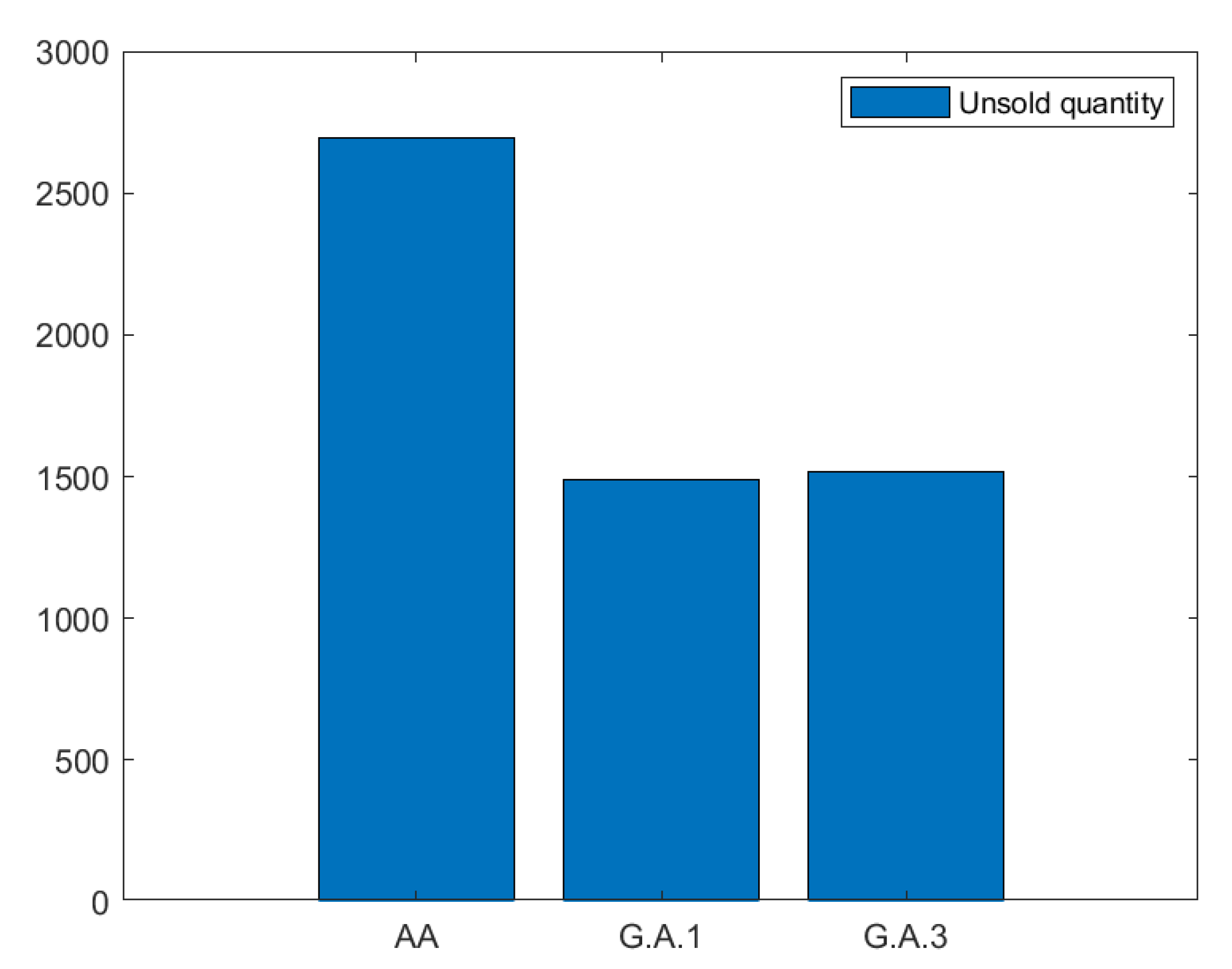
• Problem 1:(G.A.1) wants to maximize the buyers and sellers’ welfare and minimize the unsold quantity.
• Problem 2: (G.A.2) wants to maximize the buyers and sellers’ welfare only.
• Problem 3: (G.A.3) aims at maximizing the total welfare and minimizing the unsold quantity
• Problem 4: (G.A.4) tries to maximize at the same time the buyers, sellers, and total welfare.

5. Results

5.2. Results with genetic algorithm

In this section we show how the use of NSGA-II algorithm modifies the results in terms of welfare and volumes sold compared to the simple AA-method. In these analyses we want to solve a multi-objective problem and consequently the solution is not unique. We find a set of optimal solutions reported in the Pareto front [33]. The method is very useful since it gives the opportunity to better understand the system exploring the consequences of different decisions with respect to the objectives [34]. In the first optimization using NSGA-II a scenario with eight players (one for each kind excluding the buyer and seller of strategy 5) is considered. The trading lasts for 100 steps, selected following algorithm 1.1. The set of aggressiveness is the variable modified by the algorithm for each generation and the objective functions are the unsold quantity and the buyers’ expenses. Both functions must be minimized. In Figure 8 we plot the Pareto front with the unsold volumes on x-axis and the buyers’ expenses on y-axes.

The set of solutions varies from zero expenses for buyers, but no volumes exchanged to almost all volumes exchanged with high expenses for buyers. In table III we report the values of the set of aggressiveness that lead to the solutions obtained in Figure 8.

Table 3. Values of aggressiveness and the corresponding objective functions.

Table 3. Values of aggressiveness and the corresponding objective functions.

Set	${\mathit{A}}_{\mathit{g}1}$	${\mathit{A}}_{\mathit{g}2}$	${\mathit{A}}_{\mathit{g}3}$	${\mathit{A}}_{\mathit{g}4}$	${\mathit{A}}_{\mathit{g}5}$	${\mathit{A}}_{\mathit{g}6}$	${\mathit{A}}_{\mathit{g}7}$	${\mathit{A}}_{\mathit{g}8}$	Unsold volume (MWh)		Expenses (€/MWh)
1	0.15	0.19	-0.21	-0.71	0.83	-0.92	-0.57	-0.72	2328	0	1
2	0.13	0.29	-0.17	-0.60	0.83	-0.87	-0.75	-0.71	1088	2618491	2
3	0.13	0.36	-0.17	-0.59	0.84	-0.89	-0.74	-0.62	2328	0	3
4	-0.52	-0.52	0.25	-0.06	0.16	-0.52	-0.65	0.70	1128	1440241	4
5	-0.53	-0.55	0.24	-0.05	0.17	-0.54	-0.64	0.68	1328	985245	5
6	0.15	0.18	-0.19	-0.74	0.82	-0.91	-0.57	-0.62	1668	389589	6
7	0.13	0.35	-0.17	-0.59	0.84	-0.89	-0.74	-0.62	2048	64209	7
8	0.15	0.19	-0.21	-0.71	0.83	-0.92	-0.57	-0.72	1588	893321	8

We can notice that the optimal solutions are always characterized by 5 passive and only three active agents. Among these, 4 over 5 are very passive (less than -0.5) and 1 over three is very active (more than 0.5). Since the aggressivity from $A_{g1}$ to $A_{g1}$ refer to buyers while from $A_{g5}$ to $A_{g8}$ refer to seller it seems that the Pareto front is obtained when among buyers there are two active players, one passive and one very passive while among sellers there are three passive and one very aggressive. This means that the best solution is not achieved when players turn their strategy pricing energy around the equilibrium price as we have seen with the AA method.

6. Results

References

1. European commission. EU action. Available online: https://climate.ec.europa.eu/eu-action/international-action-climate-change/climate-negotiations/paris-agreement_en (accessed on 20 August 2022).
2. ENTSO-E. Power statistics. Available online: https://www.entsoe.eu/data/power-stats/ (accessed on 22 August 2022).
3. European Commission, Directorate-General for Energy, Schumacher, L., Küpper, G., Henneaux, P., et al., The future electricity intraday market design, Publications Office, 2019. [CrossRef]
4. Neuhoff, Karsten, et al. Intraday Markets for Power: Discretizing the Continuous Trading. Energy Policy Research Group, University of Cambridge, 2016. JSTOR. https://www.jstor.org/stable/resrep30358.
5. ACER Electricity and gas retail markets volume, ACER market monitoring report, 2018.
6. ENTSOE. Single intraday coupling (SIDC). Available online: https://www.entsoe.eu/network_codes/cacm/implementation/sidc/ (accessed on 25 August 2022).
7. Maurício T. Tolmasquim, Tiago de Barros Correia, Natália Addas Porto, Wikus Kruger,Electricity market design and renewable energy auctions: The case of Brazil,Energy Policy,Volume 158,2021,112558,ISSN 0301-4215. [CrossRef]
8. J. Bellenbaum, M. Bucksteeg, T. Kallabis, C. Weber Intraday cross-zonal capacity pricing. Paris, 2016.
9. Henriot, Arthur. “Market Design with Centralized Wind Power Management: Handling Low-Predictability in Intraday Markets.” The Energy Journal, vol. 35, no. 1, 2014, pp. 99–117. JSTOR. https://www.jstor.org/stable/24693820.
10. Anke, Weidlich and Veit Daniel, (2008), Agent-Based Simulations for Electricity Market Regulation Advice: Procedures and an Example, Journal of Economics and Statistics (Jahrbuecher fuer Nationaloekonomie und Statistik), 228, (2-3), 149-172. [CrossRef]
11. N.R. Jennings, An agent-based approach for building complex software sys- tems, Commun. ACM 44 (4) (2001) 35–41. [CrossRef]
12. T. Nagata and H. Sasaki, "A multi-agent approach to power system restoration," in IEEE Transactions on Power Systems, vol. 17, no. 2, pp. 457-462, May 2002. [CrossRef]
13. Cliff, Dave. “Minimal-Intelligence Agents for Bargaining Behaviors in Market-Based Environments.” (1997).
14. Gode, Dhananjay K., and Shyam Sunder. “Allocative Efficiency of Markets with Zero-Intelligence Traders: Market as a Partial Substitute for Individual Rationality.” Journal of Political Economy, vol. 101, no. 1, 1993, pp. 119–37. JSTOR. https://www.jstor.org/stable/2138676.
15. Steven Gjerstad, John Dickhaut,Price Formation in Double Auctions,Games and Economic Behavior,Volume 22, Issue 1,1998,Pages 1-29,ISSN 0899-8256. [CrossRef]
16. Tesauro, Gerald and Jonathan Bredin. “Strategic sequential bidding in auctions using dynamic programming.” AAMAS '02 (2002). [CrossRef]
17. P. Vytelingum, D. Cliff, N.R. Jennings,Strategic bidding in continuous double auctions, Artificial Intelligence,Volume 172, Issue 14,2008,Pages 1700-1729,ISSN 0004-3702. [CrossRef]
18. B. Widrow and M. E. Hoff, “Adaptive Switching Circuits,” 1960 IRE WESCON Convention Record, 1960, pp. 96-104.
19. Eur Lex. Official website of the European Union. Available online: https://eurlex.europa.eu/legalcontent/EN/TXT/?uri=CELEX%3A32015R1222 (accessed on 01 September 2022).
20. EPEXSPOT. Epexspot Operational Rules. Available online: https://www.epexspot.com/en/regulation (accessed on 30 August 2022).
21. NEMO Committee. Public description of continuous trading match algorithm. Available online: https://www.ote-cr.cz/cs/kratkodobe-trhy/integrace-trhu/files-xbid/public-description-of-continuous-trading-matching-algorithm.pdf (accessed on 5 September 2022).
22. OMIE. Details of intraday market operation. Available online: https://www.omie.es/sites/default/files/inlinefiles/intraday_and_continuous_markets.pdf (accessed on 5 September 2022).
23. Alberizzi, A. Zani, P. Di Barba, M., Pantos, " Statistical analysis of two different intraday market designs: the German and Iberic intra-day market," 2022 18th International Conference on the European Energy Market (EEM). [CrossRef]
24. K. Deb, Multi-Objective Optimisation Using Evolutionary Algorithms, Wiley, 2001. [CrossRef]
25. J.R.Manne ‘Swarm intelligence for multi-objective optimization in engineering design’. Advanced Methodologies and Technologies in Artificial Intelligence, Computer Simulation, and Human-Computer Interaction, page 15. [CrossRef]
26. Kumar, Mahesh & Nallagownden, Perumal & Elamvazuthi, Irraivan. (2016). Advanced Pareto Front Non-Dominated Sorting Multi-Objective Particle Swarm Optimization for Optimal Placement and Sizing of Distributed Generation. Energies. 9. 982. [CrossRef]
27. Journal Articl,e Deep Reinforcement Learning, P. Aske arXiv preprint arXiv:2201.02135 2022. [CrossRef]
28. Shinde P, Boukas I, Radu D, Manuel de Villena M, Amelin M. Analyzing Trade in Continuous Intra-Day Electricity Market: An Agent-Based Modeling Approach. Energies. 2021; 14(13):3860. [CrossRef]
29. Alberizzi, A. Zani and P. Di Barba, " Analysis of the intraday market: statistical analysis of German single intraday coupling” 2022 AEIT International Annual Conference (AEIT), 2022. [CrossRef]
30. Vytelingum, Perukrishnen. “The structure and behaviour of the continuous double auction.” (2006).
31. Vytelingum, P., Dash, R.K., David, E. and Jennings, N. R. (2004) A risk-based bidding strategy for continuous double auctions. 16th European Conference on Artificial Intelligence, 79-83, Valencia, Spain.
32. K. Deb, A. Pratap, S. Agarwal and T. Meyarivan, "A fast and elitist multiobjective genetic algorithm: NSGA-II," in IEEE Transactions on Evolutionary Computation, vol. 6, no. 2, pp. 182-197, April 2002. [CrossRef]
33. Miguel Martínez-Iranzo, Juan M. Herrero, Javier Sanchis, Xavier Blasco, Sergio García-Nieto,Applied Pareto multi-objective optimization by stochastic solvers,Engineering Applications of Artificial Intelligence,Volume 22, Issue 3,2009,Pages 455-465,ISSN 0952-1976. [CrossRef]
34. P. Hilber, V. Miranda, M. A. Matos and L. Bertling, "Multiobjective Optimization Applied to Maintenance Policy for Electrical Networks," in IEEE Transactions on Power Systems, vol. 22, no. 4, pp. 1675-1682, Nov. 2007. [CrossRef]