
Submitted:
18 April 2023
Posted:
19 April 2023
You are already at the latest version
Abstract
As development progresses, when the bottom hole flowing pressure or formation pressure is less than the saturation pressure of crude oil in the reservoir, oil and gas two-phase seepage occurs in the reservoir. Due to the characteristics of oil and gas two-phase seepage, after the oil and gas two-phase seepage occurs in the reservoir, the well production will be reduced, or even greatly reduced. Therefore, how to predict the horizontal well capacity better in this case is an important problem that needs to be solved urgently. In this paper, the method and process of establishing the transient calculation model of two-phase flow in horizontal wells are introduced in detail from three aspects: fluid physical properties, reservoir oil-gas two-phase seepage, and the coupling model of Inflow Performance and Flow in Wellbore. The model is more reliable through the verification of production data from five wells in two oilfields.
Keywords:
horizontal well
; capacity prediction
; transient model
; saturation pressure
; two-phase seepage
1. Introduction
Productivity prediction is an important task in the development of horizontal wells. When the well bottom flowing pressure or formation pressure is less than the saturation pressure of formation crude oil, oil and gas two-phase seepage will occur in the reservoir and wellbore, and the prediction model will be more complicated.
In 1958, Merkulov [1,2] published an article for the first time, proposing a formula for calculating horizontal well production. He assumed that the reservoir shape was box-shaped and the horizontal well was located in the center of the reservoir, and then used the seepage mechanics method to derive the production formula of the horizontal well under steady seepage conditions. In 1964, Borisovsy [3] systematically summarized the development process of horizontal wells and inclined wells, introduced the production principle of horizontal wells, and comprehensively applied seepage mechanics principle and mathematical derivation methods to obtain the yield analysis formula of horizontal wells under steady seepage conditions. In 1984, Giger [4,5,6] used basically the same assumptions as Borisov’s formula to derive the oil recovery index equation for a horizontal well in the center of the reservoir. In the same year, he proposed the formula for calculating the horizontal well capacity of heterogeneous reservoirs, which is obtained by replacing the original permeability with equivalent permeability on the basis of the homogeneous reservoir capacity formula. The Giger equation, like Borisov’s equation, does not take into account the limitations of horizontal length of horizontal wells and ignores the effect of wellbore pressure drop.
In 1986, Joshi [7,8,9] established a single-phase seepage model of horizontal wells based on the principle of electric field flow. This model simplifies the three-dimensional ellipsoid seepage problem of horizontal wells, simplifies it into two two-dimensional seepage problems in the horizontal plane and vertical plane, and uses potential energy theory to derive the steady-state productivity equation of horizontal wells in homogeneous isotropic reservoirs. Assumptions: (1) single-phase, steady-state flow; (2) weakly compressible fluid; (3) homogeneous oil reservoir, without considering skin effect ; (4) The outer boundary is the constant pressure boundary; (5) The horizontal well is located in the middle of the reservoir. In 1988, Babuproposed the productivity equation for horizontal wells in the box-type closed reservoir he studied. This productivity equation is different from the productivity equation of other scholars and considers the quasi-steady flow. In 1990, Renard and Dupuy studied the impact of formation damage on horizontal wells based on the summary of the productivity equation of Joshi and Giger horizontal wells, and obtained the productivity equation of horizontal wells considering skin effect. The equation is suitable for circular oil drainage area, elliptical oil drainage area and rectangular oil drainage area.
In 1996, Dou Hongenregarded the horizontal well as a vertical well across an infinite formation, and derived the horizontal well capacity formula according to the potential superposition principle. In 1996, Shedid explored the difference of seepage mechanism between heel and toe of horizontal section of horizontal well, and described the shape of the oil drainage area of horizontal wells through two rectangles and a semicircle. After a series of studies, he proposed a horizontal well oil production index formula applicable to gas cap and bottom water reservoirs. In 2008, based on the research of Joshi and Giger on the production formula of horizontal wells, Chen Yuanqian [13,14] used the area equivalence method to equivalently convert the elliptical oil drainage area to a quasi-circular oil drainage area, at the same time, changed the length of the horizontal section into a quasi-circular production tunnel according to the principle of production equivalence, and finally obtained a new horizontal well production calculation formula by using the equivalent flowing resistance method. In 2010, Liu Wenchaodivided the ellipsoid of horizontal wells into inner zone, middle zone and outer zone, derived the steady seepage capacity calculation formula of the corresponding area according to the seepage characteristics of each zone, and finally obtained the production formula for calculating the horizontal well in heavy oil reservoir according to the fluid flow through the boundary of each zone is equal.
In 2019, based on the analysis of typical seepage characteristics of horizontal wells, Jia Xiaofeiet al. considered the planar elliptical flow and deduced a new comprehensive productivity formula of horizontal wells by using the water and electricity similitude principle and the equivalent flowing resistance method. This formula is more adaptable than the commonly used formula, and can calculate the horizontal well capacity under different drainage shapes, penetration ratios, etc. In 2021, Gao Yihuaet al., based on the potential superposition principle and the mirror reflection principle, established the calculation model of radial flow distribution along the wellbore of horizontal wells across plugging faults under two modes, obtained the Productivity prediction method of horizontal well cross fault in complex fault-block oilfield, and on this basis, formed a reservoir engineering method to quickly optimize the sectional length of horizontal wells across plugging faults in each fault block.
However, most of the research results of predecessors are based on steady-state and single-phase, which can no longer meet the needs of the current development and construction of smart oilfields. Based on this, this paper studies the transient model of horizontal well capacity prediction coupled with oil and gas two-phase seepage and wellbore flow, and the studied model is verified by analogy with the existing model.
2. Establishment of Oil and Gas Two-phase Seepage and Its Coupling Model with Wellbore
According to the basic principle of reservoir oil and gas seepage, the basic equation of oil and gas two-phase seepage can be obtained. For the oil phase, there is:
For the gas phase, there is:
Where and are the relative permeability of oil and gas, which are functions of oil saturation . and are the volume factor and viscosity of the oil phase, which are functions of pressure. , and are the volume factor, viscosity and dissolved gas-oil ratio of the gas, which are also functions of pressure.
From equations (1) and (2), it can be seen that the functions to be solved are pressure and saturation , but in the two equations, the coefficient terms are often functions of these two functions, so such an equation has a strong nonlinearity, and at the same time, the obtained solutions (such as pressure and saturation) have a strong dependence on these state parameters (such as relative permeability, volume factor, dissolved gas-oil ratio, viscosity, etc).
The establishment of the above equation implies that the pressure of the oil layer is lower than the saturation pressure of crude oil, so there will be oil and gas two-phase seepage in the formation, so the above two equations exist. Since the oil layer pressure is lower than the original saturation pressure, with the continuous degassing of crude oil, the properties of crude oil such as crude oil volume coefficient and viscosity and dissolved gas-oil ratio are changed.
2.1. Simplified model - calculation of fluid physical properties under average pressure conditions in a certain region segment
The basic equation of two-phase seepage in oil and gas is a nonlinear partial differential equation, which is commonly solved by approximate methods. Based on the assumptions of the material balance method:
(1) At any moment, the porosity, fluid saturation and relative permeability of the reservoir are uniform;
(2) Regardless of the gas zone and oil zone in the reservoir, the formation pressure is the same, and the volume coefficient, viscosity and gas dissolution amount of gas and oil are the same;
(3) Regardless of the influence of gravity;
(4) At any moment, the oil phase and the gas phase are balanced;
(5) No water intrusion, not counting the amount of water output.
Rs, Bo, and Bg are all functions of the average formation pressure P, determined by high-pressure physical property experiments, as shown in Figure 1.
Production GOR:
Since the production gas-oil ratio is the ratio of the gas flow (including dissolved gas and free gas) converted to standard conditions to the oil flow rate converted to standard atmospheric conditions, the production gas-oil ratio can also be written as:
Where is the gas flow rate under oil layer conditions, , cm3/s. is the oil flow rate under oil layer conditions, , cm3/s. , are the viscosity of gas and oil, which are functions of the average formation pressure , mPa·s.
The relationship between average formation pressure and formation oil saturation can be obtained by equating the above two equations:
In the above formula, the viscosity of crude oil and natural gas are also functions of pressure, as shown in Figure 2.
According to the above formula, the saturation of formation crude oil under different average formation pressure conditions can be obtained, and the relationship between the recovery degree and the average formation pressure can be further obtained, as shown in Figure 3.
2.2. Simplified model - calculation of average pressure in a certain region segment
Using steady-state sequential replacement method:
Each instantaneous moment of the whole process of unsteady oil and gas two-phase seepage can be approximated as a steady state, and the unsteady state of the whole process can be regarded as a superposition of many steady states.
From the relationship curve between average formation pressure and formation crude oil saturation, the pressure can be divided into several intervals, and the pressure value and saturation value in each interval are taken as the median value:
In each small pressure interval, it is considered that the oil and gas seepage is steady, and the physical characteristics of the internal fluid are consistent.
2.3. Calculation of H (potential) of three-dimensional spatial horizontal well under the condition of oil-gas two-phase flow
When the gas-mixed oil seepages into the well under the dissolved gas drive mode, its flow state is unsteady, and the well production (or bottom hole pressures) changes with time. However, considering that although the process of gas-mixed oil seepage is unsteady, at every moment in the total process can be approximately regarded as a steady state.
That is to say, in a certain short period of time, the formation pressure and oil saturation change little. If this time interval is small enough, it can be considered that the pressure and saturation are independent of time. That is steady seepage. At this time, the oil well production formula obtained according to the steady state will basically conform to the actual situation.
Corresponding to the oil-gas-water two-phase flow, although the oil has been produced, the oil-phase flow always exists throughout the production process. Therefore, it is more appropriate to consider the flow process in the oil-gas-water three-phase with the phase seepage law of the oil phase. Seepage law of oil phase can refer to the method of single-phase oil seepage law in literature (Liu P, et al.) [18]. The instantaneous (one sink point in space) production (under the ground conditions) is:
Importing , we can get
If , then
Compare the single-phase spatial steady-state point sink function and the single-phase spatial instantaneous point source function:
Then it can be seen that the instantaneous point sink function of the oil phase in the oil and gas two-phase is:
Similarly, single-phase seepage can obtain the spatial instantaneous line sink function of oil and gas two-phase and the calculation function of horizontal well H (potential) in different types of reservoirs, as well as the coupling model and solution method.
That is, the H (potential) generated by an entire horizontal segment on space(,,) is:
The H (potential) on the right side of the equation is obtained by calculating and accumulating several intervals separately.
Oil well productivity prediction is also closely related to the types of reservoirs. Different types of reservoirs have different potentials in the formation for each segment of the horizontal well. The bottom water reservoir is taken as an example for illustration, other reservoir calculations can be deduced by referring to the literature Liu Xiangping [19], et al. Assuming that the reservoir type of the two-phase seepage of oil and gas is upper and lower closed boundary reservoir, the calculation method of horizontal well H (potential) in the upper and lower closed boundary reservoir is as follows.
2.4. Calculation of Spatial Potential of Uniform Inflow into Horizontal Section in Closed Reservoir
For the upper and lower closed boundary reservoir as shown in Figure 4, a horizontal well with length is divided into segments.
According to the mirror reflection principle, as shown in Figure 5, we can get:
where is the potential generated by the j-th line sink at any point in the oil layer; is the flow rate of the j-th line sink; is the oil thickness; is the between each part of the well and the bottom of the oil layer; is a constant; and is the function defined by the following formula:
where are the length of the j-th segment line sink; and are the start and end abscissas of the j-th segment line in the x-axis direction, and the other parameters are and directions coordinates.
That is, the H (potential) generated by a certain horizontal segment on space (,,) is:
2.5. Horizontal Well Flow Relationship
According to the potential superposition principle, the potential generated by the whole horizontal well in the oil layer is:
For different types of reservoirs, the formula is respectively equal to the formulas in braces in Equation (19).
It can be obtained from Equation (22).
The formula is the potential function at the constant pressure boundary or oil drain boundary; is the potential generated by the j-segment line sink at the constant pressure boundary or the oil drain boundary.
It is obtained by Equations (22) and (23).
According to the potential function Equation (13), we can obtain
The H (potential) on the left side of the equation can be obtained by regional integration according to Equation ( 13 ) , as follows.
Where is the pressure at any point in the oil layer (or the comprehensive pressure after considering the potential energy difference); is the permeability of the oil layer; is the permeability of the oil phase; is the relative permeability of the oil phase; is the viscosity of crude oil. is the crude oil volume factor.
2.6. Coupling Model of Inflow Performance and Flow in Wellbore and Its Solution
The three-dimensional steady-state seepage of fluid in the oil layer and the flow in the wellbore are both interrelated and affect each other. Suppose the pressure at the midpoint of the section line sink on the horizontal well is , and the potential generated by the section line sink at the midpoint of the section line sink is , the linear equation system for the production of each segment is obtained according to equations (26), (25) and (22), and the production of each segment is obtained by solving the equation.
According to the variable mass calculation method, the pressure drop in the wellbore is calculated, and the pressure at the point of the section in the wellbore is:
Where , is the flowing pressure at the heel end of the wellbore.
The total production of the whole well is
In the above-mentioned coupled model, both and are unknowns, which can be solved using the iterative method.First Assuming a set of values, use equations (26), (25), (22) to solve array .Then, array is substituted into the pressure drop formula and equation (27) to update array from heel to toe Then update array from the linear equation system of formula production , and so on, until both and array reach a certain computational accuracy. Finally, the total well production can be obtained from Equation (29).
3. Example of transient productivity prediction calculation of oil and gas two-phase seepage in horizontal wells
3.1. Samples Calculation
Known conditions:
(1) The basic parameters are shown in Table 1.
(2) The phase penetration data is shown in Figure 6.
(3) The result is shown below.
It can be seen from Figure 7, Figure 8, Figure 9 and Figure 10 that under the same production pressure difference conditions, if it is a single-phase flow, the production is the same. If it is an oil and gas two-phase seepage, the production is lower than that of single-phase flow, and the more serious the degassing, the lower the production. The calculation result is as follows:
3.2. Verification of productivity prediction of two oilfields
In order to test the transient coupling model of the established horizontal well productivity prediction, the IPR prediction verification was carried out by taking the test production horizontal wells in Iran MIS oilfield and the test production horizontal wells in Hafaya oilfield as examples.
(1) MIS oil field, Iran
The basic parameters and test production data of the two wells such as MIS 320 CN-H7 are shown in Table 2, Table 3, Table 4, Table 5 and Table 6, respectively.
The prediction results of different productivity prediction methods of MIS 320 CN-H7 well and the error analysis with the Experimental production data are shown in Figure 11 and Table 7 below, respectively.
The prediction results of different productivity prediction methods of MIS 322 CN-H2 well and the error analysis with the trial production data are shown in Figure 12 and Table 8 below, respectively.
(4) Hafaya oil field
The basic parameters and test production data of the three wells in Hafaya are shown in Table 9, Table 10, Table 11, Table 12, Table 13 and Table 14, respectively.
The prediction results of different productivity prediction methods of HF003-S001H well and the error analysis with the experimental production data are shown in Figure 13 and Table 15 below, respectively.
The prediction results of different productivity prediction methods of HF002-M001H well and the error analysis with the experimental production data are shown in Figure 14 and Table 16 below, respectively.
The prediction results of different productivity prediction methods of HF001-N002H wells and the error analysis with experimental production data are shown in Figure 15 and Table 17 below, respectively.
The absolute average relative error statistics and average error calculation of the five wells are shown in Table 18.
4. Acknowledgments
Thanks to Luo Wei, the corresponding author of this article. This article was funded by the open fund project “Study on transient flow mechanism of fluid accumulation in shale gas wells” of the Sinopec Key Laboratory of Shale Oil/Gas Exploration and Production Technology.
5. Conclusions
(1) The difficulty of transient productivity prediction of oil and gas two-phase seepage in horizontal wells is that after the pressure of the oil layer is lower than the saturation pressure, the volume factor and phase permeability of crude oil change with pressure, which are functions of pressure, and to calculate these parameters, the pressure at this position needs to be calculated. In addition, the calculation of the potential of the horizontal well is also extremely complicated, and it is necessary to consider the parameters of some parameters with the pressure change as a whole to calculate, but it does not hinder the relationship between the horizontal well potential (pressure) and production established by the potential superposition principle, so as to establish a production prediction model with the coupling of formation oil and gas two-phase seepage and wellbore pipe flow.
(2) The calculation example shows that when bottom hole flowing pressure is higher than the saturation pressure, the same production pressure difference will result in the same output; When the bottom hole flowing pressure is lower than the saturation pressure, the oil and gas two-phase seepage occurs in the near well area, and the other areas (higher than the saturation pressure) are still single-phase seepage, and the production decreases. When formation pressure and the bottom hole flowing pressure are further reduced, the two-phase seepage area of the reservoir oil and gas expands, and the production will be greatly reduced.
(3) The model has high applicability, small error and reliable model through the prediction and verification of production from multiple field logs.
References
- Karcher, B.J.; Giger, F.M.; Combe, J. Some Practical Formulas to Predict Horizontal Well Behavior. In Proceedings of the 61st Annual Technical Conference and Exhibition, New Orleans, LA, USA, 5–8 October 1986; SPE Paper 15430; OnePetro: Richardson, TX, USA, 1986. [Google Scholar]
- Lifeng, W.; Chunjiang, C.; Helin, W.; Zeng, N. A review of the development of horizontal well productivity calculation. China Pet. Chem. Ind. 2007, 18, 39–41. [Google Scholar]
- Shedid, A.E.; Samuel, O.O.; Djebbar, T.A. Simple Productivity Equation for Horizontal Wells Based on Drainage Area Concept. In Proceedings of the Western Regional Meeting, Anchorage, AK, USA, 22–24 May 1996; SPE Paper 35713; OnePetro: Richardson, TX, USA, 1996. [Google Scholar]
- Giger, F.M.; Reiss, L.H.; Jourdan, A.P. The Reservoir Engineering Aspects of Horizontal Drilling. In Proceedings of the 59th Annual Technical Conference and Exhibition, Houston, TX, USA, 16–19 September 1984; SPE Paper 13024; OnePetro: Richardson, TX, USA, 1984. [Google Scholar]
- Giger, F.M. Horizontal Wells Production Techniques in Heterogeneous Reservoirs. In Proceedings of the SPE 1985 Middle East Oil Technical Conference and Exhibition, Sakhir, Bahrain, 11–14 March 1985; SPE Paper 13710; OnePetro: Richardson, TX, USA, 1985. [Google Scholar]
- Giger, F.M. Low-Permeability Reservoirs Development Using Horizontal Wells. In Proceedings of the SPE/DOE Low Permeability Reservoirs Symposium, Denver, CO, USA, 18–19 May 1987; SPE Paper 16406; OnePetro: Richardson, TX, USA, 1987. [Google Scholar]
- Joshi, S.D. Augmentation of Well Productivity Using Slant and Horizontal Wells. In Proceedings of the 61st Annual Technical Conference and Exhibition of the Society of Petroleum Engineers, New Orleans, LA, USA, 5–8 October 1986; SPE Paper 15375; OnePetro: Richardson, TX, USA, 1986. [Google Scholar]
- Joshi, S.D. A Review of Horizontal Well and Drainhole Technology. In Proceedings of the 62nd Annual Technical Conference and Exhibition of the Society of Petroleum Engineers, Dallas, TX, USA, 27–30 September 1987; SPE Paper 16868; OnePetro: Richardson, TX, USA, 1987. [Google Scholar]
- Joshi, S.D. Production Forecasting Methods for Horizontal Wells. In Proceedings of the SPE International Meeting on Petroleum Engineering, Tianjin, China, 1–4 November 1988; SPE Paper 17580; OnePetro: Richardson, TX, USA, 1988. [Google Scholar]
- Babu, D.K.; Odeh, A.S. Productivity of a Horizontal Well. SPE Reserv. Eng. 1989, 4, 417–421. [Google Scholar] [CrossRef]
- Renard, G.; Dupuy, J.M. Formation Damage Effects on Horizontal-Well Flow Efficiency. In Proceedings of the 1990 SPE Formation Damage Control Symposium, Lafayette, IN, USA, 22–23 February 1991; SPE Paper 19414; OnePetro: Richardson, TX, USA, 1991. [Google Scholar]
- Dou, H. A New Method of Predicting the Productivity of Horizontal Well. Oil Drill. Prod. Technol. 1996, 18, 76–81. [Google Scholar] [CrossRef]
- Chen, Y.-Q. Derivation and Correlation of Production Rate Formula for Horizontal Well. Xinjiang Pet. Geol. 2008, 29, 68–71. [Google Scholar]
- Chen, Y.-Q.; Guo, E.-P. Query, Derivation and Comparison About Joshi’s Production Rate Formula for Horizontal Well in Anisotropic Reservoir. Xinjiang Pet. Geol. 2008, 29, 331–334. [Google Scholar]
- Liu, W.; Tong, D.; Zhang, S. A new method for calculating productivity of horizontal well in low-permeability heavy oil reservoir. Acta Pet. Sin. 2010, 31, 458–462. [Google Scholar]
- Jia, X.; Sun, Z.; Lei, G. A new comprehensive formula for productivity prediction of horizontal well. Oil Drill. Prod. Technol. 2019, 41, 78–82. [Google Scholar]
- Gao, Y.; Zhang, Y.; Yang, B.; Li, K.; Yuan, Z.; Kang, B.; Zhang, X.; Zhang, X.; Chen, G. Productivity prediction and optimization method of segment length for cross-fault horizontal well in complex fault-block oilfield: A case study of the deepwater oilfield in West Africa. Acta Pet. Sin. 2021, 42, 948–961. [Google Scholar]
- Liu, P.; Wang, Q.; Luo, Y.; He, Z.; Luo, W. Study on a New Transient Productivity Model of Horizontal Well Coupled with Seepage and Wellbore Flow. Processes 2021, 9, 2257. [Google Scholar] [CrossRef]
- Liu, X.; Guo, C.; Jiang, Z.; Liu, X.; Guo, S. The model coupling fluid flow in the reservoir with flow in the horizontal wellbore. Acta Pet. Sin. 1999, 20, 82–86. [Google Scholar]
Figure 1.
Schematic diagram of the relationship between Rs, Bo, Bg and the average formation pressure P.
Figure 1.
Schematic diagram of the relationship between Rs, Bo, Bg and the average formation pressure P.
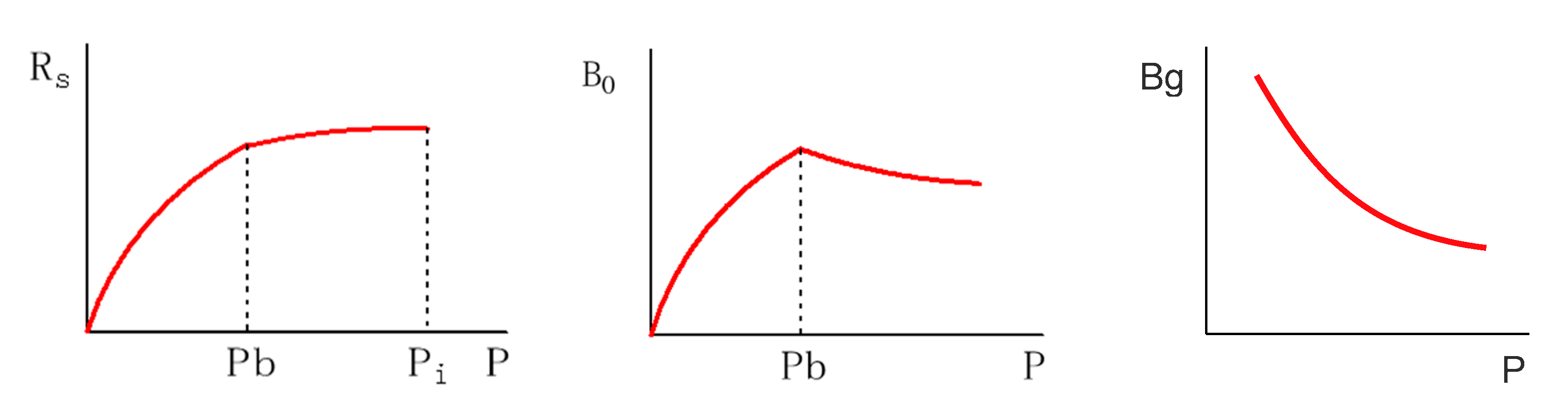
Figure 2.
Schematic diagrams of the relationships between viscosity and pressure of crude oil and natural gas.
Figure 2.
Schematic diagrams of the relationships between viscosity and pressure of crude oil and natural gas.
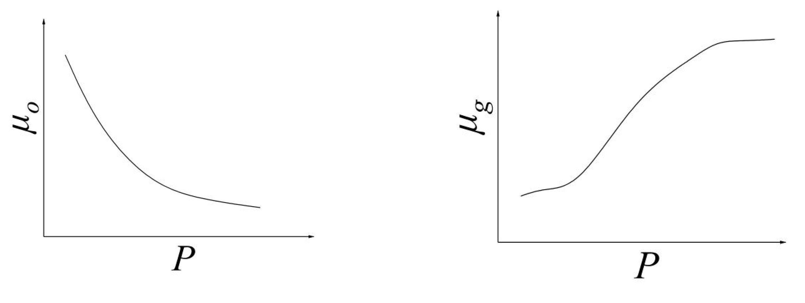
Figure 3.
Schematic diagrams of the relationships between the saturation of formation crude oil, recovery degree and formation pressure.
Figure 3.
Schematic diagrams of the relationships between the saturation of formation crude oil, recovery degree and formation pressure.
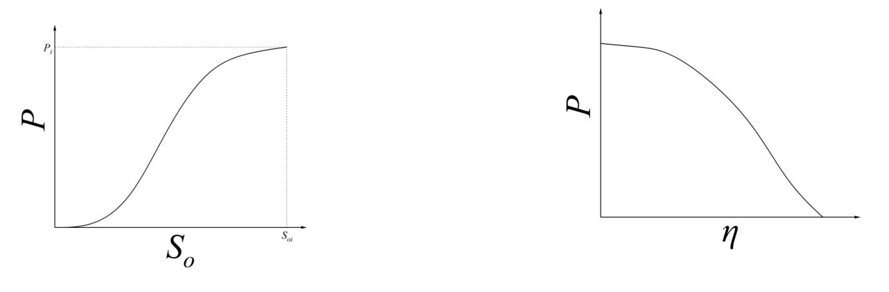
Figure 4.
Schematic diagram of the horizontal well in the upper and lower closed boundary reservoir.
Figure 4.
Schematic diagram of the horizontal well in the upper and lower closed boundary reservoir.
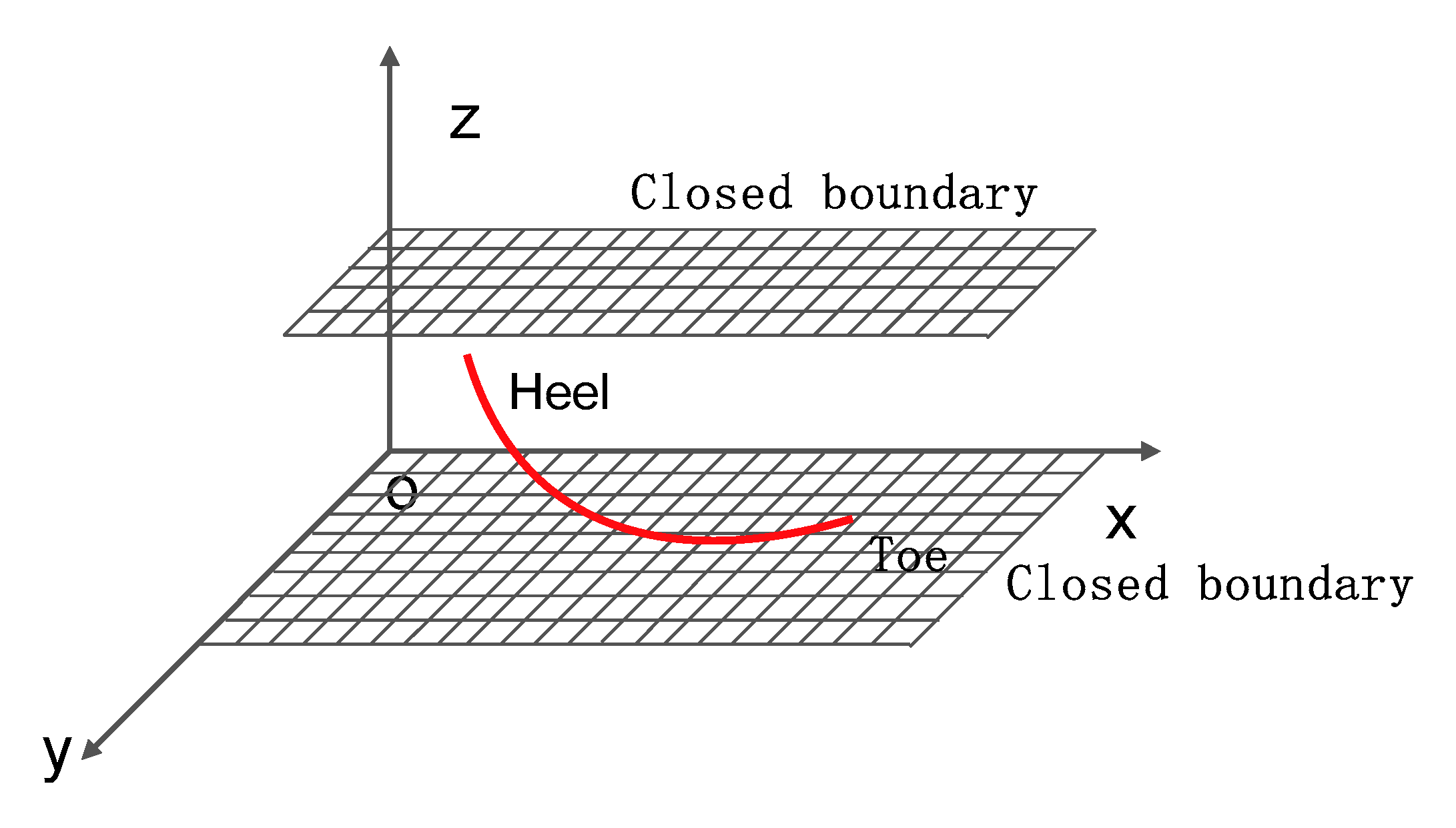
Figure 5.
Mirror of horizontal well in upper and lower enclosed boundary reservoir.
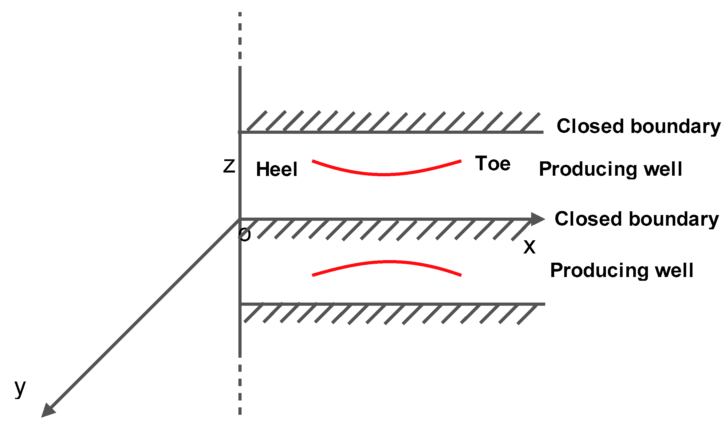
Figure 6.
Oil-gas two-phase seepage curve.
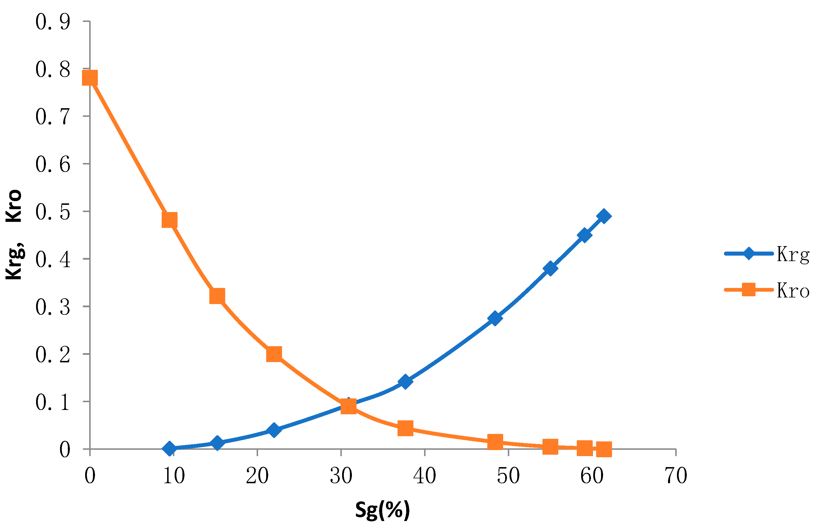
Figure 7.
Formation pressure 30MPa, bottom hole flowing pressure 28MPa, single-phase flow.
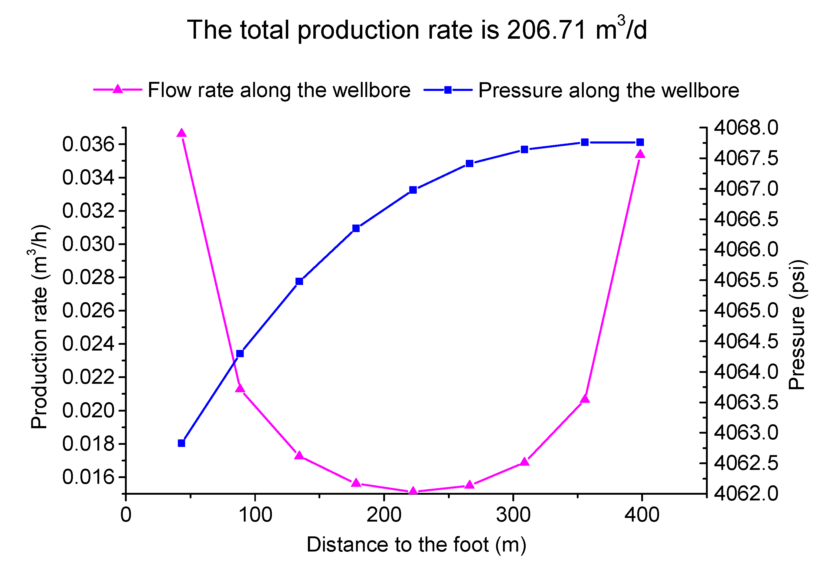
Figure 8.
Formation pressure 18MPa, bottom hole flowing pressure 16MPa, single-phase flow.
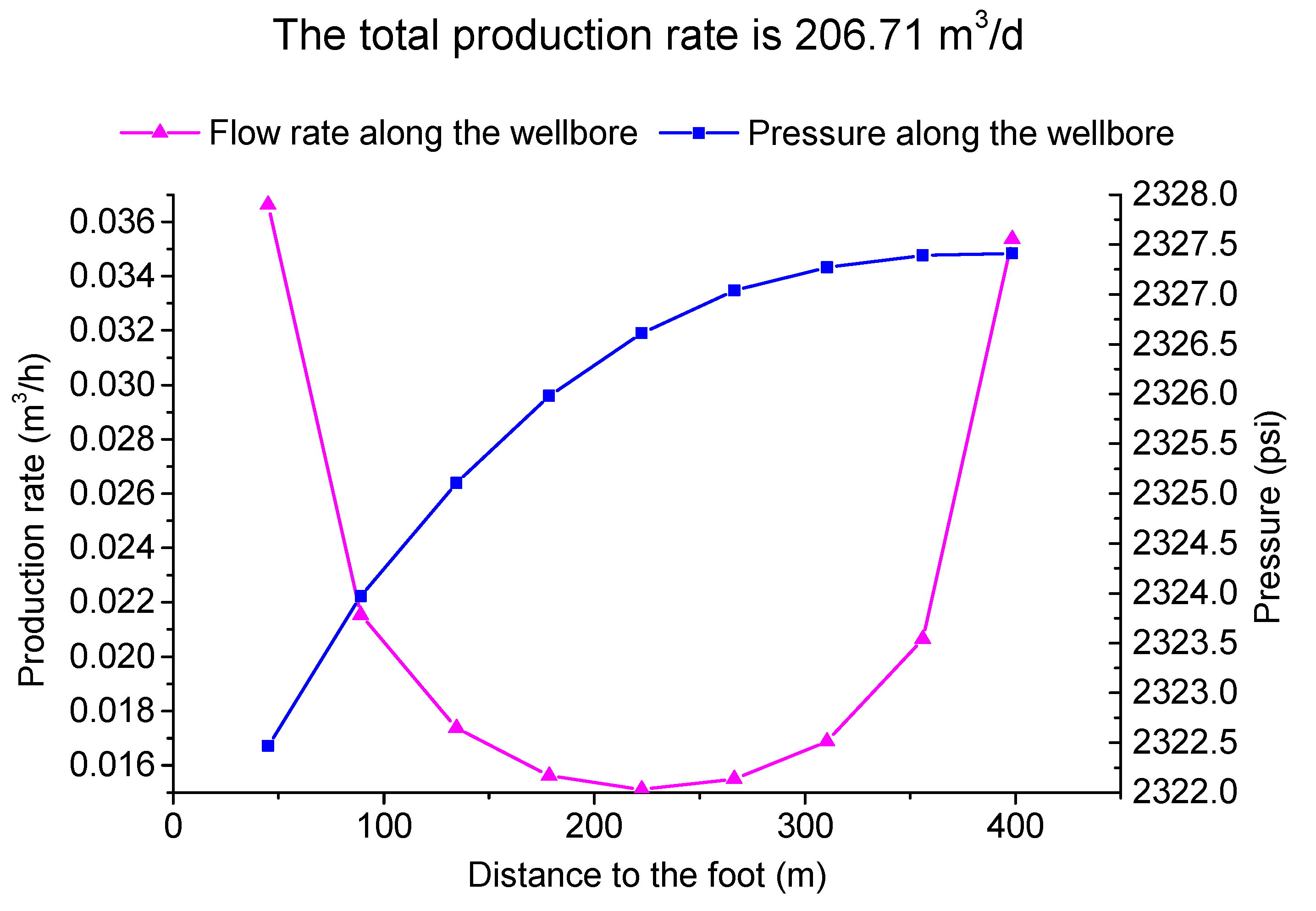
Figure 9.
The formation pressure is 16MPa, the bottom hole flowing pressure is 14MPa, and the oil and gas two-phase seepage occurs.
Figure 9.
The formation pressure is 16MPa, the bottom hole flowing pressure is 14MPa, and the oil and gas two-phase seepage occurs.
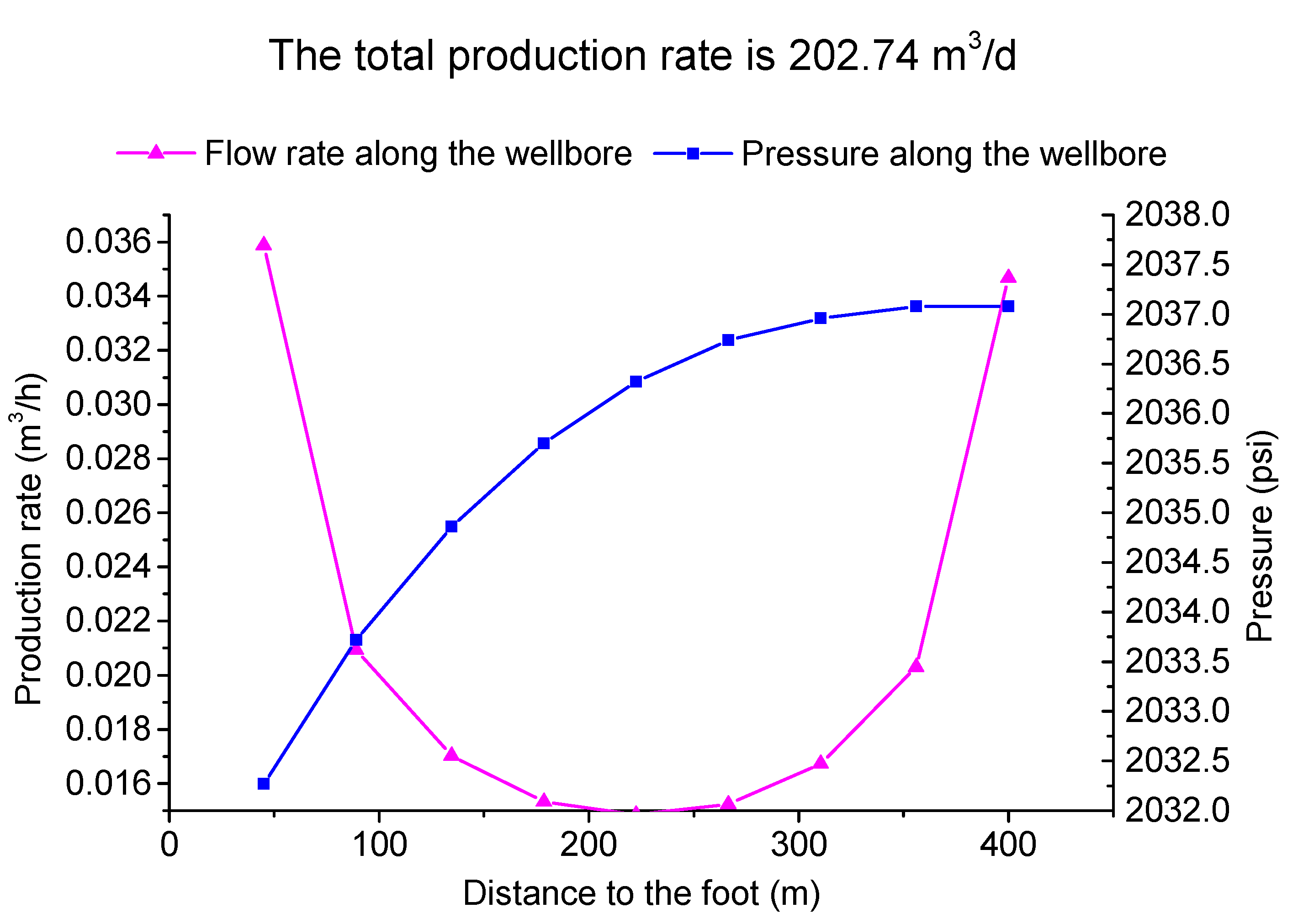
Figure 10.
The formation pressure is 10MPa, the bottom hole flowing pressure is 8MPa, and the degassing is more serious.
Figure 10.
The formation pressure is 10MPa, the bottom hole flowing pressure is 8MPa, and the degassing is more serious.

Figure 11.
Comparison of calculation results and test data of different productivity prediction methods.
Figure 11.
Comparison of calculation results and test data of different productivity prediction methods.
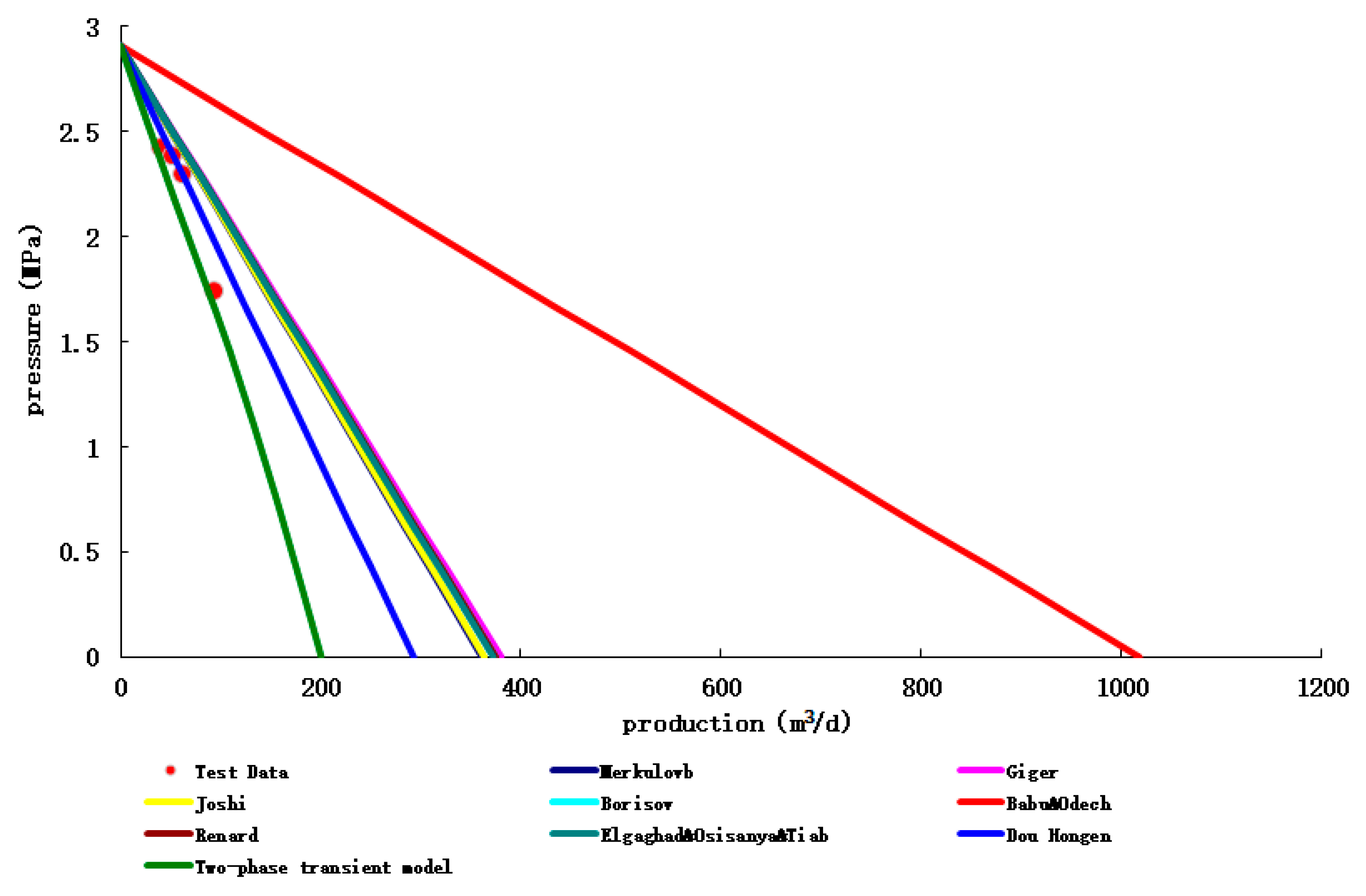
Figure 12.
Comparison of calculation results and test data of different productivity prediction methods.
Figure 12.
Comparison of calculation results and test data of different productivity prediction methods.
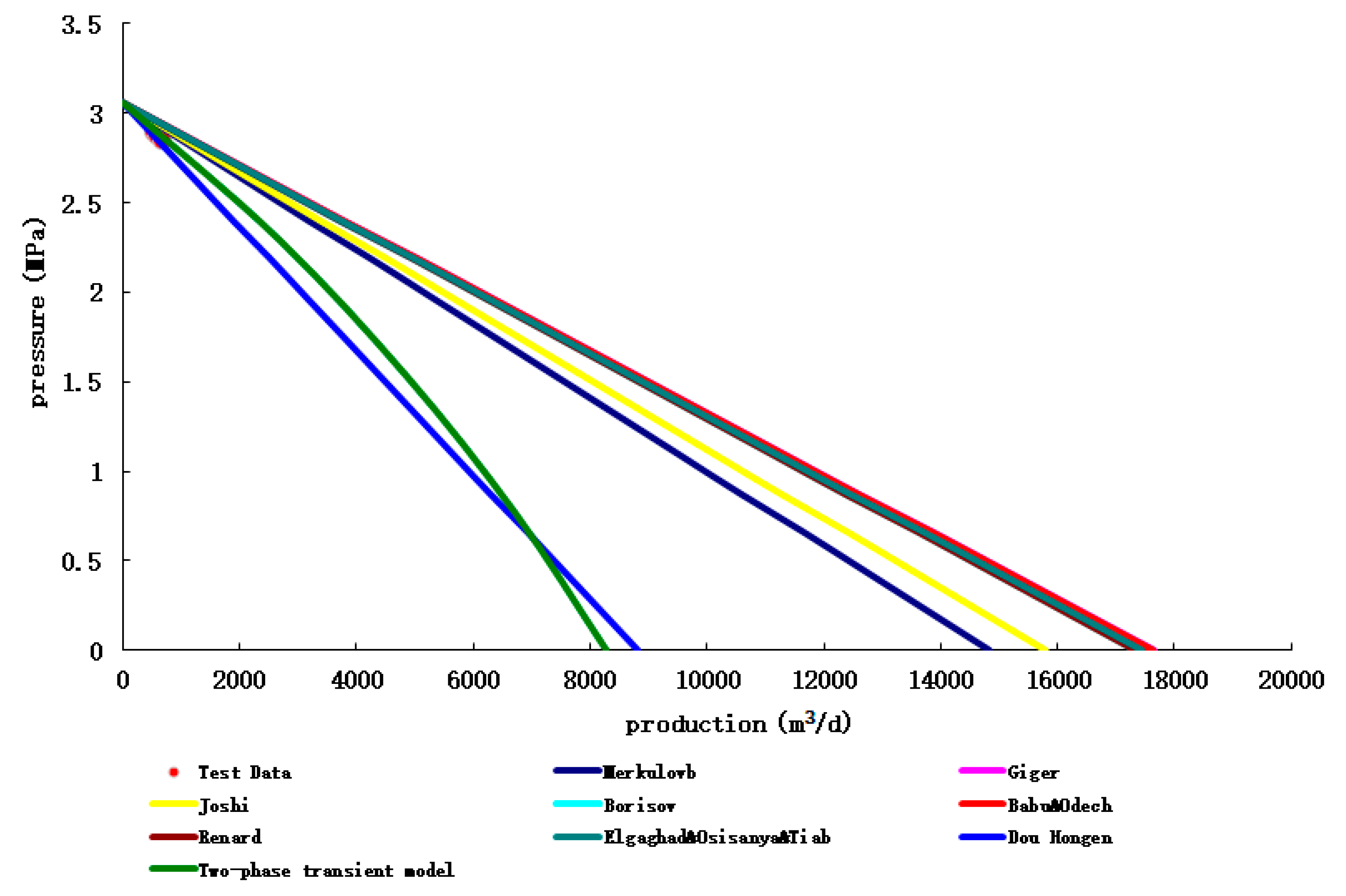
Figure 13.
Comparison of calculation results of different productivity prediction methods with test data.
Figure 13.
Comparison of calculation results of different productivity prediction methods with test data.
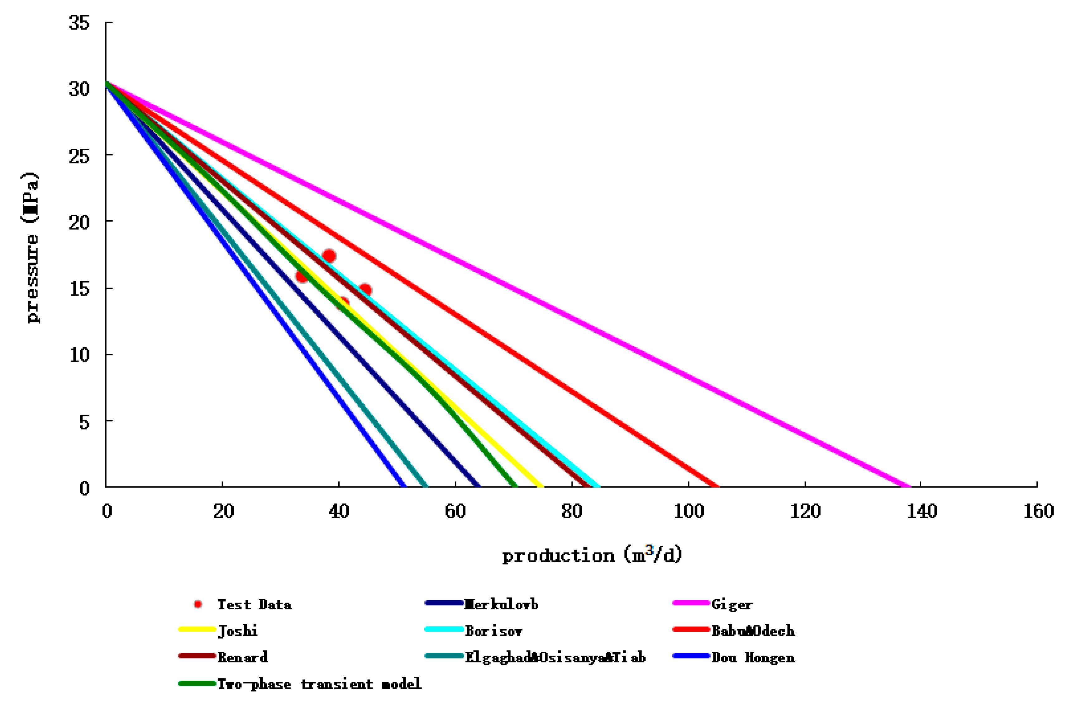
Figure 14.
Comparison of calculation results and test data of different productivity prediction methods.
Figure 14.
Comparison of calculation results and test data of different productivity prediction methods.
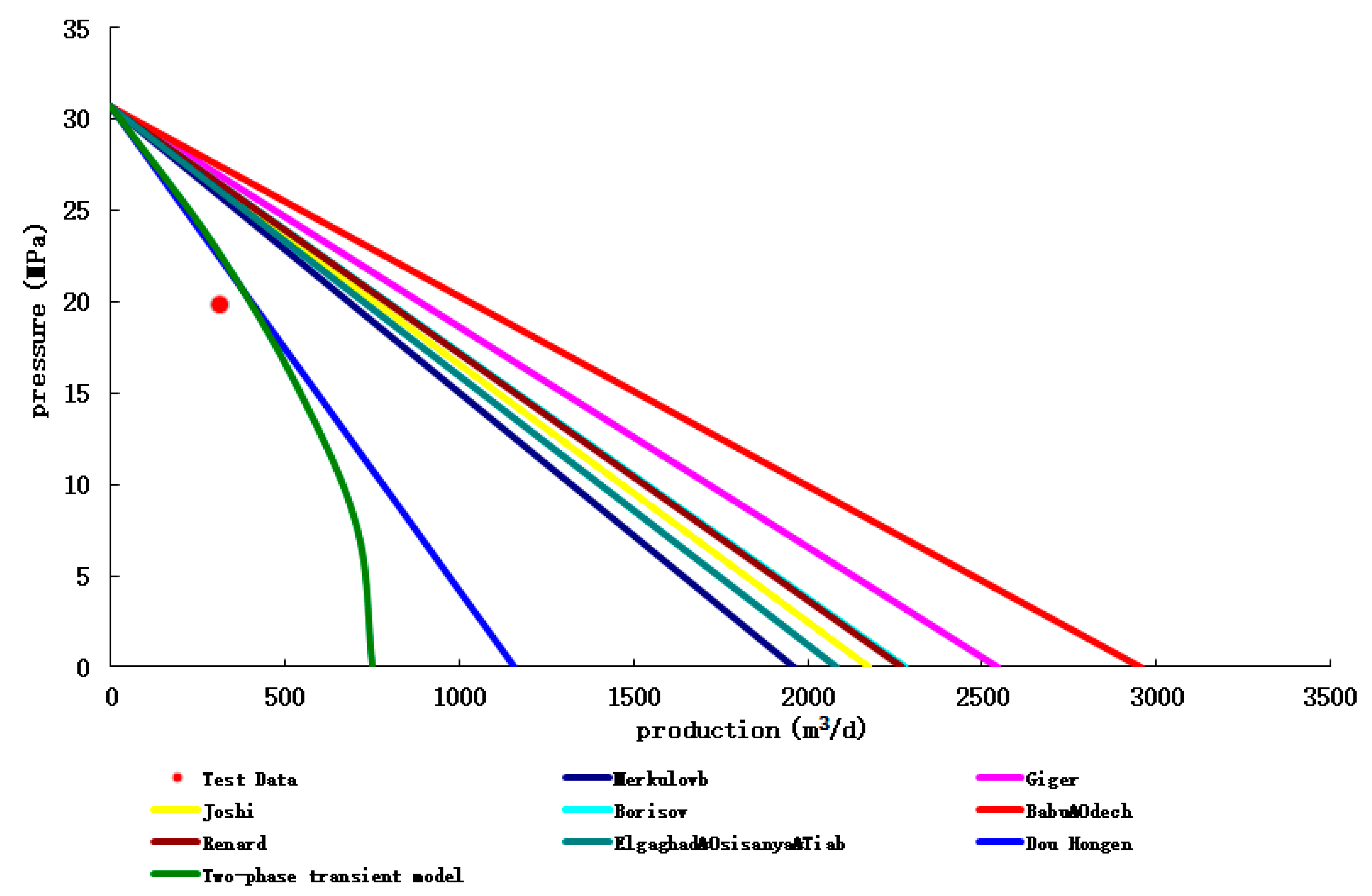
Figure 15.
Comparison of calculation results and test data of different productivity.
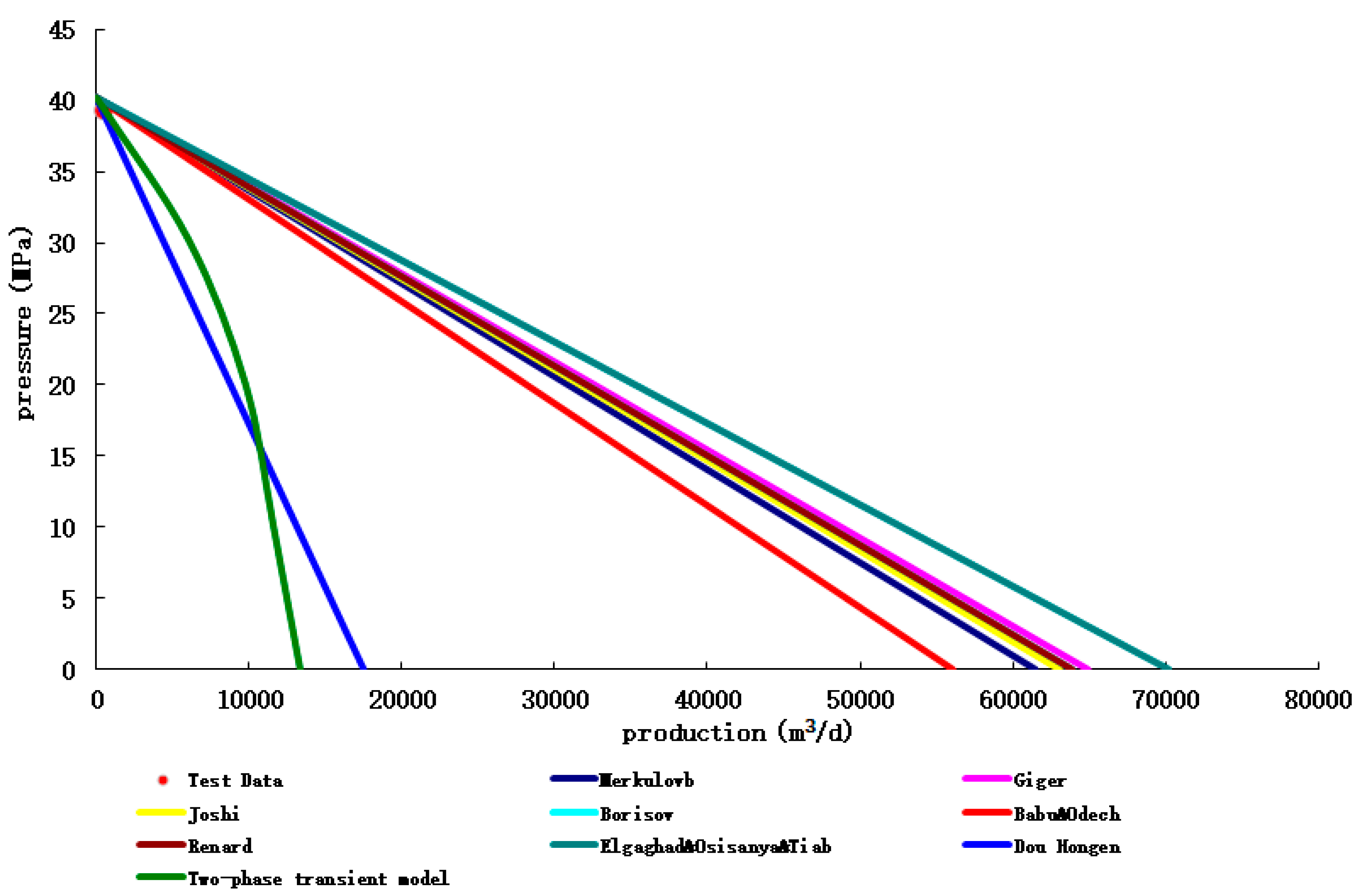

Table 1.
Parameters of oil reservoir and horizontal well.
| name | value | unit |
| Horizontal permeability | 10 | mD |
| Vertical permeability | 10 | mD |
| Crude oil volume factor | 1.281 | |
| porosity | 0.3 | |
| Total compressibility coefficient of formation | 0.0002 | 1/MPa |
| Crude oil viscosity | 0.6365 | mPa.s |
| Reservoir thickness | 30 | m |
| Horizontal well length | 400 | m |
| Original formation pressure | 30 | MPa |
| Well bottom flowing pressure | 28 | MPa |
| Completion method | Open hole completion | |
| Oil reservoir type | The upper and lower closed boundary reservoir | |
| Saturation pressure | 15 | MPa |
| Reservoir temperature | 80 | ℃ |
| Production time | 1 | year |
Table 2.
Reservoir parameters of two horizontal wells.
| Well No. | Oil layer thickness m |
Porosity decimal |
Comprehensive compression factor 1/MPa |
Absolute permeability (in the X, Y direction) mD |
Absolute permeability (in the Z direction mD |
| MIS 320 CN-H7 | 157.79 | 0.116 | 0.001276264 | 43 | 43 |
| MIS 322 C/N-H2 | 157.79 | 0.116 | 0.001276264 | 578 | 578 |
Table 3.
Characteristics of single-phase seepage crude oil in two horizontal wells.
| Well No. | Crude oil volume factor | Crude oil viscosity | Relative density of crude oil |
| MIS 320 CN-H7 | 1.09 | 1.8 | 0.832 |
| MIS 322 C/N-H2 | 1.09 | 1.8 | 0.832 |
Table 4.
Reservoir types and completion parameters of two horizontal wells.
| Well No. | Well type | Reservoir type | Oil drainage area length(x) m |
Oil drainage area length(y) m |
Wellbore length m |
Wellbore diameter in |
skin coefficient in Well Completion | Well reservoir factor (m3/MPa) |
Formation pressure MPa |
| MIS 320 CN-H7 | Horizontal wells | Infinitely large homogeneous reservoirs | 394.1 | 6 1/8” | 10 | 7.093 | 2.91 | ||
| MIS 322 C/N-H2 | 157.79 | Infinitely large homogeneous reservoirs | 1524 | 1524 | 422.34 | 6 1/8” | -3 | 7.093 | 3.059 |
Table 5.
Experimental production data of MIS 320 CN-H7 well.
| No. | Duration | ESP (Hz) | Pwf (psi) | Δp (psi) | Rate(bbl/d) | PI (bbl/d/psi) |
| 1 | 22:00-2:00 | 35 | 351 | 72 | 255 | 3.86 |
| 2 | 2:04-6:15 | 40 | 346 | 77 | 330 | |
| 3 | 6:19-10:15 | 45 | 333 | 90 | 398 | |
| 4 | 10:21-16:00 | 50 | 252 | 171 | 596 |
Table 6.
Experimental production data of MIS 322 CN-H2 well.
| No. | Oil Rate (bbl/d) | ΔP (psi) | Pwf (psi) | Watercut (%) | Choke size (1/64”) | ESP (Hz) | PI (bbl/d/psi) |
| 1 | 3392 | 25 | 419 | 0.2 | 42 | 45 | 136.57 |
| 2 | 3820 | 28 | 416 | 0.2 | 52 | 47 | |
| 3 | 4260 | 31 | 413 | 0.1 | 50 | 50 |
Table 7.
Calculation results of different productivity prediction methods and error analysis of test data.
Table 7.
Calculation results of different productivity prediction methods and error analysis of test data.
| method | Merkulovb | Giger | Joshi | Borisov | Babu&Odech | Renard | Elgaghad | Dou Hongen | Multiphase flow transient model |
| Absolute average relative error (decimal) | 0.369 | 0.442 | 0.378 | 0.422 | 2.859 | 0.422 | 0.413 | 0.120 | 0.096 |
Table 8.
Calculation results of different productivity prediction methods and error analysis of test data.
Table 8.
Calculation results of different productivity prediction methods and error analysis of test data.
| method | Merkulovb | Giger | Joshi | Borisov | Babu&Odech | Renard | Elgaghad | Dou Hongen | Multiphase flow transient model |
| Absolute average relative error (decimal) | 0.519 | 0.808 | 0.617 | 0.775 | 0.806 | 0.775 | 0.787 | 0.097 | 0.103 |
Table 9.
Reservoir parameters of three horizontal wells.
| Well No. | Oil layer thickness m |
Porosity decimal |
Comprehensive compression factor 1/MPa |
Absolute permeability (in the X, Y direction) mD |
Absolute permeability (in the Z direction) mD |
Oil layer temperature ℃ |
| HF003-S001H | 70 | 0.177 | 0.0013154 | 0.076 | 0.02736 | 81.2 |
| HF002-M001H | 30 | 0.115 | 0.001285 | 13.4 | 93.78 | |
| HF001-N002H | 8 | 0.197 | 0.00174 | 861 | 114.27 |
Table 10.
Characteristics of single-phase seepage crude oil in three horizontal wells.
| Well No. | Crude oil volume factor | Crude oil viscosity | Relative density of crude oil |
| HF003-S001H | 1.237 | 1.33 | 0.904 |
| HF002-M001H | 1.55 | 1.643 | 0.794 |
| HF001-N002H | 1.444 | 0.64 | 0.872 |
Table 11.
Reservoir types and completion parameters of three horizontal wells.
| Well No. | Well type | Reservoir type | Wellbore length m |
Wellbore diameter in |
skin coefficient in Well Completion | Well reservoir factor (m3/MPa) |
Formation pressure MPa |
| HF003-S001H | Horizontal wells | Boundary homogeneous reservoirs | 532.1 | 0.15 | -5.69 | 2.49 | 30.38 |
| HF002-M001H | Horizontal wells | Infinitely large homogeneous reservoirs | 579 | 0.15 | -5.47 | 5.99 | 30.659 |
| HF001-N002H | Horizontal wells | 273 | 0.15 | -3.51 | 40.22 |
Table 12.
Experimental production data of HF003-S001H well.
| Date | Time | Choke Size (in) |
WHP (psi) |
Flowing Pressure (psi) |
Differential Pressure (psi) |
Production Rate | |
| Oil (bbl/d) |
Gas ( Mscf/d |
||||||
| 29.8.2011 | 14:53 | 16/64 “ | / | 2522.46 | 1760.4 | 241.6 | 161.2 |
| 30.8.2011 | 2:23 | 20/64 “ | / | 2141.11 | 2141.75 | 280.6 | 167.1 |
| 30.8.2011 | 10:42 | 24/64 “ | / | 1990.89 | 2291.97 | 255.6 | 221.8 |
| 30.8.2011 | 16:23 | 16/64 “ | / | 2301.37 | 1981.49 | 213.5 | 109.7 |
Table 13.
Experimental production data of HF002-M001H well.
| Choke Size (in) |
WHP (psia) |
Flowing Pressure (psia) |
Differential Pressure (psi) |
Production Rate | ||
| Fluid (bbl/d) |
Oil (bbl/d) |
GOR (scf/bbl) |
||||
| 48/64 | 450 | 2870.405 | 1454.19 | 1992 | 1992 | 976 |
Table 14.
Experimental production data of HF001-N002H well.
| Oil Production Rate (bbl/d) | Flowing Pressure (psi) |
| 3263.6 | 5693.99 |
Table 15.
Calculation results of different productivity prediction methods and error analysis of test data.
Table 15.
Calculation results of different productivity prediction methods and error analysis of test data.
| method | Merkulovb | Giger | Joshi | Borisov | Babu&Odech | Renard | Elgaghad | Dou Hongen | Multiphase flow transient model |
| Absolute average relative error (decimal) | 0.196 | 0.731 | 0.092 | 0.104 | 0.318 | 0.102 | 0.309 | 0.356 | 0.098 |
Table 16.
Calculation results of different productivity prediction methods and error analysis of test data.
Table 16.
Calculation results of different productivity prediction methods and error analysis of test data.
| method | Merkulovb | Giger | Joshi | Borisov | Babu&Odech | Renard | Elgaghad | Dou Hongen | Multiphase flow transient model |
| Absolute average relative error (decimal) | 1.195 | 1.849 | 1.436 | 1.552 | 2.308 | 1.542 | 1.332 | 0.297 | 0.257 |
Table 17.
Calculation results of different productivity prediction methods and error analysis of test data.
Table 17.
Calculation results of different productivity prediction methods and error analysis of test data.
| method | Merkulovb | Giger | Joshi | Borisov | Babu&Odech | Renard | Elgaghad | Dou Hongen | Multiphase flow transient model |
| Absolute average relative error (decimal) | 1.829 | 1.987 | 1.901 | 1.940 | 1.580 | 1.940 | 2.230 | 0.194 | 0.116 |
Table 18.
Total average error statistics of 5 wells.
| Forecasting methodology | Merkulovb | Giger | Joshi | Borisov | Babu&Odech | Renard | Elgaghad | Dou Hongen | Multiphase flow transient model |
| MIS 320 CN-H7 | 0.369 | 0.442 | 0.378 | 0.422 | 2.859 | 0.422 | 0.413 | 0.12 | 0.096 |
| MIS 322 CN-H2 | 0.519 | 0.808 | 0.617 | 0.775 | 0.806 | 0.775 | 0.787 | 0.097 | 0.103 |
| HF003-S001H | 0.196 | 0.731 | 0.092 | 0.104 | 0.318 | 0.102 | 0.309 | 0.356 | 0.098 |
| HF002-M001H | 1.195 | 1.849 | 1.436 | 1.552 | 2.308 | 1.542 | 1.332 | 0.297 | 0.257 |
| HF001-N002H | 1.829 | 1.987 | 1.901 | 1.94 | 1.58 | 1.94 | 2.23 | 0.194 | 0.116 |
| Average error | 0.8216 | 1.1634 | 0.8848 | 0.9586 | 1.5742 | 0.9562 | 1.0142 | 0.2128 | 0.134 |
Disclaimer/Publisher’s Note: The statements, opinions and data contained in all publications are solely those of the individual author(s) and contributor(s) and not of MDPI and/or the editor(s). MDPI and/or the editor(s) disclaim responsibility for any injury to people or property resulting from any ideas, methods, instructions or products referred to in the content. |
© 2023 by the authors. Licensee MDPI, Basel, Switzerland. This article is an open access article distributed under the terms and conditions of the Creative Commons Attribution (CC BY) license (http://creativecommons.org/licenses/by/4.0/).
Copyright: This open access article is published under a Creative Commons CC BY 4.0 license, which permit the free download, distribution, and reuse, provided that the author and preprint are cited in any reuse.


