Preprint
Essay

Machine Learning-Based Classification of Digital Media Traffic

Altmetrics

Downloads

169

Views

59

Comments

0

Submitted:

18 April 2023

Posted:

18 April 2023

You are already at the latest version

Alerts
Abstract
The exponential growth of digital media content has introduced new challenges in managing and classifying internet traffic. Digital media traffic is composed of various applications such as video, audio, social media, and search, and its data structure is complex, incorporating a vast array of features. The classification of traffic data is a crucial aspect of internet traffic management and network security, and it forms the basis for several scenarios, including content distribution, advertising recommendations, and data analysis. Traditional classification methods rely mainly on deep packet inspection and port-based techniques, which have become increasingly ineffective due to the rapid evolution of network traffic. To address this issue, this study proposes a machine learning-based traffic classification method aimed at enhancing the accuracy and efficiency of digital media traffic classification to meet the current needs of traffic management and network security. The paper also analyzes and evaluates the classification effect and prediction capability of various algorithms under different training set sizes to validate the feasibility and effectiveness of the proposed method. The result demonstrates that the neural network algorithm has superior classification and prediction capabilities compared to the decision tree and support vector machine algorithms. Furthermore, our proposed method achieves the highest accuracy of 96.88% with a large training sample of 40,000 data streams, proving its superiority in handling high-dimensional data and complex datasets. The research results are significant for the development of digital media traffic classification and prediction methods and are expected to be applied in practical scenarios.
Keywords: 
Subject: Computer Science and Mathematics  -   Mathematics

1. Introduction

The continuous development and increasing popularity of digital media technology has made it an integral part of people's lives. Digital media takes many forms including text, images, audio and video, and the volume of traffic transmitted over the network is constantly growing. However, the rapid growth of digital media has led to a number of challenges, including digital media traffic management. This involves managing and optimizing the transmission of digital media in the network [1]. Digital media traffic classification is a crucial technique in digital media traffic management. It helps network administrators understand network usage and develop better network strategies. Moreover, digital media traffic classification assists network security personnel in identifying malicious traffic and network attacks. Therefore, digital media traffic classification is of great practical significance and has broad application prospects [2,3].
Currently, several approaches are used to classify digital media traffic, including port number and protocol-based approaches, traffic feature-based approaches, and deep learning-based approaches [4,5]. Nguyen et al. [3] reviewed the current state of research on Internet traffic classification and obfuscation techniques, analyzed the limitations of traditional classification methods in terms of complex management and handling of new traffic features, and summarized various data representation methods and the different objectives of Internet traffic classification. Currently, the traffic feature-based approach has become one of the mainstream methods for classifying digital media traffic. This approach uses statistical features in traffic, such as packet size, time interval, and transmission rate, to categorize traffic. Clustering algorithms, such as K-means and KNN, and classification algorithms, such as SVM, are widely used to classify digital media traffic. Erman et al. [6] used an unsupervised K-means algorithm to identify core traffic (e.g. P2P, Web, TFP, etc.) using average message interval, stream duration, average message length, etc. as specialization values. William et al. [7] compared five machine learning algorithms: discrete plain Bayesian, plain Bayesian kernel, C4.5 decision tree, Bayesian network, and Bayesian tree. The experimental results show that all four algorithms can achieve 90% classification accuracy except for the plain Bayesian kernel, but the computational performance of each algorithm varies greatly, with C4.5 being the fastest. However, these methods have several practical limitations. Firstly, manual feature extraction is often required, and feature selection often requires significant domain knowledge and experience. Secondly, these methods often do not handle encrypted traffic or multi-purpose traffic well, and the computational complexity is often high. Finally, these methods are less efficient when dealing with large-scale traffic data. To address the limitations of traditional classification methods, researchers have developed deep learning-based methods, such as convolutional neural networks and recurrent neural networks, for classifying digital media traffic. These methods use end-to-end learning and classification algorithms, avoiding the problem of manual feature extraction, and achieve higher accuracy and stronger generalisation capabilities than traditional methods. For example, Zhang et al. [8] used deep convolutional neural networks for end-to-end learning and classification of traffic, achieving high classification accuracy and strong generalisation capability in experiments. Similarly, Bryan et al. [9] proposed an SDN-based method for classifying digital media traffic, which achieved high classification accuracy and fast classification speed in experiments. Wang et al. [10] compared the classification performance of 1-dimensional and 2-dimensional CNNs with the traditional classification algorithm C4.5 algorithm. Wu et al. [11] compared theoretically and experimentally the advantages of 2D CNNs over 1D networks, traditional machine learning algorithms, and RNN networks in terms of computation and number of parameters, respectively, without inferior performance to the control group. Although deep learning methods have shown promising results, they have some limitations in the field of digital media traffic classification [12]. Firstly, they require a large amount of training data to improve their accuracy and generalisation ability. However, data collection and annotation are difficult in this field, limiting the amount of available training data. Secondly, feature extraction is challenging because different types of digital media have different features and structures, requiring different feature extraction methods. Finally, deep learning methods require significant time and computational resources for model training, which can increase the difficulty and cost of implementing the algorithm.
This study investigates the suitability, advantages, and limitations of different algorithms for digital media traffic classification. Three classical machine learning algorithms, decision trees, support vector machines, and neural networks, were compared in terms of their performance. The experimental results demonstrate that all three algorithms can solve the digital media traffic classification problem, but their performance and applicability vary. Decision trees and support vector machines exhibit better performance when the data volume is small and the feature dimension is low, whereas neural networks exhibit better classification performance when the data volume is large and the feature dimension is high. Therefore, this study provides valuable insights for using machine learning techniques to address digital media traffic classification problems.

2. Materials and Methods

2.1. Subsection

The decision tree is a classification and regression model that uses a tree-like graph structure and is an intuitive, easy to understand and explain machine learning algorithm [13,14]. This algorithm works by continuously dividing a dataset into smaller subsets through the selection of features, generating a tree that can be used to classify or regress new data for prediction. The decision tree algorithm consists of three main steps: feature selection, tree generation, and pruning. Figure 1 presents a schematic diagram and the primary algorithms of decision trees. Several decision tree algorithms are available, including the ID3 algorithm, which is one of the earliest proposed decision tree algorithms that uses the information gain metric to select optimal features for splitting. The C4.5 algorithm is an improved version of the ID3 algorithm that uses the information gain rate metric to avoid the bias problem of ID3 algorithm. Additionally, C4.5 supports the processing of missing and continuous value features [15,16]. The CART algorithm, another decision tree algorithm, can be used for classification and regression, using the Gini index to select the optimal features for splitting. Unlike the ID3 and C4.5 algorithms, the CART algorithm generates a binary tree with only two branches per node. This paper uses the CART algorithm for the classification of digital media traffic.

2.2. Support vector machine

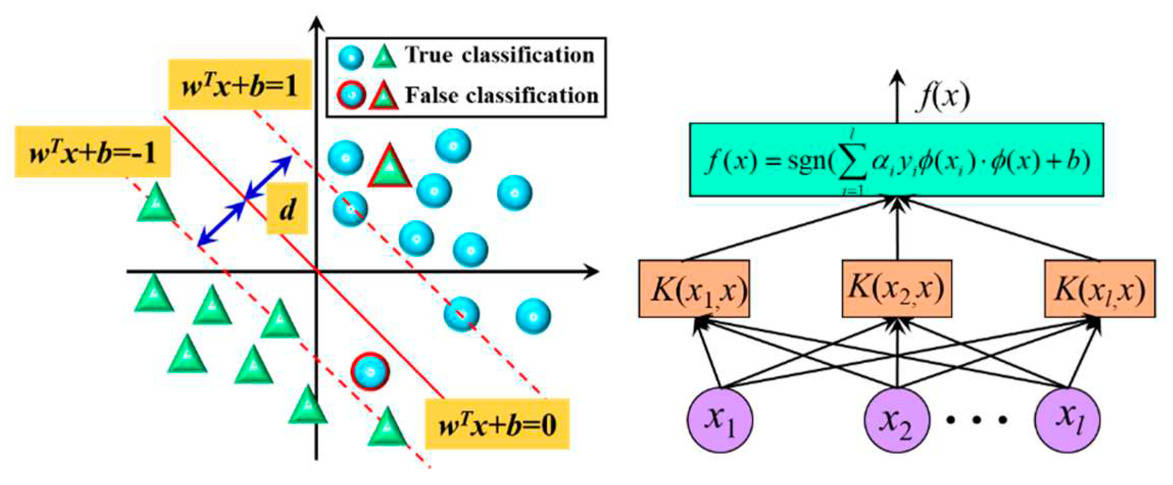
Support Vector Machine (SVM) is a machine learning algorithm based on the theory of VC dimensionality in statistical learning and the principle of structural risk minimisation [17,18]. SVM aims to construct an optimal decision function based on the maximum margin principle that can classify test data correctly by learning from training samples. Specifically, SVM finds the hyperplane with the maximum margin between the two categories based on the distances between the samples in the two categories. This hyperplane can be represented by the equation wTx+ b =0, where w is the normal vector of the hyperplane and b is the offset of the hyperplane [19]. Figure 2 illustrates the concept of SVM, where the blue circle represents category 1, the green triangle represents category 2, the two red dashed lines indicate the boundaries of categories 1 and 2, which are called support vectors, and the red solid line in the middle of the support vectors indicates the optimal hyperplane.
Based on the idea of maximum interval theory, the SVM model can be described by equation (1), which is able to describe a typical convex quadratic programming problem with linear constraints by determining its maximum interval classification hyperplane, and the Lagrangian function can be described by equation (2).
min w w 2 / 2 s . t . y i ( < w , x i > + b ) 1 ,
L ( w , b , α ) = 1 2 w 2 i = 1 m α i ( y i < w , x i + b > 1 ) ,

2.3. BP neural network

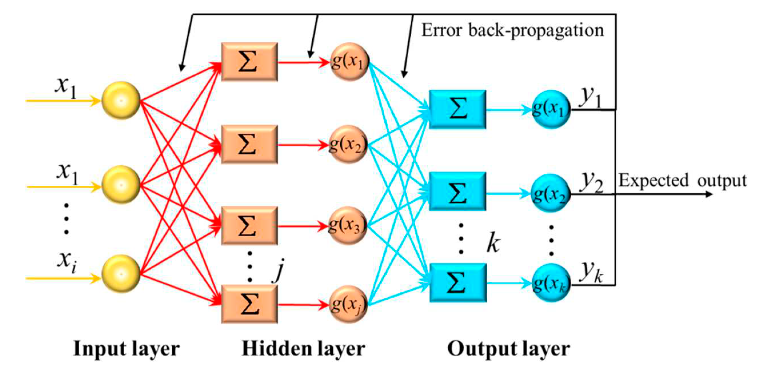
BP network is a feedback-free forward network, the neurons in the network are arranged in layers, the output of the neurons within each layer are transmitted to the next layer, this transmission by the right of coupling to achieve the output [20]. The work process is divided into two parts: the learning period and the working period. The key to the calculation lies in the back-propagation process of the error in the learning period, which minimizes the objective function to complete the process, and the structure of its completion process is shown in Figure 3 below:
As shown in Figure 3, the neurons in the input, hidden and output layers are numbered with The inputs of each neuron in the implicit and output layers are:
n e t j = i w j i o i ,
n e t k = j w k j o j ,
The outputs of the individual neurons in the implicit and output layers are:
o j = g ( n e t j ) ,
o k = g ( n e t k ) ,
where the activation functions are all unipolar functions [21], i.e:
g ( x ) = 1 1 + e x ,
When the output of the network o k is not equal to the actual output y k (expected value), there is a training error, and the average error of the system is:
e = 1 2 ( o k y k ) 2 ,
The total error of the network is expressed as:
E = 1 2 k ( o k y k ) 2 ,
The above equation (9) is the objective function of the BP neural network, and the back-propagation of the error during the learning period is accomplished by minimising the objective function.
The adjustment of the weights of each layer is a reverse process, i.e. the weights w k j between the implied layer and the output layer are adjusted by the error signal δ k obtained by comparing the actual output value y k with the actual one.
δ k = ( y k o k ) o k ( 1 o k ) ,
w k j ( n ) = w k j ( n 1 ) + η δ k o j + α Δ w k j ( n 1 ) ,
The error signal δ k is then passed backwards to the input layer to obtain the input layer error signal δ j , which serves to adjust the weights between the input layer and the implied layer.
δ j = o j ( 1 o j ) k δ k w k j ,
w j i ( n ) = w j i ( n 1 ) + η δ j x i + α Δ w j i ( n 1 ) ,
The learning rate, denoted by η , and the momentum term, denoted by α , are used to accelerate the training process of the backpropagation (BP) neural network and to maintain its stability. After training the network and meeting the desired requirements, the interconnection weights between the nodes are fully determined, and the entire BP network is considered trained.

3. Model development

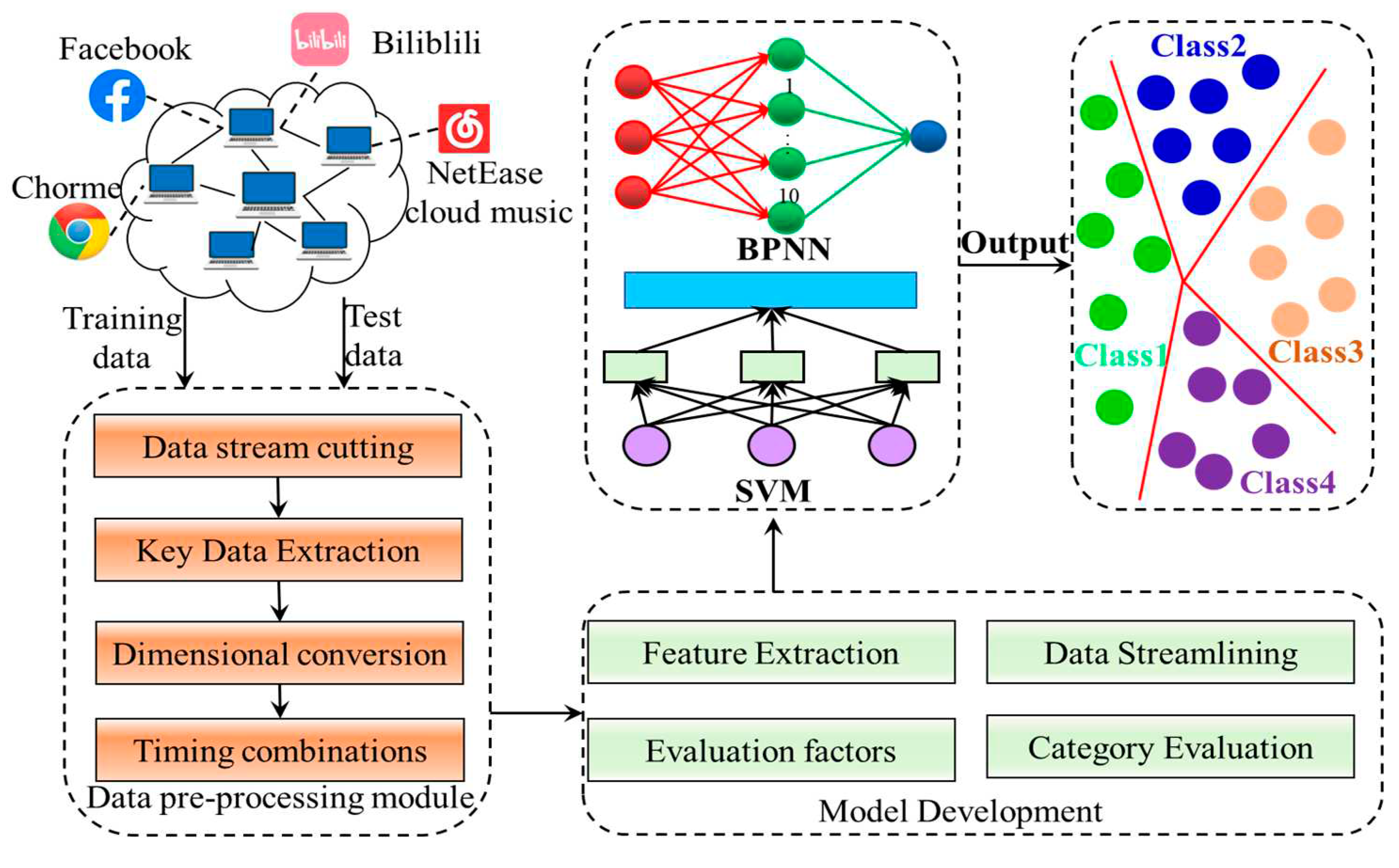
The network traffic classification system based on machine learning comprises four main modules: data acquisition, data pre-processing, model building, and testing. The data acquisition module collects data in the form of text, video, and audio. The data pre-processing module comprises four parts: data stream segmentation, key feature extraction, dimensional conversion, and temporal combination. A series of components and strategies are employed during the machine learning training process to streamline the number of parameters, control the data size during training, categorize the data based on existing knowledge, and calculate the feedback amount by comparing the results with the labels for updating network parameters. The trained network model can be evaluated promptly. Figure 4 illustrates the specific steps of the system.

3.1. Dataset acquisition

In the experiments, we chose a subset of data from various network applications collected in a specific region. During the traffic collection process, communication data generated by different applications coexists in the network as the communication process of the applications is discontinuous. The process manager is used to obtain the port number currently occupied by the application using the correspondence between host ports and applications, and the port filtering function is used to collect the communication data of four different applications [22], including Facebook, Chrome, Bilibili, and NetEase Cloud Music, corresponding to four common application types: chat, browser, video, and audio. We parsed the feature extraction using the method described above and parsed it into sample streams. The sample streams contained the largest number of Facebooks, accounting for over 30% of the data. To ensure fairness among different types of streams and the efficiency of the machine learning algorithm, we reduced the number of traffic types that accounted for a significant proportion and kept the experimental data set between 10,000 and 50,000 stream samples. The experiments were conducted on a laboratory PC computer, and the algorithm implementation language was Python. The three machine learning algorithms proposed in this paper were used to train 20,000 samples, and 200 samples were feature classified based on the training results, as shown in Table 1, to compare and study the training effect and classification accuracy of different algorithms. We also explored the effect of the number of training samples on the classification accuracy of different algorithms by selecting 20,000, 30,000 and 40,000 samples for training and classifying 2,000 samples based on their features.

3.2. Data pre-processing module

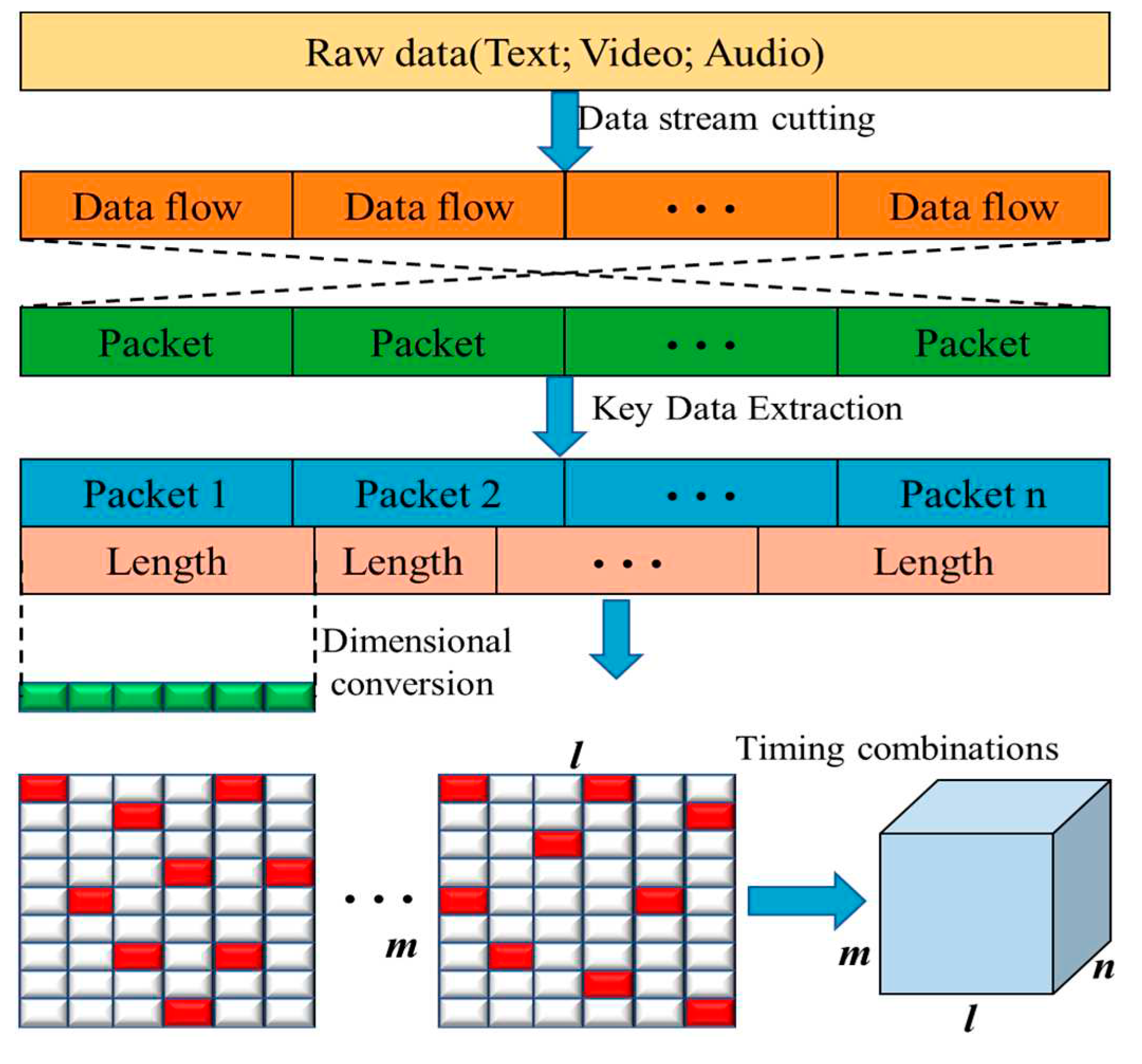
The pre-processing of data in the system is performed in four phases as shown in Figure 5. The first phase is data stream cutting, followed by key data extraction, dimensional transformation, and temporal combination.
The purpose of the data stream cutting process is to segment the original network traffic into individual streams, with each stream serving as a sample. These streams are distinguished by packets with identical source IP addresses, source port numbers, destination IP addresses, destination port numbers, and transport layer protocols. In the key data extraction step, the initial n packets of each stream are extracted and any subsequent packets are discarded, and if the stream is too short, it is padded with zeros [23]. The IP address and MAC address of the data link layer are removed by anonymization, as they may affect the feature extraction process if different flows originate from different networks. The pre-processing module converts the input traffic data into a suitable format for machine learning models. The first step is stream slicing, which divides the original traffic into discrete units by using packets with identical five components. The next step is key data extraction, which involves taking the first n packets of each stream and discarding any packets that exceed them. The anonymisation process then removes the IP and MAC addresses to avoid affecting feature extraction. To standardize the packet length, the first l bytes of data are extracted, and any data exceeding that length is discarded. The remaining data is then one-hot encoded with m bits for each byte, resulting in l ×m 2D data. Next, the data is combined in sequence, and the two-dimensional data corresponding to n data packets are combined into three-dimensional data of l ×m×n. This process is analogous to creating a video file by combining multiple image frames. The resulting data is suitable for input to machine learning models.

3.3. Model evaluation indicators

Accuracy and recall reflect two different aspects of classification quality, which must be considered together and not in isolation, so an assessment indicator that takes both into account is also used. As such, another indicator F1-score is used to evaluate the performance of the model when the data sets are unbalanced. F1-score is expressed as:
F 1 = 2 × P p r e × P r e c P p r e + P r e c ,
The range of F1 is between 0 and 1. Ppre and Prec are the precision and recall of the proposed method. Ppre is expressed as:
P p r e = T P T P + F P ,
The recall Prec is defined as:
P r e c = T P T P + F N

4. Experiments and results

4.1. Results of the decision tree algorithm

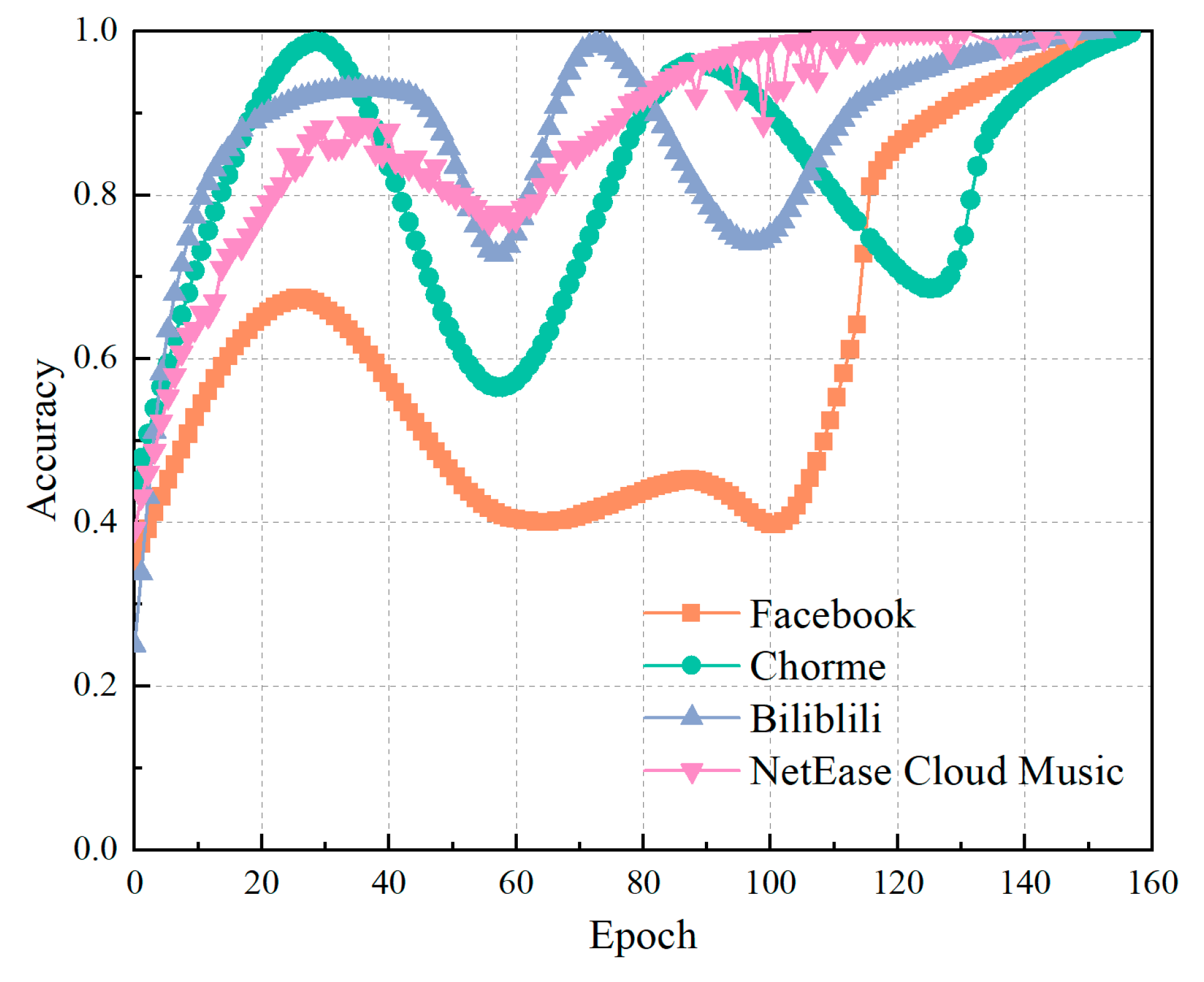
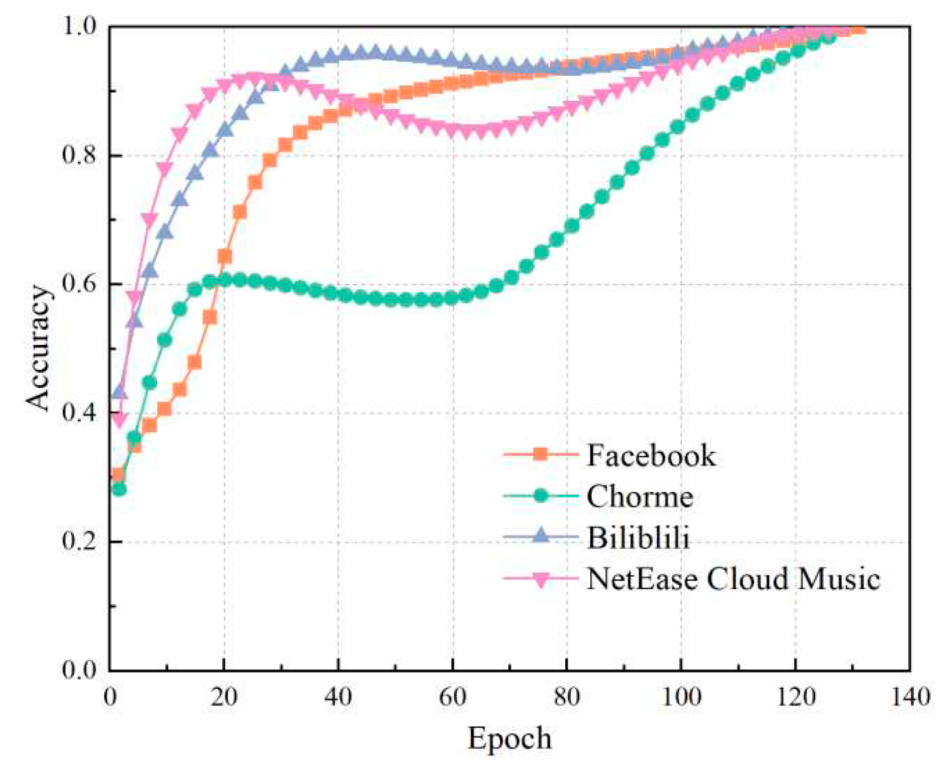
The established decision tree algorithm model was utilized for training, and the recursive partitioning process was halted when all samples within a given node belonged to the same class. Majority voting was used when there were no attributes left to further divide the samples. At this point, the given node was converted into a leaf and labeled with the class where the majority of the samples belonged. Figure 6 displays the convergence of the accuracy of the decision tree training process for classifying sample traffic.
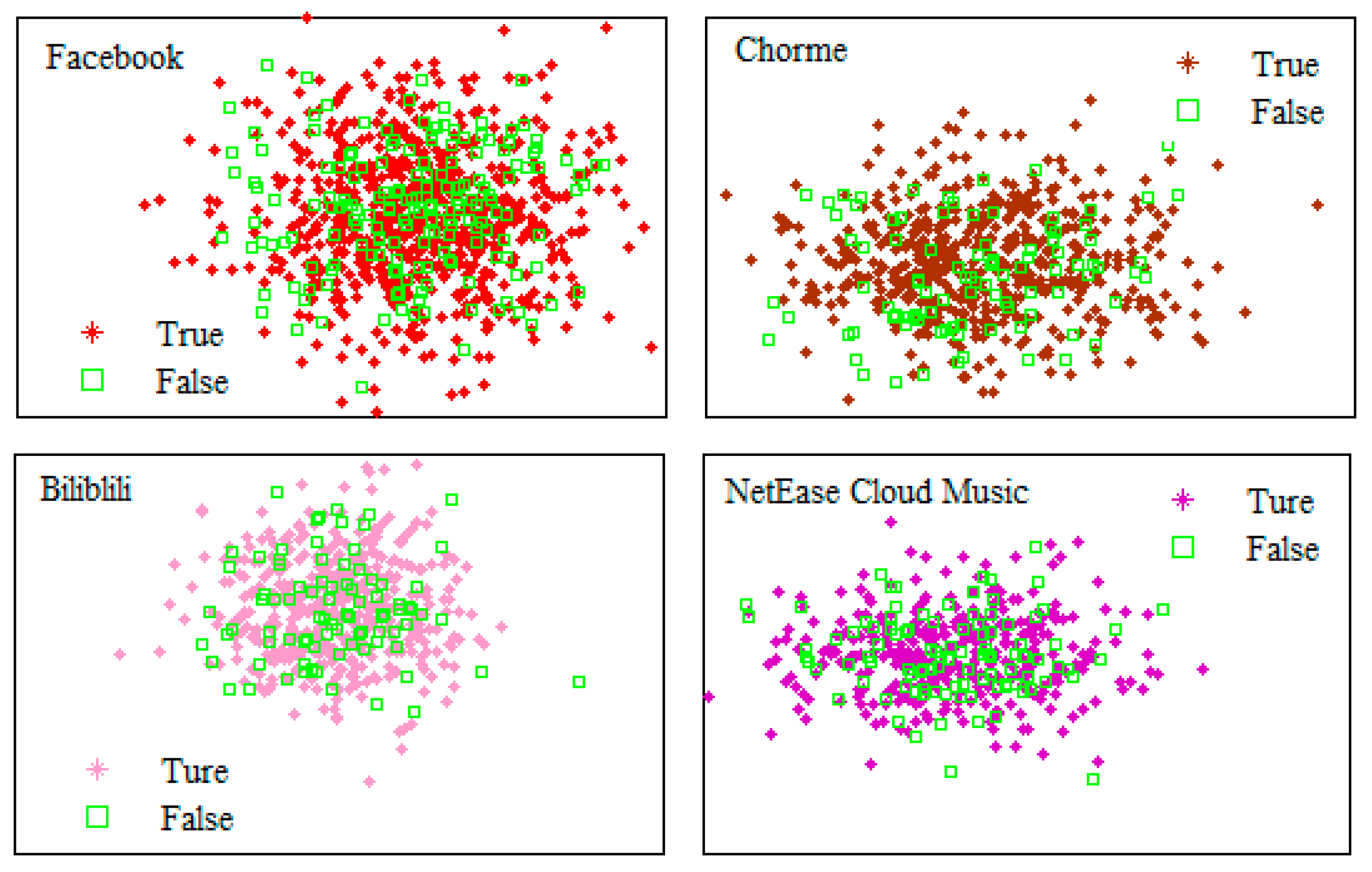
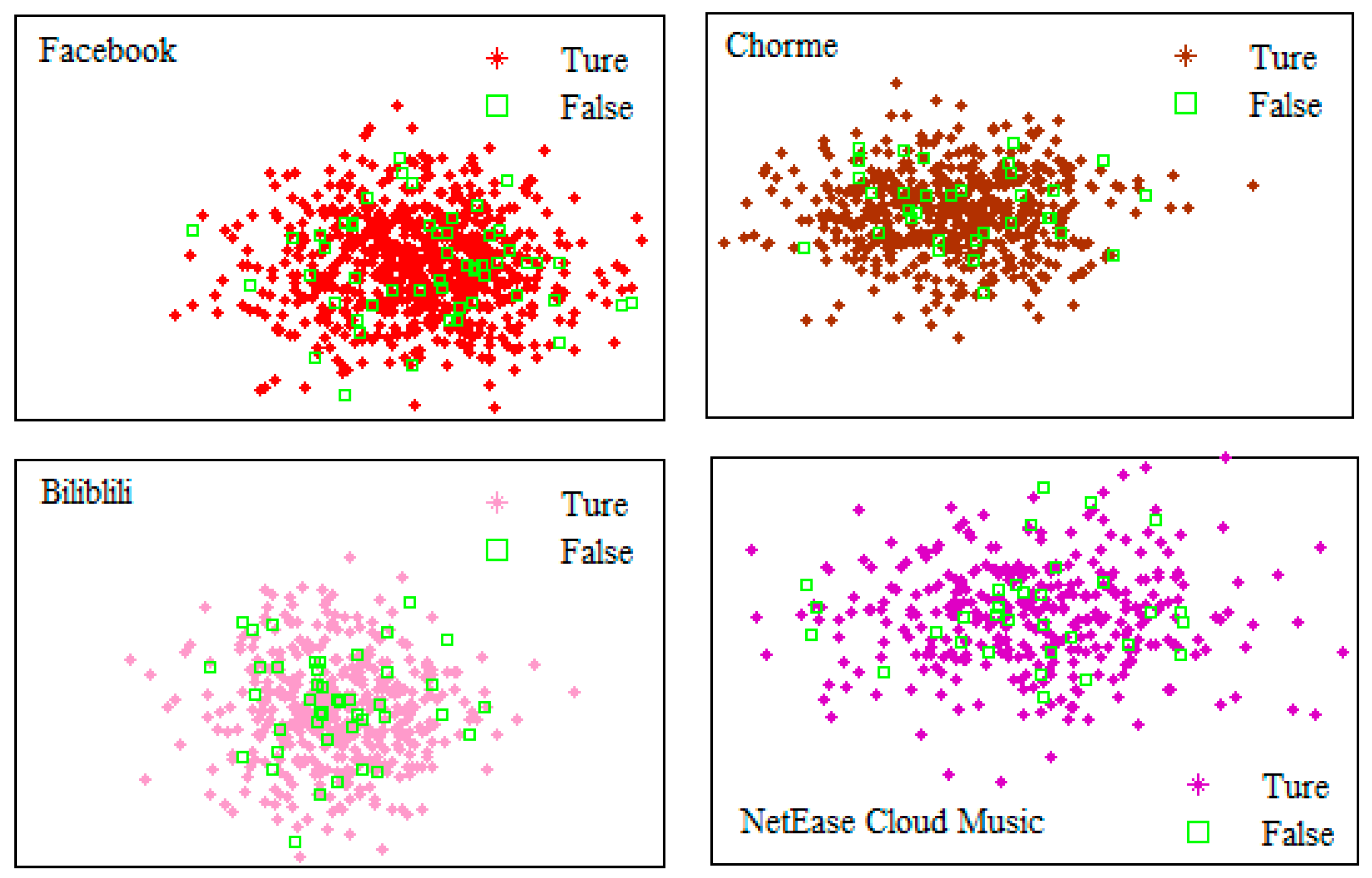
It can be seen from Figure 6, the decision tree algorithm stopped training after 158 iterations. The classification accuracy for the four application types increased from 25% during training and then experienced significant fluctuations before reaching clear classification rules. These fluctuations may have occurred because the decision tree algorithm was insensitive to missing values, resulting in training errors. Figure 7 illustrates the classification of test samples.
The decision tree algorithm achieved accuracy rates of 74.00%, 81.21%, 80.23%, and 69.71% for the Facebook, Chrome, Bilibili, and NetEase Cloud Music applications, respectively, resulting in an overall accuracy of 76.50%. However, as shown in Figure 7, the decision tree algorithm displayed significant errors in overall classification, with uneven accuracy rates across different application types. Moreover, the algorithm exhibited a tendency for overfitting during classification and was sensitive to noisy data.

4.2. Results of support vector machine algorithm

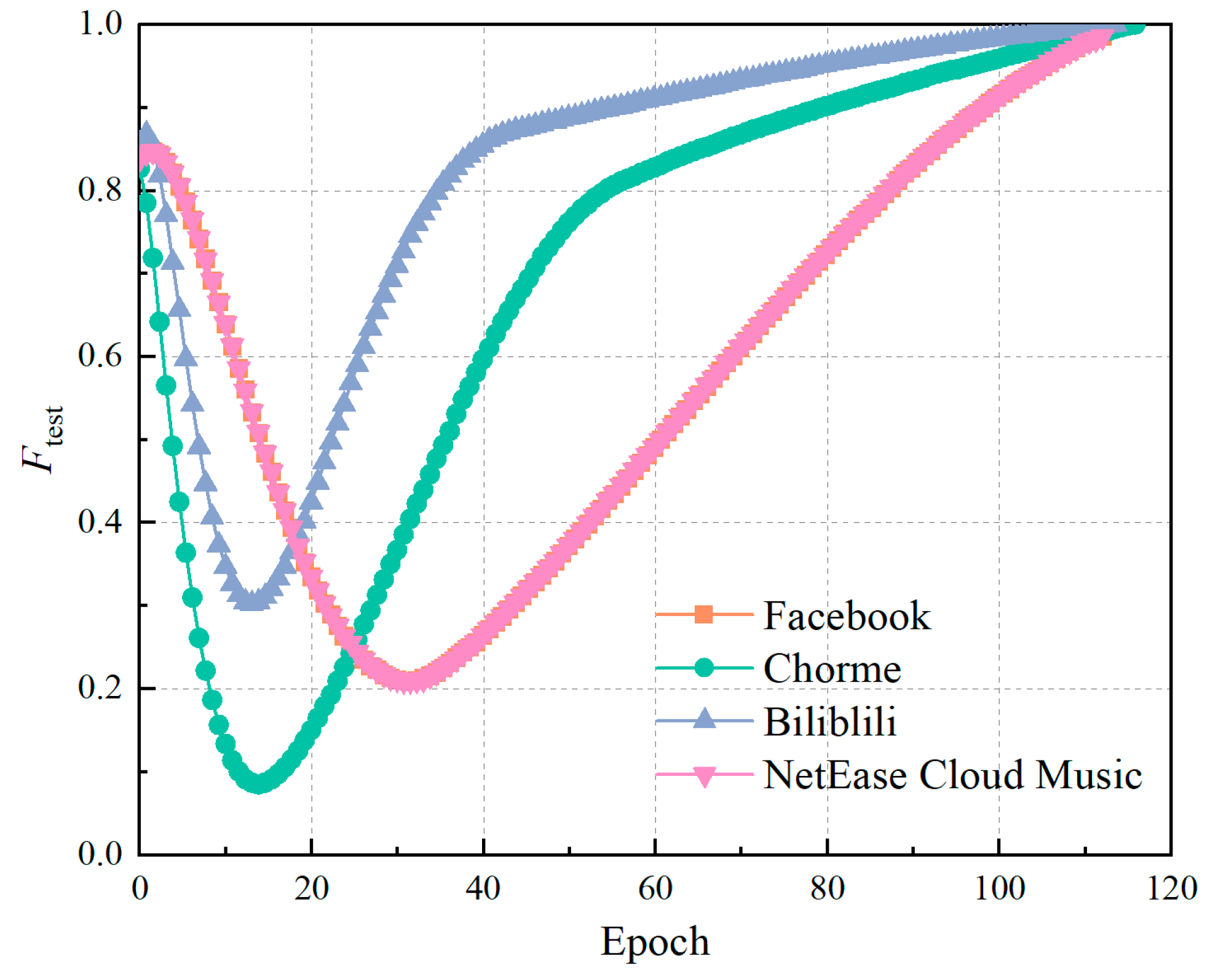
The support vector machine (SVM) classification algorithm is capable of making classification decisions based on traffic feature values. To improve the generalization ability of the SVM algorithm, the 20,000 datasets were first dimensionally reduced. The SVM classifier was trained and learned using the k-fold (k=10) cross-validation method. The convergence diagram for the training process of the SVM's prediction accuracy for each category is presented in Figure 8.
As shown in Figure 8, the support vector machine (SVM) exhibits a robust performance during training and effectively handles high-dimensional datasets. The training process terminates upon reaching 117 iterations. Moreover, the SVM demonstrates the capacity to generalize well and process novel data efficiently. Figure 9 illustrates the distribution of prediction accuracy tests for each category conducted using the SVM.
The Support Vector Machine (SVM) achieved an overall accuracy of 80.95% across the four applications of Facebook, Chrome, Bilibili, and NetEase Cloud Music, with accuracy rates of 77.57%, 87.69%, 78.40%, and 80.88%, respectively. Figure 9 reveals that the SVM algorithm produces a relatively low error rate for overall classification, albeit with uneven accuracy across different application types. However, SVMs exhibit sensitivity to parameter and kernel function selection, resulting in higher classification bias.

4.3. Results of neural network

The neural network starts by initializing the weights of all neuron nodes, which generates an output through forward propagation. Subsequently, the deviation is computed by combining actual and predicted output values, allowing all neurons to update their weights via reverse backpropagation. Following multiple rounds of experimental debugging, we set the learning rate at 0.0001 and the number of iterations at 20 for training the neural network algorithm using 20,000 samples, as demonstrated in Figure 10.
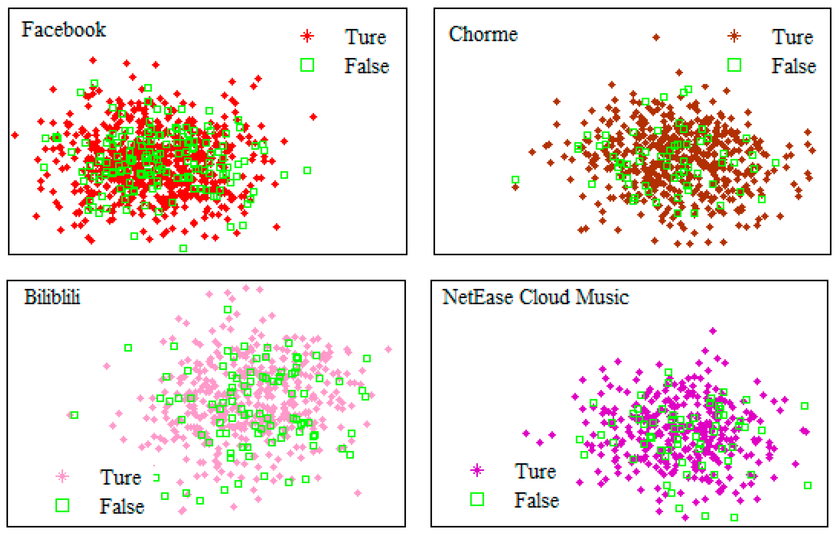
Figure 10 demonstrates that the neural network can effectively address complex non-linear problems and exhibits robust fault tolerance. Training achieved the target in 128 steps, allowing for a certain degree of noise and error during the process while producing minimal error fluctuations in test samples. Moreover, the neural network can dynamically adjust its weights and biases, making it adaptable to diverse datasets. Figure 11 displays the results of testing the trained neural network model on test samples.
The neural network algorithm achieved an accuracy of 92.29%, 93.27%, 90.00%, and 96.26% for Facebook, Chrome, Bilibili, and NetEase Cloud Music applications, respectively, resulting in an overall accuracy of 91.75%. Appropriate parameters such as network structure, learning rate, and activation function were selected for the neural network's learning process. The training produced highly accurate results that were consistent across different software, with only low differences in accuracy rates.

4.4. Effect of training samples on test accuracy

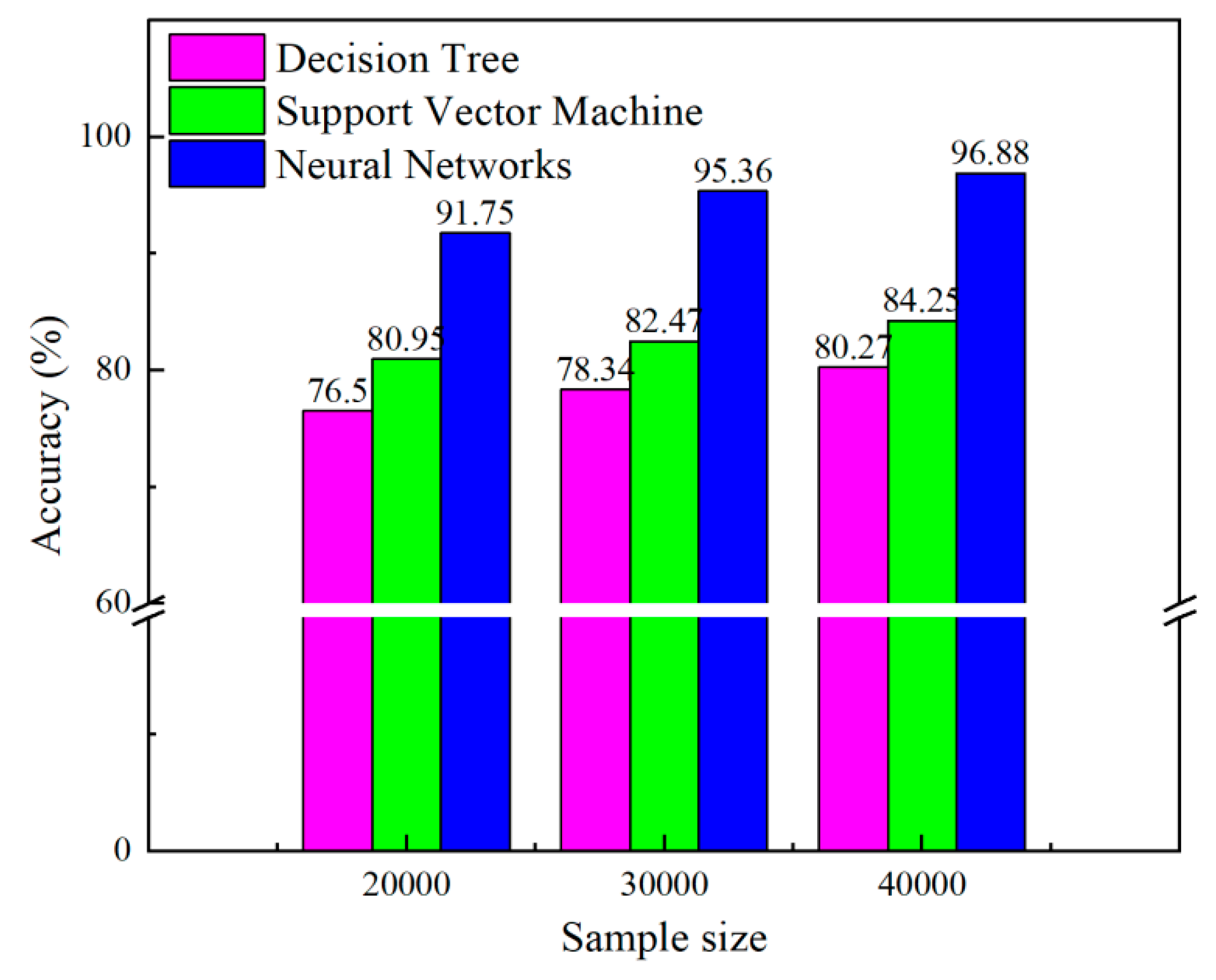
Based on the model architectures of the three algorithms, we further trained 30,000 and 40,000 samples using the same training parameters and feature selection process. Then, we classified 2,000 test samples using the trained models and compared the results with the model trained with 30,000 and 40,000 samples. Figure 12 summarizes the accuracy of the three algorithms in classifying test samples with different training sample sizes.
As shown in Figure 12, the decision tree algorithm's accuracy increases from 76.5% to 80.27% as the number of training samples increases from 20,000 to 40,000. Similarly, the support vector machine algorithm's accuracy increases from 80.95% to 84.25%, and the neural network algorithm's accuracy increases from 91.75% to 96.88%. This indicates that increasing the number of training samples significantly improves the accuracy of all three algorithms. Among the three algorithms, the neural network algorithm stands out as it can use the multi-layer neuron structure to learn complex non-linear relationships and handle non-linear problems more effectively than the other two algorithms.

5. Conclusions

A machine learning-based method for classifying digital media traffic is proposed in this paper. The method learns and classifies features of digital media application data to predict traffic of four applications: Facebook, Chrome, Bilibili, and NetEase Cloud Music. Experimental results show that the proposed method is effective in classification and prediction, and can be applied in various scenarios, such as web traffic management, advertising recommendation, and content distribution. The main conclusions of the study are summarized below:
(1) The decision tree algorithm exhibits significant errors in overall classification and inconsistent accuracy across application types. Additionally, it is highly prone to overfitting during the classification process and is susceptible to errors due to noisy data.
(2) Although the support vector machine algorithm exhibits lower error rates in overall classification, its accuracy across application types varies considerably. This is due to its sensitivity to the choice of parameters and kernel functions, which can introduce significant bias into the classification process.
(3) The neural network algorithm had higher accuracy for the classification of four applications, Facebook, Chorme, Bilibili and NetEase Cliud Music, and was consistent with less variation in accuracy across software.
(4) The classification accuracy of all three algorithms significantly improves with increasing training samples. Notably, the neural network algorithm shows the largest increase in accuracy, reaching 96.88% with a substantial training sample size of 40,000 data streams, thereby demonstrating the efficacy of the proposed optimization method. The neural network algorithm is particularly adept at managing high-dimensional data and can effectively handle datasets with a large number of features.

6. Patents

This section is not mandatory but may be added if there are patents resulting from the work reported in this manuscript.

Funding

This research was funded by “Research on Traditional Culture Based on Digital Media”(No:20200402047).

References

  1. Dainotti, A.; Pescapé, A.; Claffy, K.C. Issues and Future Directions in Traffic Classification. IEEE Netw. 2012, 26, 35–40. [Google Scholar] [CrossRef]
  2. Park, B.; Won, Y.J.; Chung, J.Y.; Kim, M.S.; Hong, J.W.K. Fine-Grained Traffic Classification Based on Functional Separation. Int. J. Netw. Manag. 2013, 23, 350–381. [Google Scholar] [CrossRef]
  3. Salman, O.; Elhajj, I.H.; Kayssi, A.; Chehab, A. A Review on Machine Learning-Based Approaches for Internet Traffic Classification. [CrossRef]
  4. Lotfollahi, M.; Jafari Siavoshani, M.; Shirali Hossein Zade, R.; Saberian, M. Deep Packet: A Novel Approach for Encrypted Traffic Classification Using Deep Learning. Soft Comput. 2020, 24, 1999–2012. [Google Scholar] [CrossRef]
  5. Zhu, D.; Jin, H.; Yang, Y.; Wu, D.; Chen, W. DeepFlow: Deep Learning-Based Malware Detection by Mining Android Application for Abnormal Usage of Sensitive Data. Proc. - IEEE Symp. Comput. Commun. 2017, 438–443. [Google Scholar] [CrossRef]
  6. Erman, J.; Mahanti, A.; Arlitt, M.; Williamson, C. Identifying and Discriminating between Web and Peer-to-Peer Traffic in the Network Core. 16th Int. World Wide Web Conf. WWW2007 2007, 883–892. [Google Scholar] [CrossRef]
  7. Williams, N.; Zander, S.; Armitage, G. A Preliminary Performance Comparison of Five Machine Learning Algorithms for Practical IP Traffic Flow Classification. ACM SIGCOMM Comput. Commun. Rev. 2006, 36, 7–15. [Google Scholar] [CrossRef]
  8. Zhang, C.; Wang, X.; Li, F.; He, Q.; Huang, M. Deep Learning–Based Network Application Classification for SDN. Trans. Emerg. Telecommun. Technol. 2018, 29, e3302. [Google Scholar] [CrossRef]
  9. Ng, B.; Hayes, M.; Seah, W.K.G. Developing a Traffic Classification Platform for Enterprise Networks with SDN: Experiences and Lessons Learned.
  10. Wang, W.; Sheng, Y.; Wang, J.; Zeng, X.; Ye, X.; Huang, Y.; Zhu, M. HAST-IDS: Learning Hierarchical Spatial-Temporal Features Using Deep Neural Networks to Improve Intrusion Detection. [CrossRef]
  11. Wu, K.; Chen, Z.; Li, W. A Novel Intrusion Detection Model for a Massive Network Using Convolutional Neural Networks. IEEE Access 2018, 6, 50850–50859. [Google Scholar] [CrossRef]
  12. Rezaei, S.; Liu, X. Deep Learning for Encrypted Traffic Classification: An Overview. IEEE Commun. Mag. 2019, 57, 76–81. [Google Scholar] [CrossRef]
  13. Murthy, S.K. Automatic Construction of Decision Trees from Data: A Multi-Disciplinary Survey. Data Min. Knowl. Discov. 1998 24 1998, 2, 345–389. [Google Scholar] [CrossRef]
  14. Safavian, S.R.; Landgrebe, D. A Survey of Decision Tree Classifier Methodology. IEEE Trans. Syst. Man Cybern. 1991, 21, 660–674. [Google Scholar] [CrossRef]
  15. Lu, H.; Ma, X. Hybrid Decision Tree-Based Machine Learning Models for Short-Term Water Quality Prediction. Chemosphere 2020, 249, 126169. [Google Scholar] [CrossRef] [PubMed]
  16. Rizvi, S.; Rienties, B.; Khoja, S.A. The Role of Demographics in Online Learning; A Decision Tree Based Approach. Comput. Educ. 2019, 137, 32–47. [Google Scholar] [CrossRef]
  17. Sheykhmousa, M.; Mahdianpari, M.; Ghanbari, H.; Mohammadimanesh, F.; Ghamisi, P.; Homayouni, S. Support Vector Machine Versus Random Forest for Remote Sensing Image Classification: A Meta-Analysis and Systematic Review. IEEE J. Sel. Top. Appl. Earth Obs. Remote Sens. 2020, 13, 6308–6325. [Google Scholar] [CrossRef]
  18. Cervantes, J.; Garcia-Lamont, F.; Rodríguez-Mazahua, L.; Lopez, A. A Comprehensive Survey on Support Vector Machine Classification: Applications, Challenges and Trends. Neurocomputing 2020, 408, 189–215. [Google Scholar] [CrossRef]
  19. Raj, J.S.; Ananthi, J.V. RECURRENT NEURAL NETWORKS AND NONLINEAR PREDICTION IN SUPPORT VECTOR MACHINES. J. Soft Comput. Paradig. (JSCP 2019. [Google Scholar] [CrossRef]
  20. Pan, Y.; Zhou, P.; Yan, Y.; Agrawal, A.; Wang, Y.; Guo, D.; Goel, S. New Insights into the Methods for Predicting Ground Surface Roughness in the Age of Digitalisation. Precis. Eng. 2021, 67, 393–418. [Google Scholar] [CrossRef]
  21. Pan, Y.; Wang, Y.; Zhou, P.; Yan, Y.; Guo, D. Activation Functions Selection for BP Neural Network Model of Ground Surface Roughness. J. Intell. Manuf. 2020, 31, 1825–1836. [Google Scholar] [CrossRef]
  22. Yu, X.; Prevedouros, P.D. Performance and Challenges in Utilizing Non-Intrusive Sensors for Traffic Data Collection. Adv. Remote Sens. 2013, 2013, 45–50. [Google Scholar] [CrossRef]
  23. Lan, H.; Zhu, X.; Sun, J.; Li, S. Traffic Data Classification to Detect Man-in-the-Middle Attacks in Industrial Control System. Proc. - 2019 6th Int. Conf. Dependable Syst. Their Appl. DSA 2019 2020, 430–434. [Google Scholar] [CrossRef]
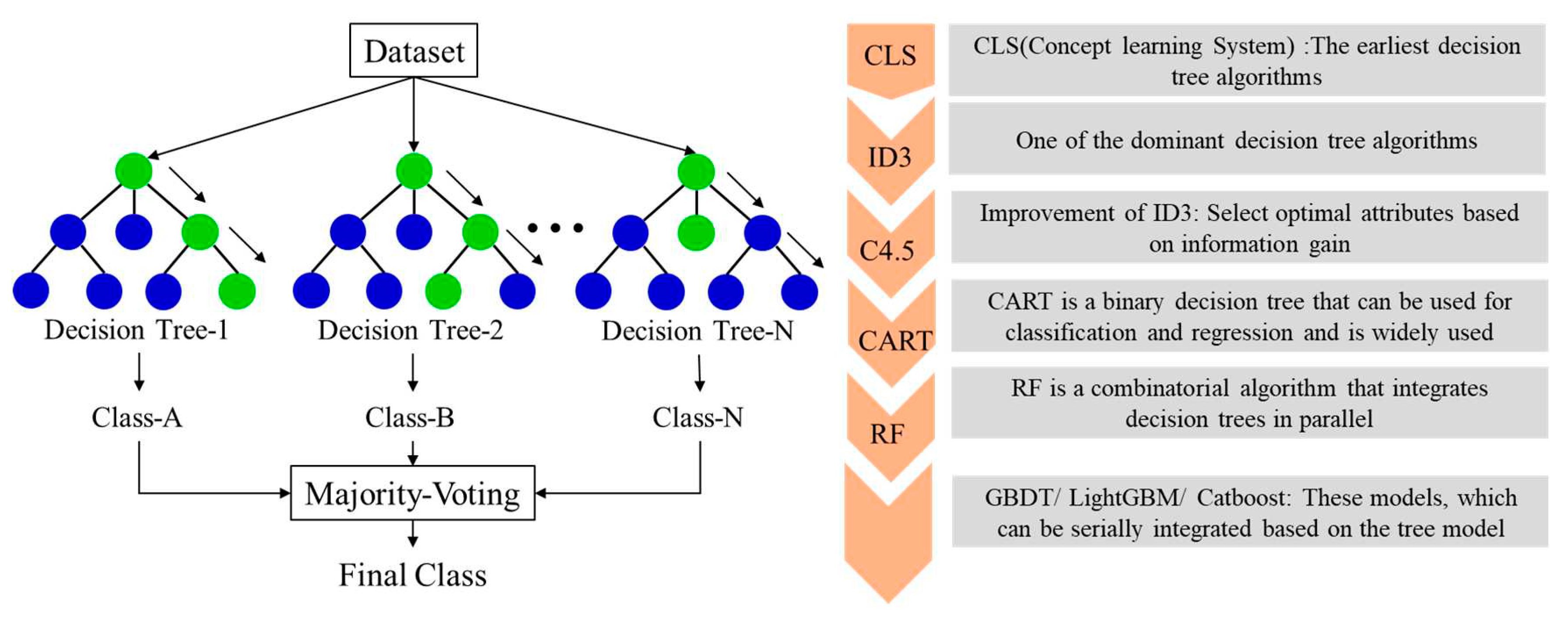
Figure 1. Schematic diagram and mainstream algorithms for decision trees.
Preprints 71256 g001
Figure 2. Schematic diagram and mainstream algorithms for support vector machine (SVM).
Preprints 71256 g002
Figure 3. Schematic diagram and mainstream algorithms for BP neural network (BPNN).
Preprints 71256 g003
Figure 4. Schematic diagram of the proposed method.
Preprints 71256 g004
Figure 5. Schematic diagram of the Data pre-processing.
Preprints 71256 g005
Figure 6. The training process of the decision tree algorithm.
Preprints 71256 g006
Figure 7. Classification of test samples by the decision tree algorithm.
Preprints 71256 g007
Figure 8. The training process of the SVM.
Preprints 71256 g008
Figure 9. Classification of test samples by the support vector machine algorithm.
Preprints 71256 g009
Figure 10. Training process of the neural network algorithm.
Preprints 71256 g010
Figure 11. Classification of test samples by neural network algorithm.
Preprints 71256 g011
Figure 12. Accuracy of the three algorithms in classifying test samples with different training sample sizes.
Preprints 71256 g012
Table 1. Application type datasets for training and test samples.
Application type Training samples 1 Training samples 2 Training samples 3 Training samples 4 Proportion
Facebook 7000 10500 14000 700 35%
Chorme 5200 7800 10400 520 26%
Biliblili 4400 6600 8800 440 22%
NetEase Cloud Music 3400 5100 6800 340 17%
Total 20000 30000 40000 2000 100%
Disclaimer/Publisher’s Note: The statements, opinions and data contained in all publications are solely those of the individual author(s) and contributor(s) and not of MDPI and/or the editor(s). MDPI and/or the editor(s) disclaim responsibility for any injury to people or property resulting from any ideas, methods, instructions or products referred to in the content.
Copyright: This open access article is published under a Creative Commons CC BY 4.0 license, which permit the free download, distribution, and reuse, provided that the author and preprint are cited in any reuse.
Prerpints.org logo

Preprints.org is a free preprint server supported by MDPI in Basel, Switzerland.

Subscribe

© 2024 MDPI (Basel, Switzerland) unless otherwise stated