1. Introduction
Synthetic Aperture Radar (SAR) is a kind of active earth-observation system which can produce high-resolution image all day, has been widely used in ground observation and military reconnaissance. One of its primary applications is the detection and identification of various military targets [
1,
2]. With the enhancement of SAR data acquisition capability, Synthetic Aperture Radar Automatic Target Recognition (SAR ATR) [
3] has become a key technology and research hotspot of radar signal processing. Traditional SAR target recognition methods [
4] merely rely on artificial experience for feature extraction and selection, which lead to a certain degree of subjectivity and bias. Additionally, it is challenging to guarantee the effectiveness of recognition results [
5]. In recent years, deep learning methods [
6], especially Convolutional Neural Networks (CNN), have been extensively used in computer vision [
7,
8] and demonstrating remarkable achievements. Meanwhile, based on deep learning, the image processing method has also been successfully extended to the field of remote sensing images [
9,
10], presenting a new direction and breakthrough for SAR target recognition [
11,
12,
13].
At present, CNN has become one of the most effective network architecture for image recognition tasks. As the earliest CNN network, LeNet-5, proposed by LeCun et al. [
14] in 1998 for handwritten digit recognition, was regarded as the first CNN structure. Over time, researchers have continuously refined and optimized the classic CNN architecture and its features, leading to the design of more complex and high-performing CNNs, such as Alexnet [
15], GoogLeNet [
16], VGGNet [
17], Resnet [
18], etc. Despite the outstanding performance achieved by classic CNN structures, the neural network has a low level of transparency and is also known as the black boxes [
19] due to the lack of a clear visual explanation for the representation of internal features and parameter organization. These limitations significantly constrain people’s ability to understand and interpret the internal workings of neural networks, consequently restricting their potential applications in specialized fields, such as medicine, finance, transportation, military, and other domains [
20,
21]. There are currently two primary research directions for interpretability, which are Intrinsic Explanation and Post-hoc Explanation [
22]. Intrinsic Explanation aims to enhance the interpretability of the model itself, enabling users to understand the calculating process and rationale without requiring additional information or algorithms. In contrast, Post-hoc Explanation mainly focuses on explaining the behavior and decision-making process of black-box models [
23]. Retraining the model can be too costly in terms of time and resources since the model has already been trained and deployed. As such, the Post-hoc Explanation approach is often more appropriate in such cases. Representation visualization, as an intuitive method in post-hoc interpretation, mainly involves combining the input, middle layer parameters, and output information of the pre-trained model to achieve an interpretation of the decision results. Gradient-based methods, Perturbation, and Class Activation Map (CAM) are three widely adopted methods for achieving representation visualization [
22,
24].
The gradient-based method [
25,
26,
27,
28,
29,
30,
31] backpropagates the gradients of a specific class into the input image to highlight image regions that contribute positively or negatively to the result. The methods are fast computation and high resolution of the generated images but usually suffer from excessive noise. CAM is one class of the most important methods specifically designed for CNNs [
24,
32,
33,
34,
35,
36,
37]. The method utilizes the form of a heatmap to visually highlight the regions most relevant to the particular category. The CAM-based method was first proposed by Zhou et al. [
33] in 2016. They believed that with the deepening of CNN layers, the feature map of the intermediate layer contains less and less irrelevant information, and the last convolutional layer of the CNN achieves the highest-level semantic information. After that, numerous CAM methods have been proposed, including Grad-CAM [
34], Grad-CAM++ [
35], Grad-CAM [
36], Group-CAM [
32], Score-CAM [
24], Ablation-CAM [
37], etc. Although these methods have demonstrated good performance in image interpretation, they may suffer from low resolution and spatial precision in some cases. Interpretability methods based on perturbation [
38,
39,
40,
41] typically utilize the element-wise product of generated masks and the original image to obtain the perturbed input images, which are then fed into the model to observe the changes in the prediction result. The information generated is used to optimize the weighted mask to obtain the final interpretation result image. Among them, RISE [
41] randomly generates a large number of masks through Monte Carlo sampling method to occlude different parts of the input image. And the final saliency map is generated by the weighted sum of the masks and the scores predicted by the base model on the masked images.
In this paper, we propose a post-hoc interpretation method of black-box models for SAR ATR called Randomized Input Sampling for explanation based on Clustering (C-RISE). We demonstrate the effectiveness of C-RISE through extensive experimental validation and comparative analysis. Specifically, our method exhibits superior performance when dealing with SAR images that suffer from severe noise interference, as well as cases where adjacent pixels exhibit mutual influence and dependence. C-RISE offers several advantages over other neural network interpretable algorithms, including white-box methods:
- 1.
The method is a black-box interpretation method, and the calculation process does not need to use the weight, gradient, feature map and other information of the model so that it has better robustness and transferability. Furthermore, the approach avoids errors caused by unreasonable weight selection and information loss during feature map upsampling in Class Activation Mapping (CAM) methods;
- 2.
Compared with RISE, our algorithm can group mask images that capture similar fusion features into different groups by clustering strategy. This allows for the concentration of more energy in the heatmap on the target area, thereby increasing the interpretability of the model.
- 3.
C-RISE employs Gaussian blur to process masked regions, as opposed to simply setting occluded pixels to 0. This technique ensures the consistency and integrity of the original image structure while covering certain areas. As a result, it reduces the deviation of network confidence caused by the destruction of spatial structure, leading to more credible results when compared to other perturbation-based interpretation methods.
The contents of this article are organized as follows: In
Section 2, we introduce the principle of the RISE algorithm and CAM methods.
Section 3 elaborates on the details of the C-RISE algorithm.
Section 4, we verify the effectiveness and robustness of the proposed method through both qualitative judgment and quantitative description. Finally, in
Section 5, we discuss the experimental results, clarify any confusion, and explore potential future work.
2. Related Work
In this section, we first review the existing classical methods of CAM [
24,
32,
33,
34,
35,
36,
37] and the RISE [
41] algorithm. Since both CAM methods and RISE interpretation methods display in the form of heatmaps, we focus our subsequent experiments [
41] on comparing the effects of different CAM methods, RISE, and C-RISE. This chapter provides theoretical support for the design and experimentation of C-RISE.
2.1. CAM Methods
Zhou et al. [
33] proposed the Class Activation Map (CAM) method which utilizes the final convolutional layer of CNN to extract the most abstract target-level semantic information. Its corresponding feature map contained the most abstract target-level semantic information and each channel detected different activated parts of the target. Thus, the class activation map relevant to the recognition result of class
c can be generated by the channel-wise weighted summation of the final feature maps. The formal representation of this process can be expressed as follows:
where
represents the connection weight of the
kth neuron pair classified as class
c in the Softmax layer, and
represents the feature map of the
kth channel in the
lth convolutional layer. The disadvantage of this method is that it can only be applied to the last layer feature map and the full connection is GAP operation. Otherwise, it requires the user to modify the network and retrain, and such costs are sometimes substantial. To overcome the disadvantages, Selvaraju et al. [
34] proposed a method named Grad-CAM and updated the weight generation method in Equation (
1) as follows:
where the sum element is the gradient of the calculated class score(
) with respect to the pixel values at each position of
, and
Z represents the normalization factor. Compared to the CAM method, Grad-CAM is more generalized and can be used for different model structures. Both Grad-CAM++[
35] and XGrad-CAM [
36] are improved algorithms based on Grad-CAM method. The basic form of Grad-CAM++ is the same as Grad-CAM, but the difference is that the combination of higher-order gradients is used as the channel weight in Grad-CAM, which improves the visualization effect of multi-object images and the positioning is more accurate. XGrad-CAM achieves better visualization of CNN decisions through a clear mathematical interpretation.
Different from the improvement idea based on gradient, Score-CAM [
24] is a gradient-free algorithm for visualizing CNN decisions. It defines the concept of Increase of Confidence (CIC), which measures the increment of confidence relative to a baseline image. The CIC score for a particular feature map
is computed as:
where
is the input image, ∘ represents the Hadamard product, and
is the baseline image, which can be set to an all-0 matrix with the same size as the original image.
denotes the neural network’s output score for the target class. The algorithm then computes CIC scores for all feature maps in a particular layer and updates the scores using the Softmax operation. These updated scores are used as the weights for the corresponding feature maps. Finally, the different feature maps are weighted and summed to generate a visual image.
The CAM approach has been demonstrated to be effective in visualizing the important regions of objects in various optical image datasets. However, when applied to Synthetic Aperture Radar (SAR) images, several challenges arise such as gradient dispersion, energy unconcentration, and inaccurate positioning. These challenges are primarily due to the unique characteristics of SAR images which include:
- 1.
SAR images are often characterized by low resolution and low Signal-to-Noise Ratio (SNR), which makes it challenging to visualize important features and information accurately. Additionally, the imaging principle of SAR images is based on active imaging, which introduces a significant amount of interference spots in the image, thereby making SAR images significantly different from optical images. These interference spots can significantly impact the visualization process, leading to inaccurate feature localization and reduced effectiveness of CAM-based visualization methods;
- 2.
The relatively small difference between different categories in SAR image datasets poses a challenge to visualization techniques such as CAM, which heavily rely on distinguishing features between different categories. Furthermore, the target area of SAR images is often highly localized, which makes accurate positioning critical for the interpretation of visualizations. However, different CAM methods typically use feature maps to upsample to the size of the original image, which can introduce positioning deviations. Despite ongoing efforts to generate high-resolution feature maps, the visualization effect of SAR images using CAM methods remains suboptimal.
2.2. RISE
Randomized Input Sampling for Explanation (RISE) [
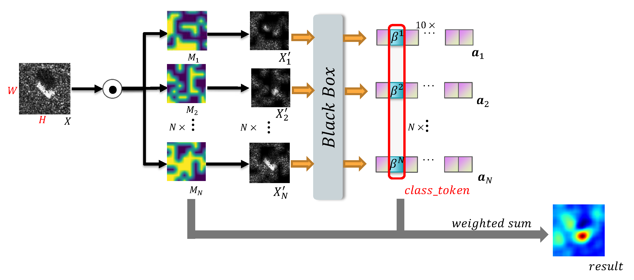
41] is a perturbation-based visualization method in local interpretation, which is, for the prediction result of a single image, a heatmap with prominent areas is obtained as the interpretation result by combining randomly sampled masks. The detailed architecture of RISE is presented in
Figure 1. Firstly, based on Monte Carlo sampling method, a large number of masks with the same size as the original image are generated. After that, the element-wise product of masks and the original image are made to obtain the corresponding perturbed images. Then, the masked images were input into the black-box model to obtain the prediction probability of the inferred category. Finally, the prediction probability is used as the weight to sum the masks, so as to superimpose the areas in the original image that play an important role in the specified category. Randomized Input Sampling for Explanation (RISE) [
41] is a perturbation-based method that generates a heatmap to highlight the important regions of an input image with respect to the prediction of a black-box model. The detailed architecture of RISE is presented in
Figure 1. RISE generates a large number of randomized binary masks and applies them to the input image to obtain a set of masked images. The CNN is then applied to each masked image to obtain a set of output scores. The final explanation map is generated by aggregating the scores obtained from all the masked images. RISE has been shown to be effective in providing local interpretability for various image classification models. Moreover, Score-CAM is a gradient-free method that is inspired by RISE [
24].
RISE method is a black-box interpretation method, which does not need to use the weight, gradient, feature map and other information in the calculation process. Since the Monte Carlo sampling method is a stochastic approximate inference method, the idea of this method is to find the expected value of the function
under the complex probability distribution
, as shown in Equation (
4).
In the RISE algorithm, the predicted probability of the black-box model for the category to which the perturbed image belongs can be viewed as the importance of the region retained by the mask. Then the importance of the prominent region of the final generated image can be viewed as the expectation obtained from all masks, as shown in Equation (
5).
where
denotes the pixel with a value of 1 in the mask, and
represents the expected score obtained by inputting the pictures under different masks
M into the model
.
can be intuitively interpreted as the greater the prediction probability after the pixel-wise multiplication of the mask and the image, the more important the region retained by this mask.
Then, we can expand the expression according to the definition of expectation as follows:
where
By substituting Equation (
7) into Equation (
6), we can get:
Since the mask
m has a 0-1 distribution, we can obtain Equation (
9):
It can be seen from Equation (
11) that the heatmap can be obtained by the sum of masks obtained from random sampling by weighting, while the weight is the predicted probability of the perturbed image. When masks are sampled by uniform sampling,
can be expressed as:
So Equation (
10) can be updated to:
Considering that pixle-wise masks can cause huge changes in the prediction of the model, and the computational cost of sampling a pixle-level mask is exponential, during mask generation, small masks are generated first and then upsampled back to the image size in order to ensure smoothness.
3. Our Method
As a post-hoc interpretation algorithm based on perturbation, RISE algorithm has a more intuitive and understandable presentation than the visual interpretation method based on back propagation. At the same time, RISE also overcomes the limitations of general CAM methods by avoiding the generation of unreasonable weights and the problem of small feature maps during the up-sampling process. However, the effectiveness of RISE and other optical image-based interpretive methods in SAR ATR scenarios is limited. This is because the active imaging mechanism of SAR images results in multiplicative noise, which causes problems such as noise, energy dispersion, and inaccurate positioning when applying optical image-based interpretive methods to SAR image recognition [
3,
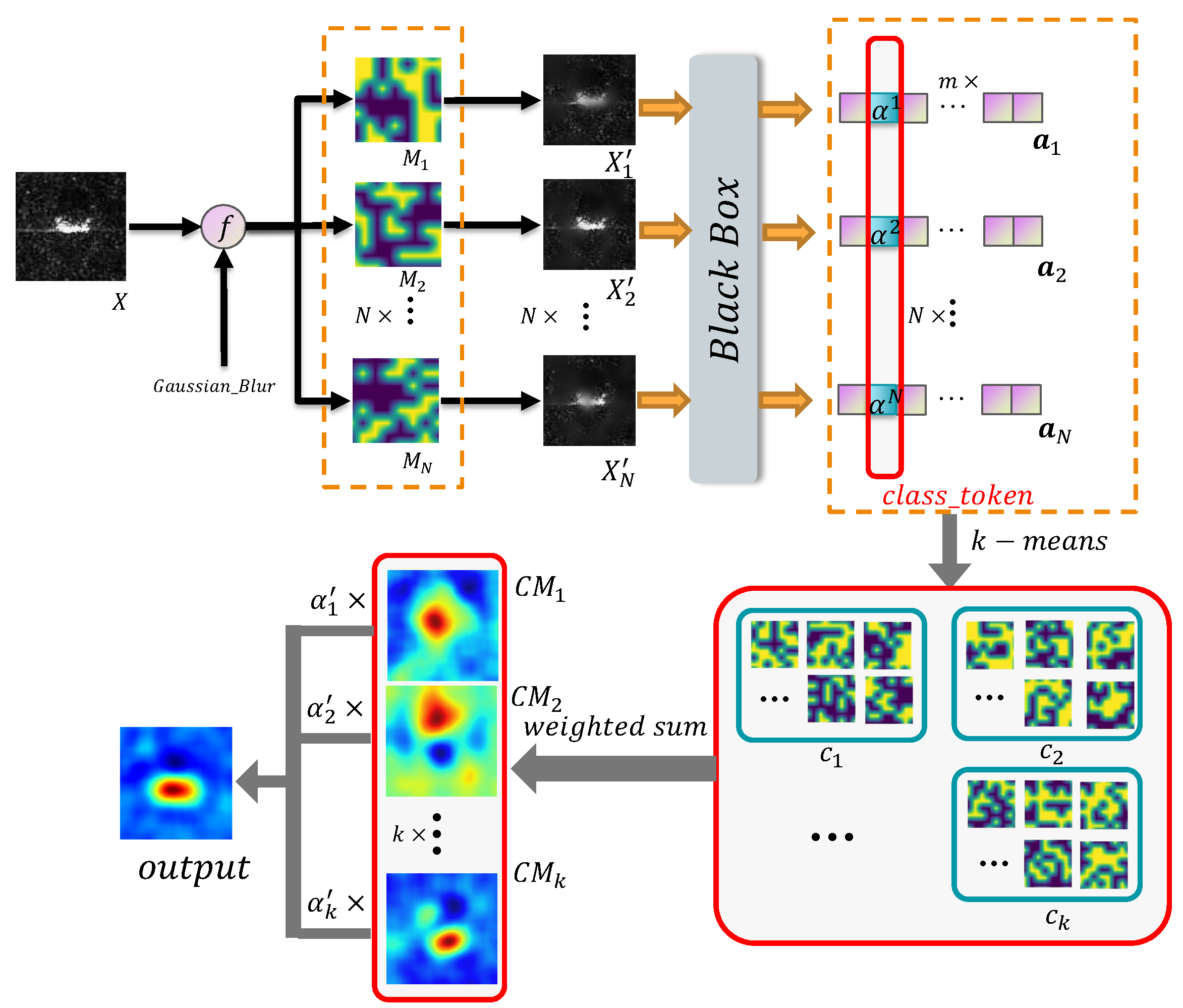
4]. To address this issue, we propose an algorithm based on RISE, called Randomized Input Sampling for Explanation based on Clustering (C-RISE), which is a post-hoc interpretation method for black-box models in SAR ATR. Our algorithm considers the structural consistency and integrity of SAR images and highlights the regions that contribute to category discrimination in SAR images.
Figure 2 illustrates the workflow of our proposed approach.
3.1. Mask Generation
As shown in
Section 2.2, pixle-level occlusion may have a huge impact on the model, and the computational complexity of sampling is high. Therefore, in order to ensure the smoothness and the consistency of the target space structure when generating masks, small masks are generated first and then upsampled back to the image size. The basic process is shown in
Figure 3. Formally, the process of generating masks can be described as follows:
- 1.
N binary masks , , are randomly generated based on Monte Carlo sampling, where . s is smaller than image size H and W. In , each element independently to 1 with probability p and to 0 with the remaining probability;
- 2.
Upsample to ;
- 3.
A rectangular area was randomly selected from as , where .
After obtaining
N masks, we introduce Gaussian blur to the occluded part of the original image, which is in order to make the image after the mask processing can retain the maximum consistency of the original image, and smoothly occlusion of the region. Gaussian blur is an image blurring filter that computes the transformation of each pixel in an image with a normal distribution. The normal distribution equation in 2-dimensional space can be written as:
where
denotes the pixel position and
means the standard deviation of the normal distribution. It is worth noting that in 2-dimensional space, the contours of the surface generated by Equation (
13) are normally distributed concentric circles from the center. The value of each pixel is a weighted average of the neighboring pixel values. The value of the original pixel has the largest Gaussian distribution value, so it has the largest weight, and the neighboring pixels get smaller and smaller as they get farther from the original pixel. The Gaussian blur preserves the edge effect more than other equalization blur filters, which is equivalent to a low-pass filter.
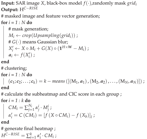
Based on Gaussian blur, We can use Equation (
14) to obtain the image after mask processing:
where
denotes the original image,
means an all-1 matrix and its shape is
.
3.2. Clustering
The masked image
,
,
are input to the black-box model
to obtain the output vector
,
,
. Moreover, we use
as the feature vectors to cluster
by
k-
.
m is the number of categories. The process is shown in Equations (
15)–(
17).
where
denotes the
ith cluster,
denotes the
jth mask in
ith cluster,
k and
represent the number of clusters and the number of elements in the
ith cluster, respectively.
If the original image is identified as class
l after the black-box model, we can obtain:
where
denotes the feature vector from
and
can be seen as the contribution of the
jth mask in the
ith cluster to the model. After that, we use
to estimate the weight of a specific mask and calculate the weighted sum in each cluster
as follows:
After that, we calculated the
value of
through Equation (
3) and used it as the classificatory information that
was concerned about. Finally, the final result
is generated by weighted summation of the feature maps of different clusters. The process is formulated as Equations (
20) and (
21). The pseudo-code is presented in Algorithm 1.
|
Algorithm 1: C-RISE |
 |
4. Experiment
4.1. Experimental Settings
This study employs SAR images of ten vehicle target types under standard operating conditions (SOC) from the Moving and Stationary Target Acquisition and Recognition (MSTAR) dataset [
42] as the experimental data. The dataset comprises 5172 SAR images with dimensions of
, with 2536 images used for training and 2636 for testing. The ten target categories include
,
,
,
,
,
,
,
,
, and
.
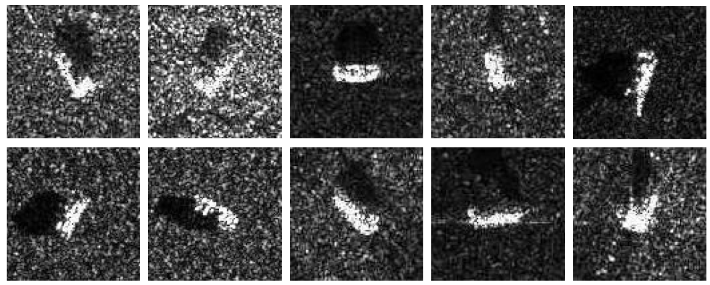
Figure 4 displays ten representative SAR images for each category.
During the experiment, the Alexnet model [
5] was utilized as a classifier, and its structure is depicted in
Figure 5. It is worth mentioning that, as the C-RISE algorithm is primarily tailored for black-box models, alternative efficient models may be employed in place of Alexnet. After conducting multiple iterations of training, the neural network achieved a recognition rate of 97.6%, which indicates the effectiveness of using various methods to generate saliency maps. However, since this paper primarily focuses on interpreting and analyzing the network structure using different visualization methods, the training techniques and processes are not extensively discussed. During the implementation of the C-RISE algorithm, several parameters were set, including
,
,
,
. It should be emphasized that the experimental results were sensitive to the number of clusters, and selecting
or 8 yielded relatively optimal results. Hence, for the purpose of this paper,
k was specified as 4.
4.2. Class Discriminative Visualization
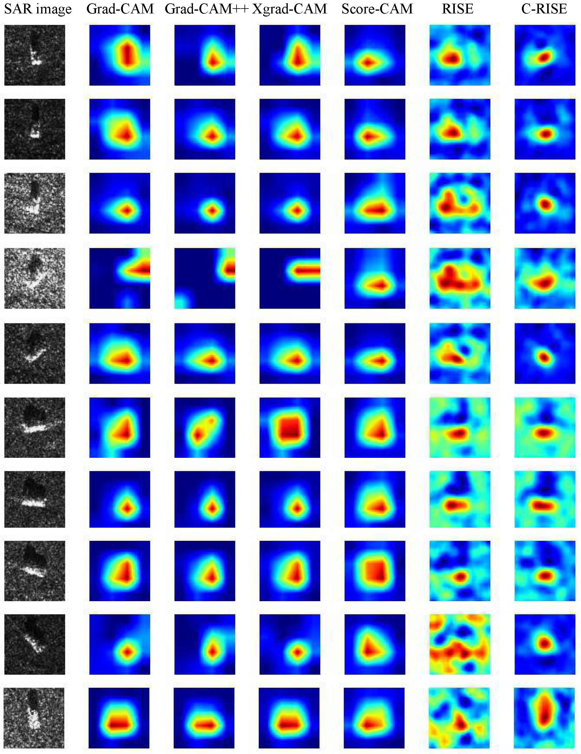
Since the class activation map generated by CAM method and the saliency map generated by C-RISE algorithm are presented in the form of heatmap, we focus on comparing the experimental effects of different CAM methods, RISE algorithm and C-RISE algorithm in the following experimental part, referring to the comparison method in [
41]. In this section, we randomly selected ten graphs that were correctly classified in different networks from the testset, and used Grad-CAM [
34], Grad-CAM++ [
35], XGrad-CAM [
36], Score-CAM [
24], RISE [
41] and C-RISE to visually analyze the model recognition process, and the comparison is shown in
Figure 6.
We can verify the fairness and localization ability of the C-RISE algorithm from a qualitative and quantitative perspective. It can be intuitively seen from
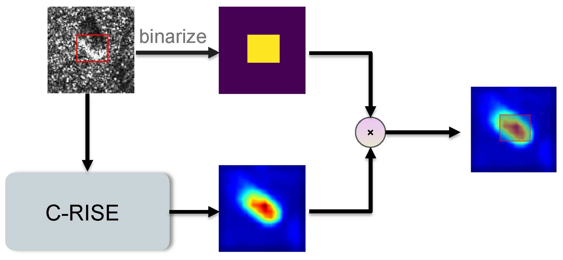
Figure 1 that compared with CAM methods and RISE, the highlighted areas of the heatmap generated by our method are more closely concentrated near the target and the degree of energy dispersion is smaller. The heatmap is an image composed of different color intensities, and the intensity of a pixel’s color corresponds to its importance. Analyzing from a quantitative point of view, we measure the quality of the saliency map by the localization ability. From an energy-based perspective, we are concerned with how much energy of the salient map falls in the bounding box of the target object. Therefore, we adopted a similar measure to [
24], the specific process is shown in
Figure 7. Firstly, we annotated the bounding boxes of the objects of all images in testset, and then binarized the images according to the rule that the inner region of the bounding box is set to 1, and the outer region is 0. The processed image is then multiplied by the heatmap and summed to obtain the energy within the target bounding box. We use the ratio of the internal energy of the bounding box to the total energy of the heatmap
to measure the localization and recognition capabilities of different methods. The mathematical expression is shown in Equation (
22).
where
denotes the energy value of the pixel at position
in the heatmap.
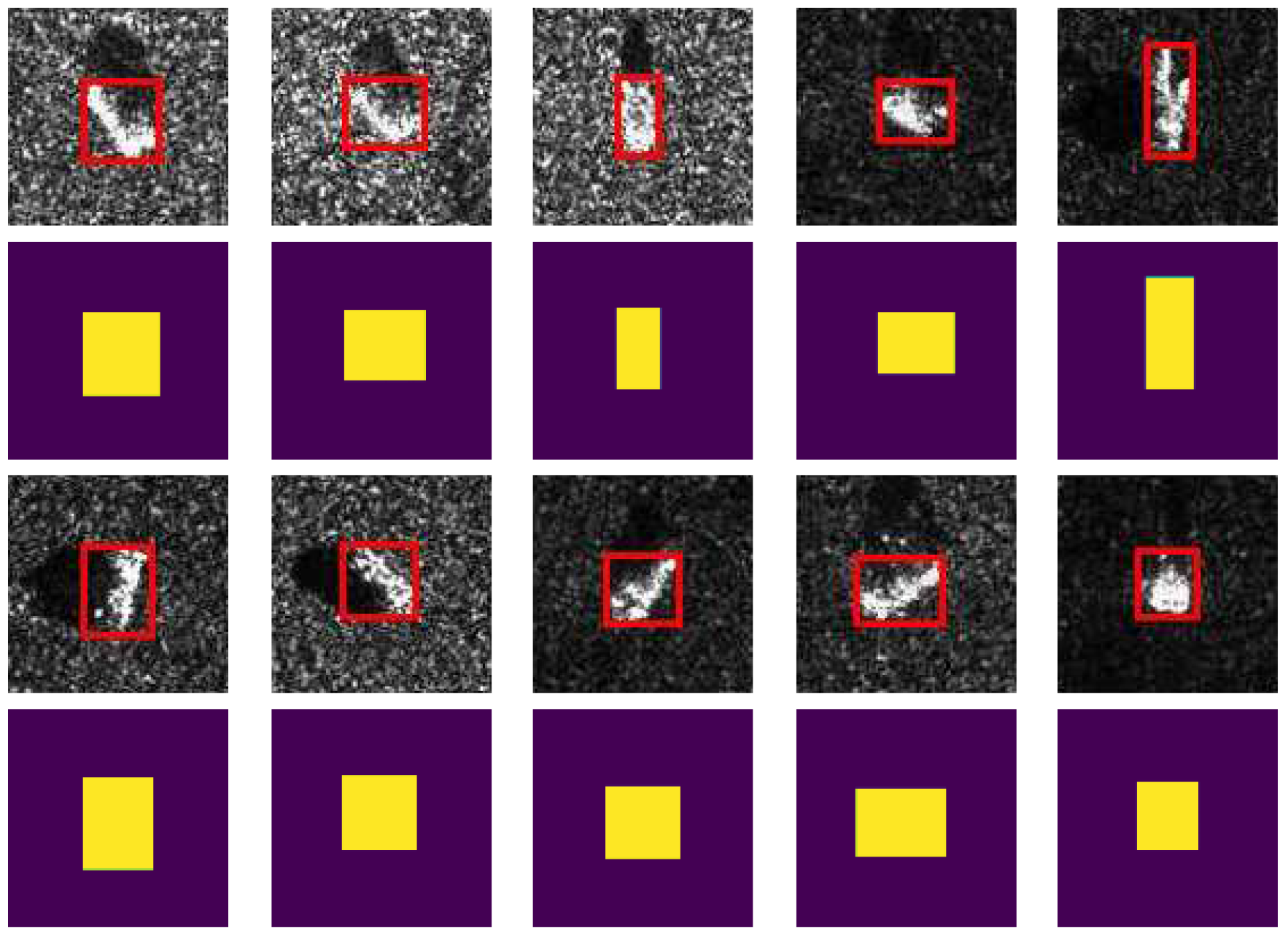
It is worth mentioning that the information contained in each image in the MSTAR dataset is a single target. And in different pictures, the position occupied by the target is usually a large area of the image, which facilitates us to label each subset.
Figure 8 shows the binarization results of ten groups of data randomly selected. We calculate
of images in each category of the testset separately, and the results are shown in
Table 1.
4.3. Conservation and Occlusion Test
In this section, we use the occlusion and conservation test [
36,
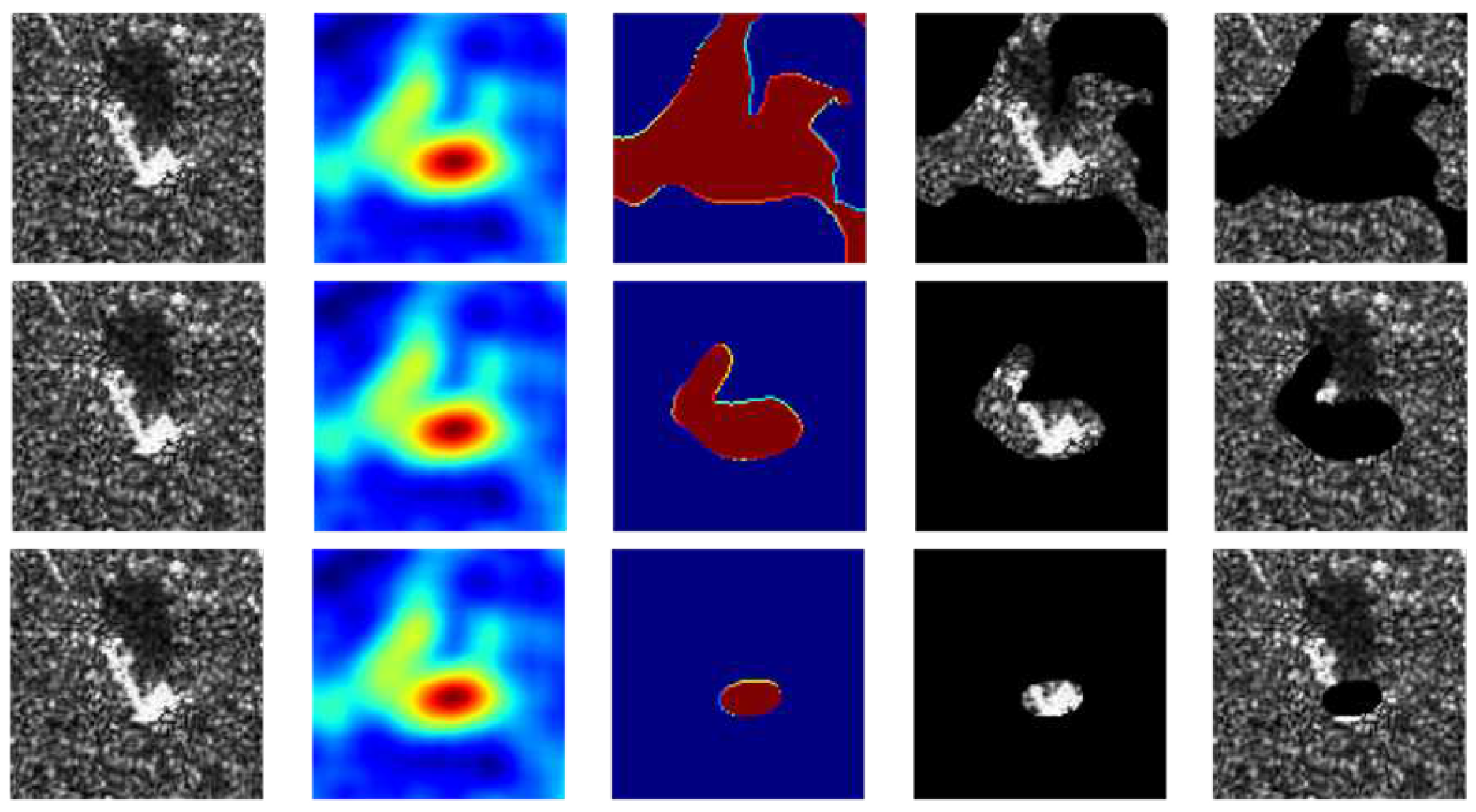
42] to analyze the localization capability of different methods quantitatively. The Conservation and Occlusion tests represent experiments in which only part of the area is preserved or abandoned, respectively. The experiments measures the effectiveness of the energy-concentrated regions in heatmaps by inputting the mask/reverse mask processed images into the black-box model and observing the change in scores, and the masks/reverse masks the resulting map obtained by binarization of the heatmap at different thresholds. The way masks generated is shown as Equations (
23) and (
24).
where
,
denotes the pixel value of the heatmap from C-RISE.
and
mean the masks/reverse masks, respectively.
Based on Equation (
23) and (
24), we could use the element-wise product to get the processed images
I/
after masked/reverse masked and the results after masked/reverse masked are shown in
Figure 9.
However, directly replacing some pixels with black may produce high-frequency sharp edges [
43], and these artificial traces may also lead to changes in the prediction probability, which cannot guarantee the fairness and objectivity of the model recognition process. In order to solve the above problems, we improved the original experiment and proposed two new measures, namely, introducing multiplicative noise and Gaussian blur to the occluded region. The follow two experiments show the effectiveness and rationality of our algorithm.
4.3.1. Based on Multiplicative Noise
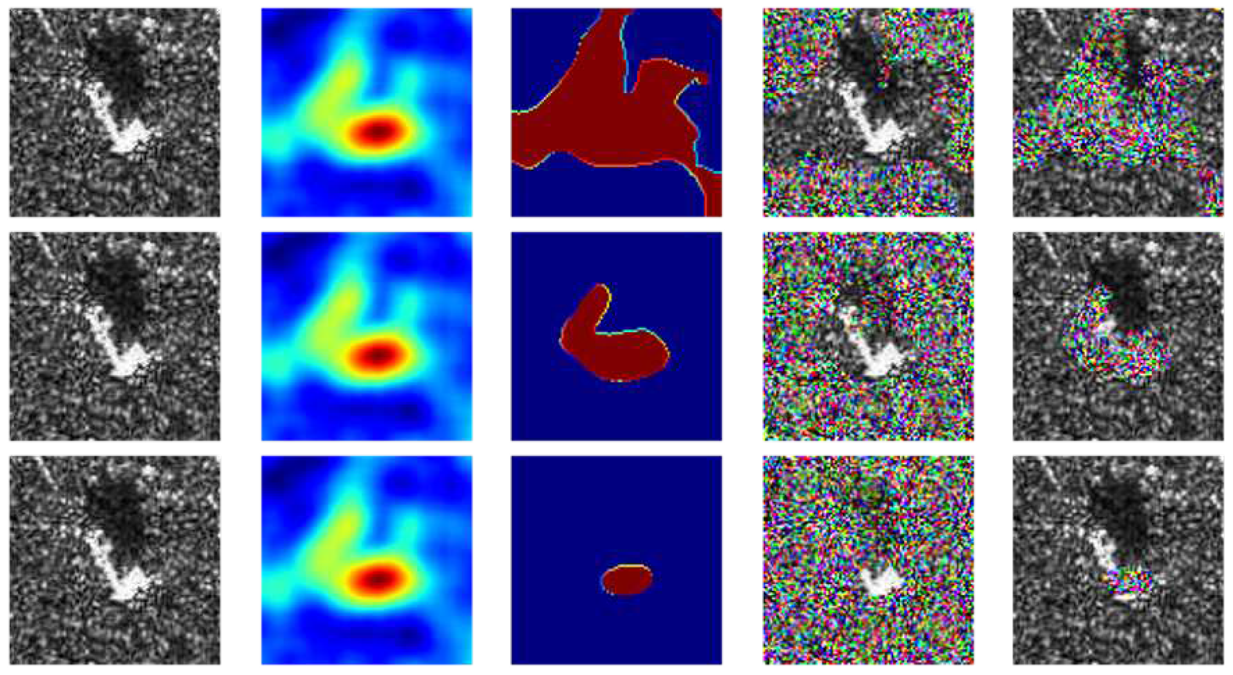
In the experiments, we firstly add multiplicative noise to the occluded region and updated Equations (
23) and (
24) to Equations (
27) and (
28). The reason for adding multiplicative noise is based on the physical scattering mechanism of SAR coherent imaging. We believe that the intensity of each resolved element of SAR image is modulated by the Radar Cross Section (RCS) [
3] of the ground object in the element and a multiplicative noise whose intensity follows the exponential distribution of unit mean (mean = 1). So we can consider the SAR image as the product of the RCS of the ground object in the scene and the noise of the unit mean exponential intensity distribution. Therefore, in the process of signal processing, we generally consider the noise of SAR image as multiplicative noise [
3,
6].
Figure 10 shows the above processing of the same image.
where
denotes add high-variance Gaussian multiplicative noise to the input image
X.
Then we define
to represent the divergence in the confidence that the processed image b and the original image a are classified into the same category. The mathematical expression of
is shown in Equation (
29).
where
is used to represent the score of the input image
x being classified as class
c. Based on this, we use
and
to represent the scores in the conservation and occlusion test, respectively. The process is shown as Equations (
30) and (
31).
It is worth noting that the smaller , the greater the difference between the values of and , and the generated heatmap can be considered to be located in the salient feature part of the target. Similarly, the larger the , the lager the difference between the values of and , and the main features after image processing can be considered to be preserved.
The
and
of various methods under different thresholds including Grad-CAM, Grad-CAM++, XGrad-CAM, Score-CAM, RISE and C-RISE, are shown in
Table 2 and
Table 3.
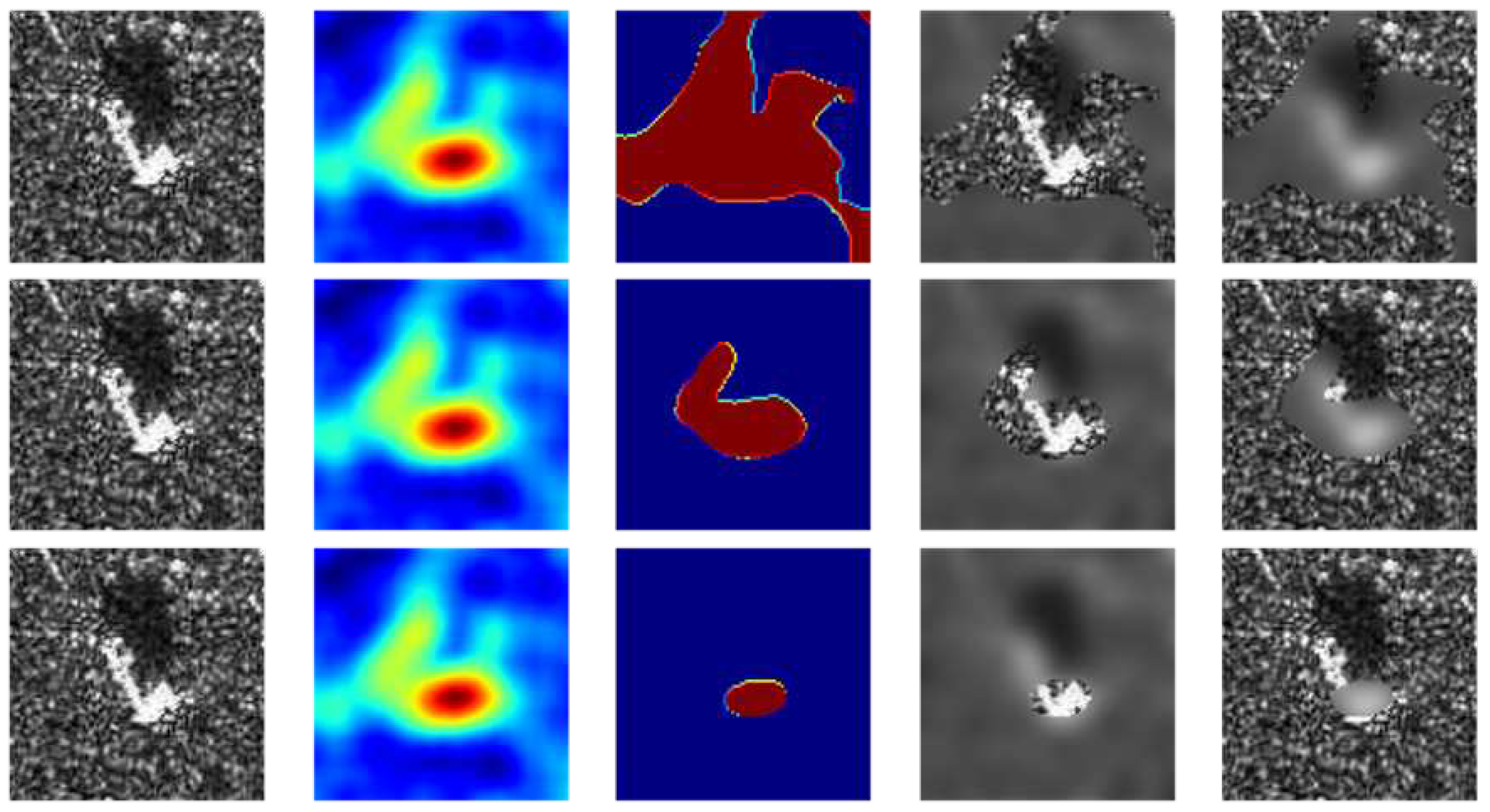
4.3.2. Based on Gaussian Blur
From
Table 2 and
Table 3, we can see that compared with other methods, C-RISE achieved relatively optimal performance under different thresholds. Similarly, we can also use high-variance Gaussian blur to process the masked area, and the processed results are shown in
Figure 11. Experimental indicators are shown in
Table 4 and
Table 5 respectively. The mathematical expressions are updated from Equations (
23) and (
24) to Equations (
32) and (
33).
where
denotes introduce high-variance Gaussian blur to the input image
X.
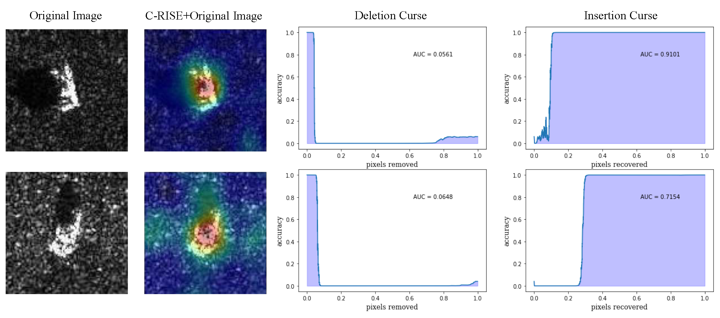
4.4. Insertion and Deletion Test
In this experiment, we compared different methods by insertion-deletion test [
41]. The experiment is a metric used to evaluate visual interpretation methods and measures the ability of visual interpretation to capture important pixels. During the deletion experiment, the
k most important pixels in the heatmap are successively removed, and then we calculate the degree of change in the prediction probability. The insertion curve is the opposite. The curves are shown in
Figure 12, with smaller
of deletion curves and higher
of insertion curves indicative of a better explanation. We randomly select an image from the test set for demonstration and plot its deletion and insertion curves of different algorithms. The results are shown in
Figure 13. We calculate
of both curves and the
score [
32] (
) of all images from the test set as a quantitative indicator. The average results over 2636 images is reported in
Table 6. We found that C-RISE achieves splendid results, indicating that the pixel importance revealed by the visualization method is in high agreement with the model and has great robustness.
5. Conclusions
This paper introduces C-RISE, a novel post-hoc interpretation method for black-box models in SAR ATR, which builds on the RISE algorithm. We compare the interpretation effects of different methods and C-RISE algorithm using both qualitative analysis and quantitative calculation. C-RISE offers several advantages, including its ability to group mask images that capture similar fusion features using a clustering strategy, which allows for concentration of more energy in the heatmap on the target area. Additionally, Gaussian blur is used to process the masked area, ensuring the consistency and integrity of the original image structure and taking into account both global and local characteristics. Compared with other neural network interpretable algorithms and even white box methods, C-RISE’s black-box model-oriented characteristics make it more robust and transferable. Furthermore, C-RISE avoids the error that can be caused by the unreasonable weight generation method in general CAM methods and the small feature map in the CNN model during the up-sampling process to the original image size. In our future work, we aim to explore the potential of C-RISE in identifying improper behaviors exhibited by black-box models and leveraging it to guide parameter adjustments. This will involve a systematic investigation of the capabilities of our proposed approach in identifying and diagnosing the sources of model inaccuracies and devising strategies to improve the performance of the black-box models. Such research endeavors will contribute to enhancing the interpretability and robustness of black-box models in various practical applications.
Author Contributions
Conceptualization, M.Z., J.C.,T.L.; methodology, J.C.; software, J.C., T.L.; validation, M.Z., T.L.; formal analysis,J.C., Z.F.; investigation, X.Z.; resources,M.Z., Y.L.; data curation,Y.L., Z.C.; writing—original draft preparation,J.C., Z.C.; writing—review and editing,M.Z., J.C. and T.L.; visualization, J.C. and Z.F.; supervision, X.Z.; project administration, M.Z. and X.Z.; funding acquisition, M.Z. and X.Z. All authors have read and agreed to the published version of the manuscript.
Funding
This research was funded by the Science and technology project of Xianyang city, grant number: 2021ZDZX-GY-0001.
Institutional Review Board Statement
Not applicable.
Informed Consent Statement
Not applicable
Data Availability Statement
In this paper, the SAR images of ten types of vehicle targets under standard operating conditions (SOC) in the MSTAR dataset are selected as experimental data. The dataset contains 5172 SAR images with the size of and the training set contains 2536 images, and 2636 are used for testing. These vehicle targets are: , , , , , , , , , . Readers can get the dataset from the author by email (agentcj@stu.xidian.edu.cn).
Acknowledgments
The authors would like to thank all the reviewers and editors for their great help and useful suggestions.
Conflicts of Interest
The authors declare no conflict of interest.
References
- Lin, M.; Chen,S.; Lu, F.; Xing, M.; Wei, J. Realizing Target Detection in SAR Images Based on Multiscale Superpixel Fusion. Sensors 2021, 21, 1643. [CrossRef]
- Wang, Z.; Wang, S.; Xu, C.; Li, C.; Yue, B.; Liang, X. SAR Images Super-resolution via Cartoon-texture Image Decomposition and Jointly Optimized Regressors. In Proceedings of the 2017 International Geoscience and Remote Sensing Symposium, Fort Worth, TX, USA, 23–28 July 2017; pp. 1668–1671. [CrossRef]
- Kong, L.; Xu, X. A MIMO-SAR Tomography Algorithm Based on Fully-Polarimetric Data. Sensors 2019, 19, 4839. [CrossRef]
- Novak, L.M.; Benitz, G.R.; Owirka, G.J.; Bessette, L.A. ATR performance using enhanced resolution SAR. Algorithms Synth. Aperture Radar Imag. III 1996, 2757, 332–337. [CrossRef]
- Ding, B.; Wen.G.; Huang, X.; Ma, C.; Yang, X. Data augmentation by multilevel reconstruction using attributed scattering center for SAR target recognition. IEEE Geosci. Remote Sens. Lett. 2017, 14, 979–983. [CrossRef]
- Ding, B.; Wen, G.; Huang, X.; Ma, C.; Yang, X. Data Augmentation by Multilevel Reconstruction Using Attributed Scattering Center for SAR Target Recognition. IEEE Geosci. Remote Sens. Lett. 2017, 14, 979–983. [CrossRef]
- Wang, Y.; Zhang, Y.; Qu, H.; Tian, Q. Target Detection and Recognition Based on Convolutional Neural Network for SAR Image. In Proceedings of the 2018 11th International Congress on Image and Signal Processing, Biomedical Engineering and Informatics, Beijing, China, 13–15 October 2018; pp. 1–5. [CrossRef]
- Mohsenzadegan, K.; Tavakkoli, V.; Kyamakya, K. A Deep-Learning Based Visual Sensing Concept for a Robust Classification of Document Images under Real-World Hard Conditions. Sensors 2021, 21, 6763. [CrossRef]
- LeCun, Y.; Bengio, Y.; Hinton, G. Deep learning. Nature 2015, 521, 436–444. [CrossRef]
- Dong, Y.P.; Su, H.; Wu, B.Y. Efficient Decision-based Black-box Adversarial Attacks on Face Recognition. In Proceedings of the 2019 IEEE/CVF Conference on Computer Vision and Pattern Recognition (CVPR), Long Beach, CA, USA, 15–20 June 2019. [CrossRef]
- Wang, Y.P.; Zhang, Y.B.; Qu, H.Q.; Tian, Q. Target Detection and Recognition Based on Convolutional Neural Network for SAR Image. In Proceedings of the 2018 11th International Congress on Image and Signal Processing, BioMedical Engineering and Informatics, Beijing, China, 13–15 October 2018. [CrossRef]
- Cai, J.L.; Jia, H.G.; Liu, G.X.; Zhang, B.; Liu, Q.; Fu, Y.; Wang, X.W.; Zhang, R. An Accurate Geocoding Method for GB-SAR Images Based on Solution Space Search and Its Application in Landslide Monitoring. Remote Sens. 2021, 13, 832. [CrossRef]
- Cho, J.H.; Park, C.G. Multiple Feature Aggregation Using Convolutional Neural Networks for SAR Image-Based Automatic Target Recognition. IEEE Geosci. Remote Sens. Lett. 2018, 56, 1882–1886. [CrossRef]
- LeCun Y, Bottou L, Bengio Y, et al. Gradient-based learning applied to document recognition. Proc. IEEE 1998, 86, 2278-2324. [CrossRef]
- Krizhevsky A, Sutskever I, Hinton G E. Imagenet classification with deep convolutional neural networks. Commun. ACM 2017, 60, 84-90.
- Szegedy C, Liu W, Jia Y, et al. Going deeper with convolutions. In Proceedings of the IEEE conference on computer vision and pattern recognition, 2015; pp. 1-9. [CrossRef]
- Simonyan K, Zisserman A. Very deep convolutional networks for large-scale image recognition. arXiv 2014, arXiv:1409.1556. [CrossRef]
- He K, Zhang X, Ren S, et al. Deep residual learning for image recognition. In Proceedings of the IEEE conference on computer vision and pattern recognition, 2016; pp. 770-778. [CrossRef]
- Dong, Y.P.; Su, H.; Wu, B.Y. Efficient Decision-based Black-box Adversarial Attacks on Face Recognition. In Proceedings of the 2019 IEEE/CVF Conference on Computer Vision and Pattern Recognition (CVPR), Long Beach, CA, USA, 15–20 June 2019. [CrossRef]
- Giacalone, J.; Bourgeois, L.; Ancora, A. Challenges in aggregation of heterogeneous sensors for Autonomous Driving Systems. In Proceedings of the 2019 IEEE Sensors Applications Symposium, Sophia Antipolis, France, 11–13 March 2019; pp. 1–5. [CrossRef]
- Hinton G E, Srivastava N, Krizhevsky A, et al. Improving neural networks by preventing co-adaptation of feature detectors. arXiv 2012, arXiv:1207.0580. [CrossRef]
- Montavon, G.; Binder, A.; Lapuschkin, S.; Samek, W.; Müller, K.R. Layer-Wise Relevance Propagation: An Overview. In Explainable AI: Interpreting, Explaining and Visualizing Deep Learning; Samek, W., Montavon, G., Vedaldi, A., Hansen, L., Müller, K.R., Eds.; Springer: Cham, Switzerland, 2019; pp. 14–15.
- Zhu, C.; Chen, Z.; Zhao, R.; Wang, J.; Yan, R. Decoupled Feature-Temporal CNN: Explaining Deep Learning-Based MachineHealth Monitoring. IEEE Trans. Instrum. Meas. 2021, 70, 1–13.
- Saurabh, D.; Harish, G.R. Ablation-CAM: Visual Explanations for Deep Convolutional Network via Gradient-free Localization. In Proceedings of the 2020 IEEE Winter Conference on Applications of Computer Vision (WACV), Snowmass, CO, USA,1–5 March 2020. [CrossRef]
- Simonyan K, Vedaldi A, Zisserman A. Deep inside convolutional networks: Visualising image classification models and saliency maps[C]. In 2nd International Conference on Learning Representations, Banff, AB, Canada, 2014.
- Zeiler M D, Fergus R. Visualizing and understanding convolutional networks. In Proceedings of the 13th European Conference on Computer Vision, Zurich, Switzerland, 2014; pp. 818– 833.
- Sundararajan M, Taly A, Yan Q. Axiomatic attribution for deep networks[C]. Proceedings of the 34th International Conference on Machine Learning, Sydney, NSW, Australia, 2017; pp. 3319–3328.
- Smilkov D, Thorat N, Kim B, et al. Smooth-grad: Removing noise by adding noise. CoRR 2017, abs/1706.03825.
- Springenberg J T, Dosovitskiy A, Brox T, et al. Striving for simplicity: The all convolutional net[C]. In 3rd International Conference on Learning Representations, San Diego, CA, USA, 2015.
- Srinivas S, Fleuret F. Full-gradient representation for neural network visualization[C]. Advances in Neural Information Processing Systems, Vancouver, BC, Canada, 2019; pp. 4126– 4135.
- Bach S, Binder A, Montavon G, et al. On pixel-wise explanations for non-linear classifier decisions by layer-wise relevance propagation. PLoS ONE 2015, 10, 1 – 46. [CrossRef]
- Zhang Q, Rao L, Yang Y. Group-cam: Group score-weighted visual explanations for deep convolutional networks. arXiv 2021 arXiv:2103.13859. [CrossRef]
- Zhou, B.; Khosla, K.; Lapedriza, A.; Oliva, A.; Torralba, A. Learning Deep Features for Discriminative Localization. In Proceedings of the 2016 IEEE/CVF Conference on Computer Vision and Pattern Recognition (CVPR), Las Vegas, NV, 26 June–1 July 2016. [CrossRef]
- Ramprasaath, R.S.; Michael, C.; Abhishek, D. Grad-CAM: Visual Explanations from Deep Networks via Gradient-based Localization. arXiv 2015, arXiv:1610.02391v4. [CrossRef]
- Aditya, C.; Anirban, S.; Abhishek, D.; Prantik H. Grad-CAM++: Improved Visual Explanations for Deep Convolutional Networks. arXiv 2018, arXiv:1710.11063v34. [CrossRef]
- Fu, H.G.; Hu, Q.Y.; Dong, X.H.; Guo, Y.I.; Gao, Y.H.; Li, B. Axiom-based Grad-CAM: Towards Accurate Visualization and Explanation of CNNs. In Proceedings of the 2020 31th British Machine Vision Conference (BMVC), Manchester, UK, 7–10 September 2020.
- Wang, H.F.; Wang, Z.F.; Du, M.N. Methods for Interpreting and Understanding Deep Neural Networks. In Proceedings of the 2020 IEEE/CVF Conference on Computer Vision and Pattern Recognition Workshops (CVPRW), Seattle, WA, USA, 14–19 June 2020.
- Fong R, Vedaldi A. Interpretable explanations of black boxes by meaningful perturbation[C]. In IEEE International Conference on Computer Vision, Venice, Italy, 2017: 3449– 3457. [CrossRef]
- Fong R, Patrick M, Vedaldi A. Understanding deep networks via extremal perturbations and smooth masks[C]. In IEEE International Conference on Computer Vision, Seoul, Korea, 2019: 2950– 2958. [CrossRef]
- Ribeiro, M.; Singh, S.; Guestrin, C. “Why Should I Trust You?”: Explaining the Predictions of Any Classifier. Assoc. Comput. Mach. 2016, 1135–1144. [CrossRef]
- Petsiuk V, Das A, Saenko K. RISE: Randomized input sampling for explanation of black-box model. In Proceedings of the British Machine Vision Conference, Newcastle, UK, 2018: 151– 168.
- Wissinger, J.; Ristroph, R.; Diemunsch, J.R.; Severson, W.E.; Fruedenthal, E. MSTAR’s extensible search engine and model-based inferencing toolkit. In Proceedings of the Algorithms for Synthetic Aperture Radar Imagery VI, Orlando, FL, USA, 5–9 April 1999; Volume 3721, pp. 554–570. [CrossRef]
- Novak, L.M.; Benitz, G.R.; Owirka, G.J.; Bessette, L.A. ATR performance using enhanced resolution SAR.Algorithms Synth. Aperture Radar Imag. III 1996, 2757, 332–337. [CrossRef]
- Dong, Y.P.; Su, H.;Wu, B.Y. Efficient Decision-based Black-box Adversarial Attacks on Face Recognition. In Proceedings of the 2019 IEEE/CVF Conference on Computer Vision and Pattern Recognition (CVPR), Long Beach, CA, USA, 15–20 June 2019. [CrossRef]
Figure 1.
The flowchart of RISE method.
Figure 1.
The flowchart of RISE method.
Figure 2.
The flowchart of C-RISE.
Figure 2.
The flowchart of C-RISE.
Figure 3.
The flowchart of generating masks.
Figure 3.
The flowchart of generating masks.
Figure 4.
10 typical SAR images for each category in MSTAR. The first row depicting random images from , , , , and , and the second row showing randomly selected images from , , , and .
Figure 4.
10 typical SAR images for each category in MSTAR. The first row depicting random images from , , , , and , and the second row showing randomly selected images from , , , and .
Figure 5.
The structure of Alexnet.
Figure 5.
The structure of Alexnet.
Figure 6.
Comparison of Grad-CAM, Grad-CAM++, XGrad-CAM, Score-CAM, RISE, C-RISE. The first column is the SAR images of ten classes. The rest of columns are corresponding heatmaps generated by each method respectively.
Figure 6.
Comparison of Grad-CAM, Grad-CAM++, XGrad-CAM, Score-CAM, RISE, C-RISE. The first column is the SAR images of ten classes. The rest of columns are corresponding heatmaps generated by each method respectively.
Figure 7.
The flowchat of calculating .
Figure 7.
The flowchat of calculating .
Figure 8.
The first and third rows represent randomly selected images with bounding boxes from 10 categories in the test set and the results of binarization of each images are shown as the second and fourth rows.
Figure 8.
The first and third rows represent randomly selected images with bounding boxes from 10 categories in the test set and the results of binarization of each images are shown as the second and fourth rows.
Figure 9.
The first column represents a randomly selected image from , the second column represents , the third column represents , and the fourth and fifth columns represent images after masked/reverse masked, respectively. The selected in the three lines were , and , respectively.
Figure 9.
The first column represents a randomly selected image from , the second column represents , the third column represents , and the fourth and fifth columns represent images after masked/reverse masked, respectively. The selected in the three lines were , and , respectively.
Figure 10.
The first column represents a randomly selected image from , the second column represents , the third column represents , and the fourth and fifth columns represent images after masked/reverse masked based on multiplicative noise, respectively. The selected in the three lines were , and , respectively.
Figure 11.
The first column represents a randomly selected image from , the second column represents , the third column represents , and the fourth and fifth columns represent images after masked/reverse masked based on Gaussian blur, respectively. The selected in the three lines were , and , respectively.
Figure 12.
The heatmap generated by C-RISE (second column) for two representative images (first column) with deletion (third column) and insertion (fourth column) curves.
Figure 12.
The heatmap generated by C-RISE (second column) for two representative images (first column) with deletion (third column) and insertion (fourth column) curves.
Figure 13.
Grad-CAM, Grad-CAM++, XGrad-CAM, Score-CAM, RISE and C-RISE generated saliency maps for a seleted image randomly(firstly column) in terms of deletion (second column) and insertion curves (third column).
Figure 13.
Grad-CAM, Grad-CAM++, XGrad-CAM, Score-CAM, RISE and C-RISE generated saliency maps for a seleted image randomly(firstly column) in terms of deletion (second column) and insertion curves (third column).
Table 1.
The of images in each category. The best records are marked in bold.
Table 1.
The of images in each category. The best records are marked in bold.
| |
Grad-CAM |
Grad-CAM++ |
XGrad-CAM |
Score-CAM |
RISE |
C-RISE |
| 2S1 |
0.5764 |
0.4252 |
0.5785 |
0.5524 |
0.3483 |
0.5876 |
| BRDM_2 |
0.5881 |
0.5138 |
0.5970 |
0.6230 |
0.3621 |
0.5930 |
| BTR_60 |
0.4355 |
0.3744 |
0.4553 |
0.3892 |
0.1024 |
0.4731 |
| D7 |
0.3782 |
0.6225 |
0.3920 |
0.5425 |
0.6406 |
0.4394 |
| SN_132 |
0.3820 |
0.5579 |
0.4168 |
0.4915 |
0.4797 |
0.4723 |
| SN_9563 |
0.4895 |
0.4024 |
0.4851 |
0.4421 |
0.2964 |
0.4817 |
| SN_C71 |
0.4121 |
0.2868 |
0.4409 |
0.3823 |
0.0856 |
0.4494 |
| T62 |
0.4975 |
0.3894 |
0.5158 |
0.4886 |
0.3374 |
0.5233 |
| ZIL131 |
0.5420 |
0.3984 |
0.5559 |
0.5265 |
0.4254 |
0.5498 |
| ZSU_23_4 |
0.4018 |
0.5315 |
0.4298 |
0.4616 |
0.5209 |
0.4474 |
| average |
0.4758 |
0.4555 |
0.4918 |
0.4976 |
0.3726 |
0.5060 |
Table 2.
of Different Methods in Conservation and Occlusion Test Based on Multiplicative Noise.The best records are marked in bold.
Table 2.
of Different Methods in Conservation and Occlusion Test Based on Multiplicative Noise.The best records are marked in bold.
| threshold |
Grad-CAM |
Grad-CAM++ |
XGrad-CAM |
Score-CAM |
RISE |
C-RISE |
| 0.25 |
0.6975 |
0.6731 |
0.6949 |
0.7017 |
0.7364 |
0.6672 |
| 0.50 |
0.6750 |
0.7063 |
0.6760 |
0.6776 |
0.8257 |
0.6658 |
| 0.75 |
0.7620 |
0.7691 |
0.7644 |
0.7615 |
0.7646 |
0.6626 |
Table 3.
of Different Methods in Conservation and Occlusion Test Based on Multiplicative Noise. The best records are marked in bold.
Table 3.
of Different Methods in Conservation and Occlusion Test Based on Multiplicative Noise. The best records are marked in bold.
| threshold |
Grad-CAM |
Grad-CAM++ |
XGrad-CAM |
Score-CAM |
RISE |
C-RISE |
| 0.25 |
0.7008 |
0.6434 |
0.6973 |
0.6427 |
0.4372 |
0.4934 |
| 0.50 |
0.3524 |
0.3287 |
0.4791 |
0.4804 |
0.1867 |
0.5361 |
| 0.75 |
0.1306 |
0.0475 |
0.1026 |
0.1359 |
0.1537 |
0.2637 |
Table 4.
of Different Methods in Conservation and Occlusion Test Based on Gaussian blur.The best records are marked in bold.
Table 4.
of Different Methods in Conservation and Occlusion Test Based on Gaussian blur.The best records are marked in bold.
| threshold |
Grad-CAM |
Grad-CAM++ |
XGrad-CAM |
Score-CAM |
RISE |
C-RISE |
| 0.25 |
0.0665 |
0.1038 |
0.0768 |
0.0205 |
0.0137 |
0.0064 |
| 0.50 |
0.0285 |
0.2391 |
0.1764 |
0.0944 |
0.0924 |
0.1692 |
| 0.75 |
0.3147 |
0.3721 |
0.3249 |
0.2893 |
0.2466 |
0.1631 |
Table 5.
of Different Methods in Conservation and Occlusion Test Based on Multiplicative Noise. The best records are marked in bold.
Table 5.
of Different Methods in Conservation and Occlusion Test Based on Multiplicative Noise. The best records are marked in bold.
| threshold |
Grad-CAM |
Grad-CAM++ |
XGrad-CAM |
Score-CAM |
RISE |
C-RISE |
| 0.25 |
0.2805 |
0.2250 |
0.2682 |
0.3283 |
0.3898 |
0.3985 |
| 0.50 |
0.1634 |
0.0968 |
0.1519 |
0.2217 |
0.2513 |
0.2870 |
| 0.75 |
0.0350 |
0.0119 |
0.0305 |
0.0556 |
0.0906 |
0.1663 |
Table 6.
Comparative evaluation in terms of deletion (lower is better) and insertion (higher AUC is better) .The score (higher is better) shows that C-RISE outperform other related methods significantly. The best records are marked in bold.
Table 6.
Comparative evaluation in terms of deletion (lower is better) and insertion (higher AUC is better) .The score (higher is better) shows that C-RISE outperform other related methods significantly. The best records are marked in bold.
|
Grad-CAM |
Grad-CAM++ |
XGrad-CAM |
Score-CAM |
RISE |
C-RISE |
| Insertion |
0.2768 |
0.3011 |
0.4145 |
0.5512 |
0.4659 |
0.6875 |
| Deletion |
0.1317 |
0.1676 |
0.1255 |
0.0246 |
0.0420 |
0.1317 |
| over_all |
0.1451 |
0.1335 |
0.2890 |
0.5266 |
0.4239 |
0.5558 |
|
Disclaimer/Publisher’s Note: The statements, opinions and data contained in all publications are solely those of the individual author(s) and contributor(s) and not of MDPI and/or the editor(s). MDPI and/or the editor(s) disclaim responsibility for any injury to people or property resulting from any ideas, methods, instructions or products referred to in the content. |
© 2023 by the authors. Licensee MDPI, Basel, Switzerland. This article is an open access article distributed under the terms and conditions of the Creative Commons Attribution (CC BY) license (http://creativecommons.org/licenses/by/4.0/).
