Submitted:
21 April 2023
Posted:
23 April 2023
You are already at the latest version
Abstract
Keywords:
1. Introduction
- We develop a multi-objective node selection optimization model that takes into account accuracy, robustness, and latency simultaneously.
- We formulate the multi-objective node selection as a Markov decision process(MDP), defining the state space, action space, and reward function.
- Based on the multi-objective and deep reinforcement learning, we design a DQN-based algorithm to solve the node selection problem.
2. Related Work
3. System Model
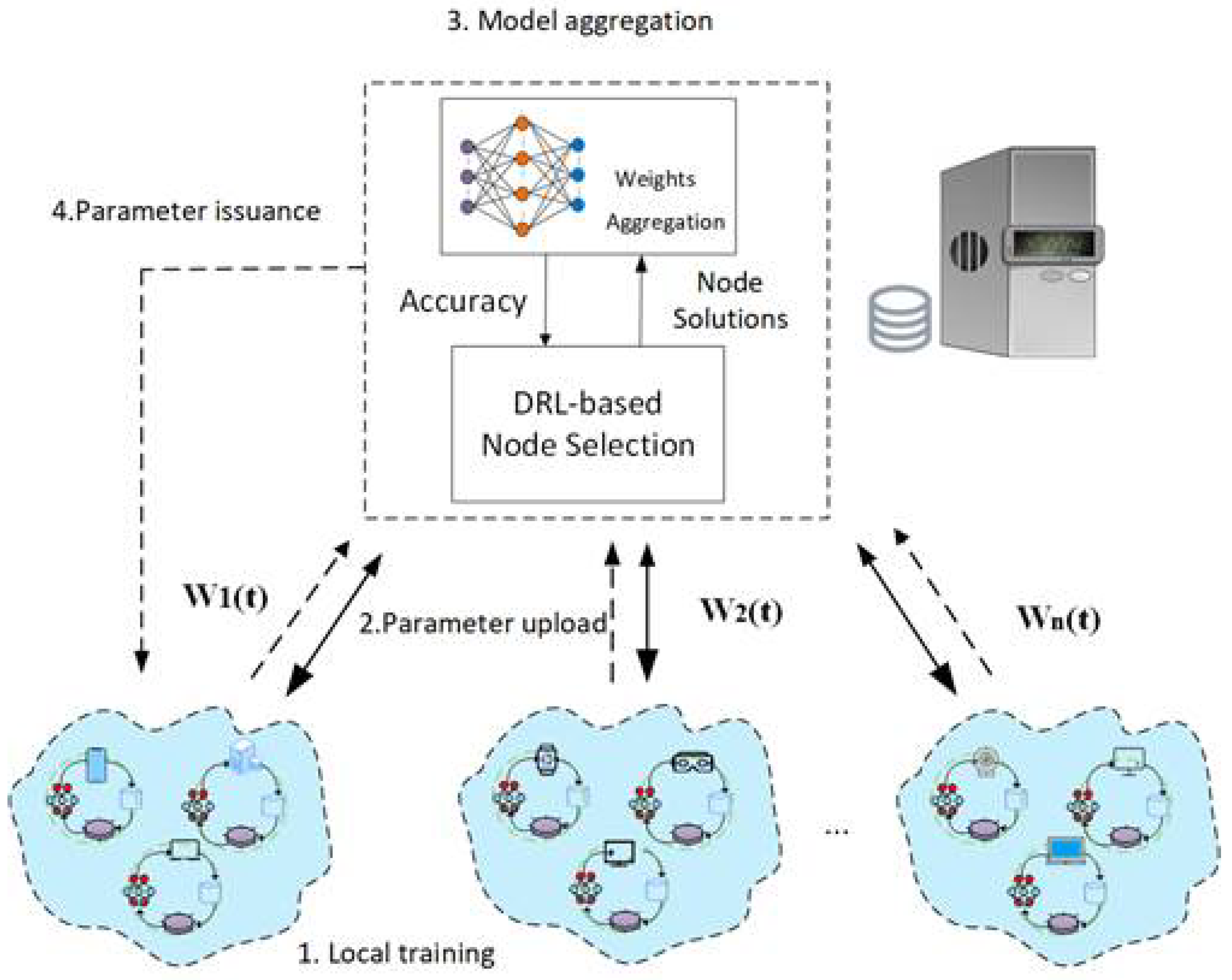
3.1. Network Model
| parameters | Meaning |
| The data set of terminal d participating in federal learning | |
| Total data set related to FL task i | |
| The size of the dataset for terminal d participates in FL tasks. | |
| The size of the total data set for this federal learning task | |
| Collection of attributes for FL task i | |
| The number of CPU cycles required for calculating a set of data in dataset | |
| Initial model of FL task i | |
| Loss function of device d when performing local training of FL task i | |
| The model parameters of device d at the nth training session | |
| Learning rate d of device when performing local training of FL task i | |
| Sum of loss functions for the FL task i test dataset | |
| The local computation time of FL task i | |
| The transmission time of FL task i | |
| The CPU cycle frequency of device d in executing FL task i | |
| The transfer rate of task i in FL between the device and the server. | |
| G | The number of CPU cycles required per data for device in the FL task i |
| The environmental state at time t | |
| The dataset of terminal at the previous time step | |
| The action space at time t | |
| Whether device d is selected to participate in FL task i | |
| The max delay of clients participating in this iteration | |
| A policy is a mapping from a state space to an action space | |
| Discount factor |
3.2. Workflow for Federated Learning Training
3.3. Problem Formulation for Node Selection
4. FL node selection algorithm based on DQN
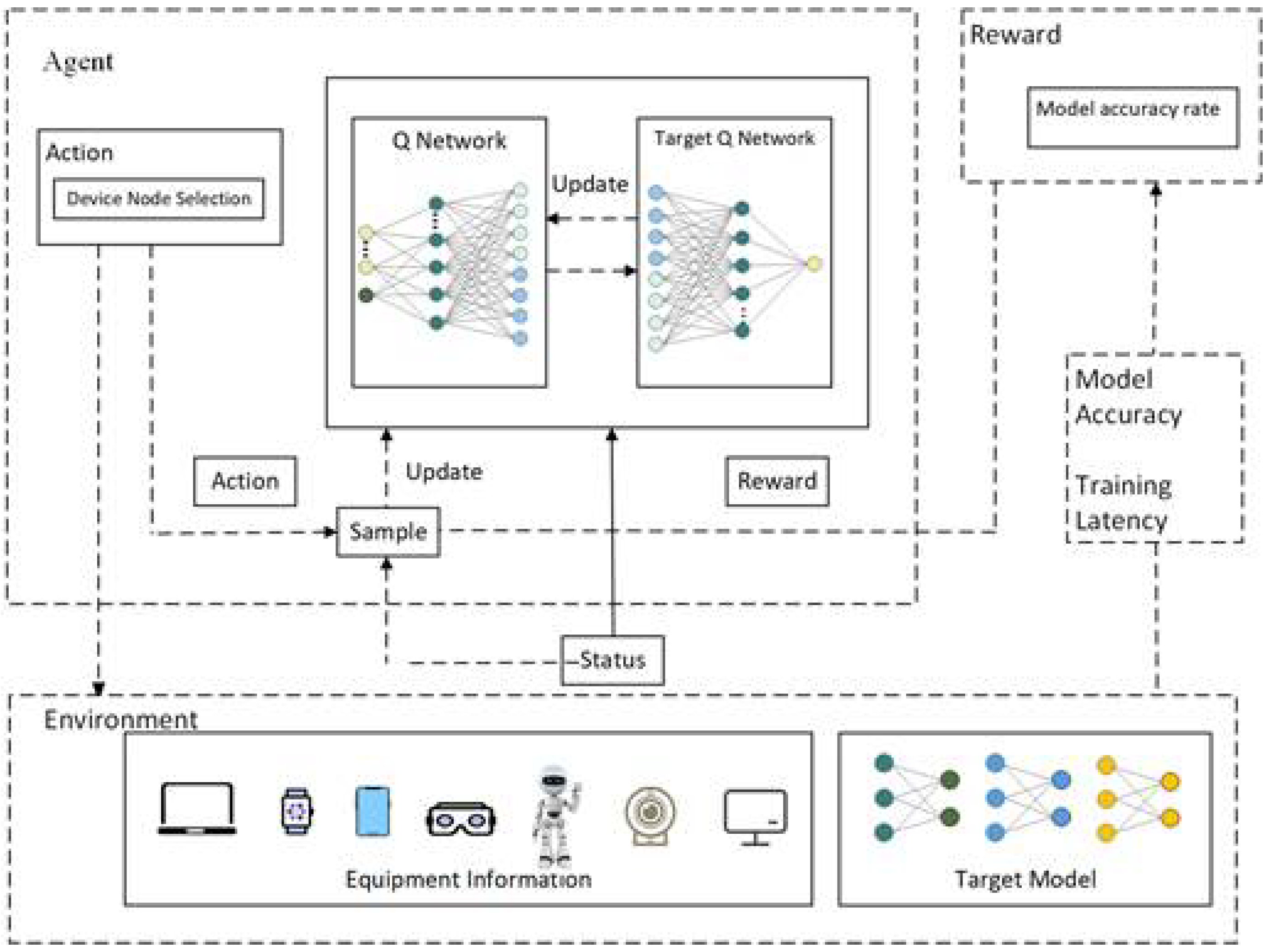
4.1. MDP Model
4.1.1. State Space
4.1.2. Action Space
4.1.3. Reward Function
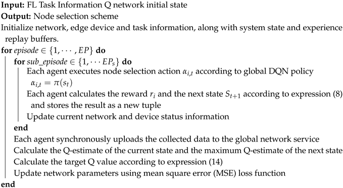
4.2. DQN-Based Algorithm for FL Node Selection
| Algorithm 1: DQN-based node selection algorithm |
 |
5. Simulation Analysis
5.1. Experimental Settings
| Parameter Type | Parameter | Parameter Description | Parameter Value |
| Equipment and model parameters | Number of terminals | 100 | |
| CPU cycle frequency | [0,1] | ||
| Wireless Bandwidth | [0,2] | ||
| Eocal data sets | 600 | ||
| Local Iteration | 2 | ||
| Minimum sample size | 10 | ||
| Learning Rate | 0.01 | ||
| Node | Number of nodes involved | [10,80] | |
| Number of CPU cycles required for | 7000 | ||
| training per data bit | |||
| Global Model Size | 20Mbit | ||
| DQN parament | A | Agents | 4 |
| s | Training steps | 1000 | |
| Target Q | Q Network | 0.0001 | |
| Bonus Discount Factor | 0.9 | ||
| circle | Strategy Update Steps | 100 | |
| Experience replay buffer | 10000 | ||
| B | Batch-size | 64 |
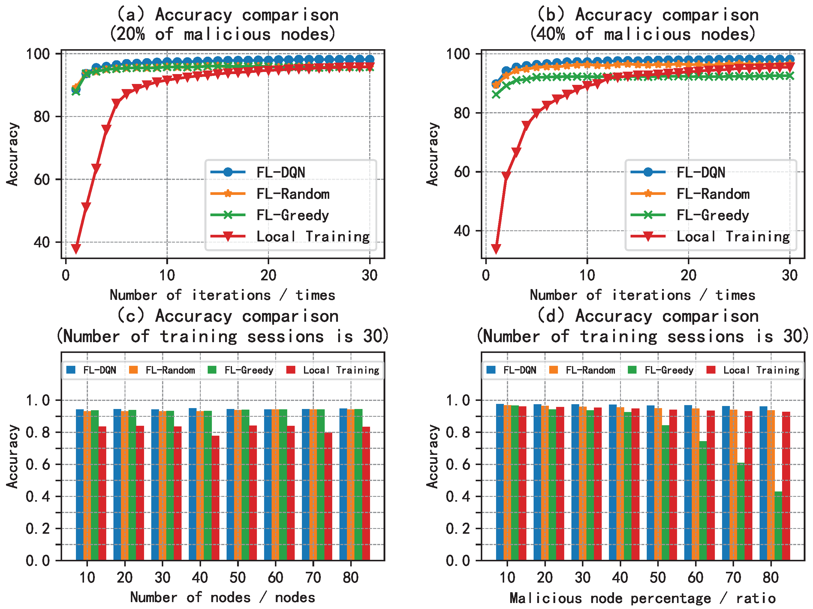
5.2. Analysis of Results
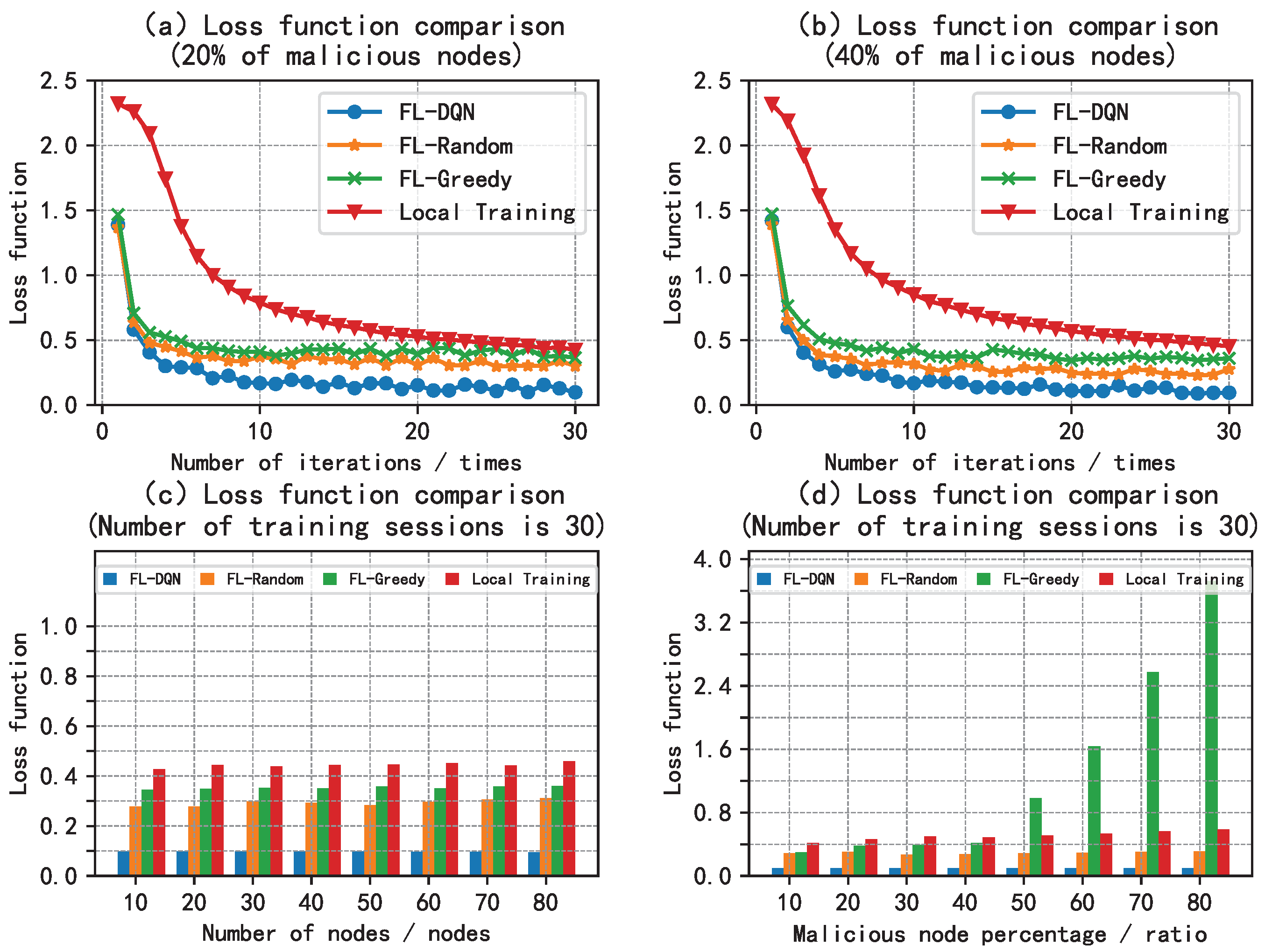
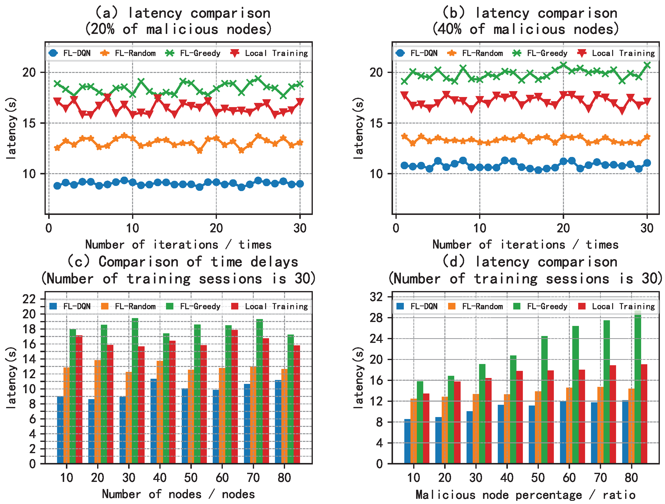
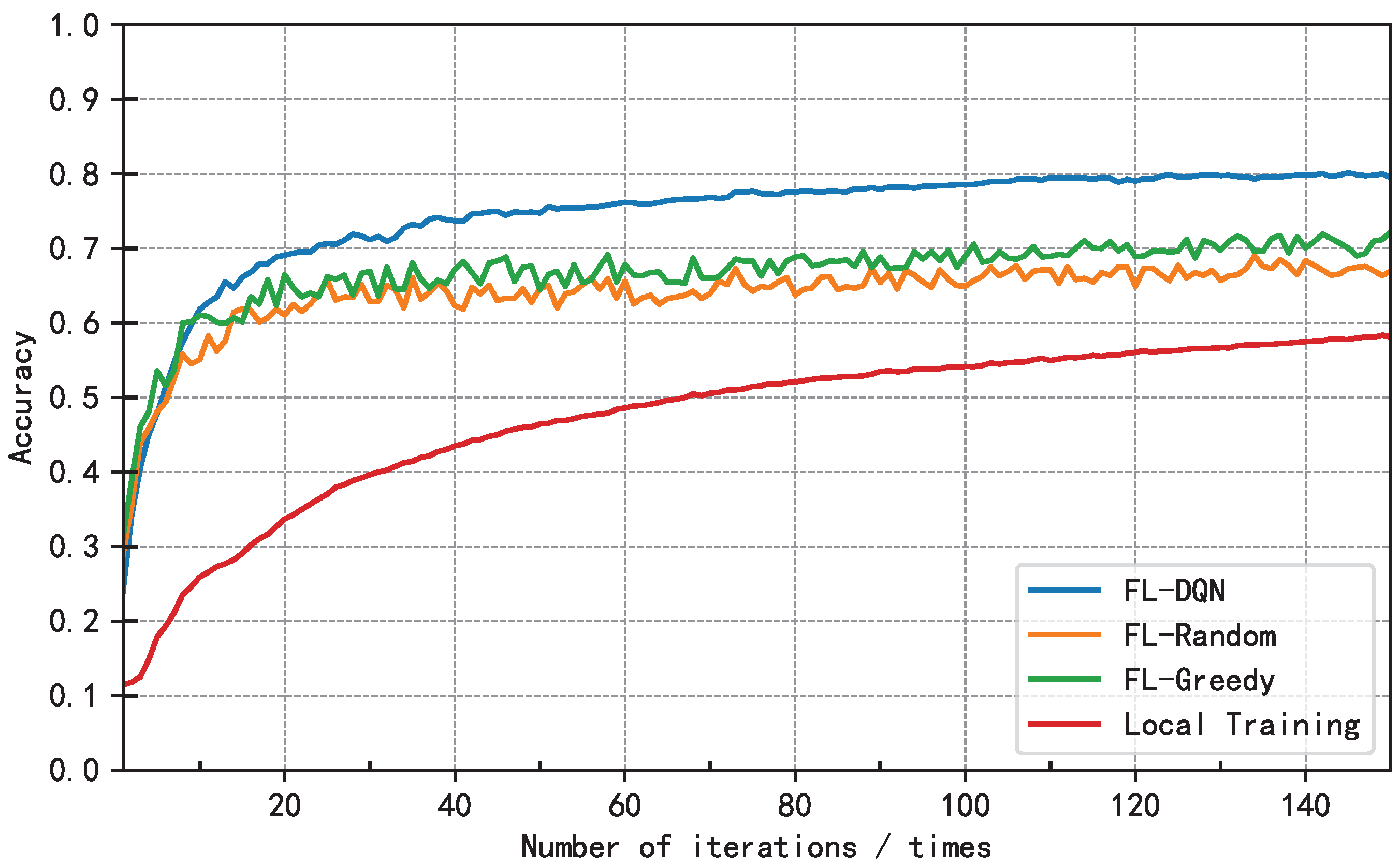
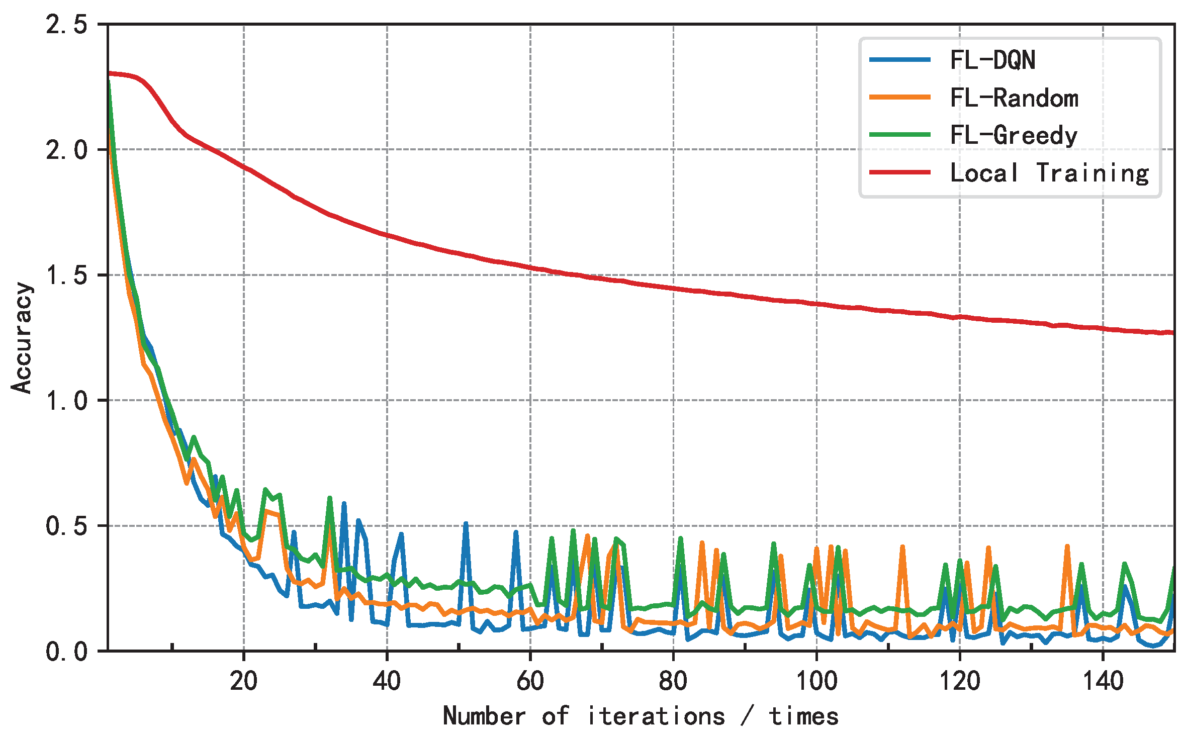
6. Conclusion
References
- McMahan B, Moore E, Ramage D, et al. Communication-efficient learning of deep networks from decentralized data [c]//Artificial intelligence and statistics. PMLR, 2017: 1273-1282.
- Kairouz P, McMahan H B, Avent B, et al. Advances and open problems in federated learning [J] Foundations and Trends® in Machine Learning, 2021, 14(1–2): 1-210.
- Nguyen D C, Cheng P, Ding M, et al. Enabling AI in future wireless networks: A data life cycle perspective [J] IEEE Communications Surveys & Tutorials, 2020, 23(1): 553-595.
- Mora A, Fantini D, Bellavista P. Federated Learning Algorithms with Heterogeneous Data Distributions: An Empirical Evaluation [c]//2022 IEEE/ACM 7th Symposium on Edge Computing (SEC). IEEE, 2022: 336-341.
- Chathoth A K, Necciai C P, Jagannatha A, et al. Differentially Private Federated Continual Learning with Heterogeneous Cohort Privacy [c]//2022 IEEE International Conference on Big Data (Big Data). IEEE, 2022: 5682-5691.
- Xia W, Quek T Q S, Guo K, et al. Multi-armed bandit-based client scheduling for federated learning [J] IEEE Transactions on Wireless Communications, 2020, 19(11): 7108-7123.
- Deer A, Ali R E, Avestimehr A S. On Multi-Round Privacy in Federated Learning [c]//2022 56th Asilomar Conference on Signals, Systems, and Computers. IEEE, 2022: 764-769.
- Liu W, Chen L, Zhang W. Decentralized federated learning: Balancing communication and computing costs [J] IEEE Transactions on Signal and Information Processing over Networks, 2022, 8: 131-143.
- Lu Y, Huang X, Zhang K, et al. Blockchain empowered asynchronous federated learning for secure data sharing in internet of vehicles [J] IEEE Transactions on Vehicular Technology, 2020, 69(4): 4298-4311.
- Chi J, Xu S, Guo S, et al. Federated Learning Empowered Edge Collaborative Content Caching Mechanism for Internet of Vehicles [c]//NOMS 2022-2022 IEEE/IFIP Network Operations and Management Symposium. IEEE, 2022: 1-5.
- Xu J, Glicksberg B S, Su C, et al. Federated learning for healthcare informatics [J] Journal of Healthcare Informatics Research, 2021, 5: 1-19.
- Moon S H, Lee W H. Privacy-Preserving Federated Learning in Healthcare [c]//2023 International Conference on Electronics, Information, and Communication (ICEIC). IEEE, 2023: 1-4.
- Vrind T, Pathak L, Das D. Novel Federated Learning by Aerial-Assisted Protocol for Efficiency Enhancement in Beyond 5G Network [c]//2023 IEEE 20th Consumer Communications & Networking Conference (CCNC). IEEE, 2023: 891-892.
- Zhang H, Zhou H, Erol-Kantarci M. Federated deep reinforcement learning for resource allocation in O-RAN slicing [c]//GLOBECOM 2022-2022 IEEE Global Communications Conference. IEEE, 2022: 958-963.
- Guo X. Implementation of a Blockchain-enabled Federated Learning Model that Supports Security and Privacy Comparisons [c]//2022 IEEE 5th International Conference on Information Systems and Computer Aided Education (ICISCAE). IEEE, 2022: 243-247.
- Xin S, Zhuo L, Xin C. Node Selection Strategy Design Based on Reputation Mechanism for Hierarchical Federated Learning [c]//2022 18th International Conference on Mobility, Sensing and Networking (MSN). IEEE, 2022: 718-722.
- Shen Y, Wang H, Lv H. Federated Learning with Classifier Shift for Class Imbalance [J] arXiv preprint arXiv:2304.04972, 2023.
- Travadi Y, Peng L, Bi X, et al. Welfare and Fairness Dynamics in Federated Learning: A Client Selection Perspective [J] arXiv preprint arXiv:2302.08976, 2023.
- Carey A N, Du W, Wu X. Robust Personalized Federated Learning under Demographic Fairness Heterogeneity [c]//2022 IEEE International Conference on Big Data (Big Data). IEEE, 2022: 1425-1434.
- Ami D B, Cohen K, Zhao Q. Client Selection for Generalization in Accelerated Federated Learning: A Multi-Armed Bandit Approach [J] arXiv preprint arXiv:2303.10373, 2023.
- Eslami Abyane A, Drew S, Hemmati H. MDA: Availability-Aware Federated Learning Client Selection [J] arXiv e-prints, 2022: arXiv: 2211.14391.
- Yin B, Chen Z, Tao M. Predictive GAN-powered Multi-Objective Optimization for Hybrid Federated Split Learning [J] arXiv preprint arXiv:2209.02428, 2022.
- Mehrabi N, de Lichy C, McKay J, et al. Towards multi-objective statistically fair federated learning [J] arXiv preprint arXiv:2201.09917, 2022.
- S. Banerjee, X. -S. Vu and M. Bhuyan, "Optimized and Adaptive Federated Learning for Straggler-Resilient Device Selection," 2022 International Joint Conference on Neural Networks (IJCNN), Padua, Italy, 2022.
- Z. Hu, K. Shaloudegi, G. Zhang and Y. Yu, "Federated Learning Meets Multi-Objective Optimization," in IEEE Transactions on Network Science and Engineering, vol. 9, no. 4, pp. 2039-2051, 1 July-Aug. 2022.
- Jarwan A, Ibnkahla M. Edge-Based Federated Deep Reinforcement Learning for IoT Traffic Management [J] IEEE Internet of Things Journal, 2022.
- Neves M, Neto P. Deep reinforcement learning applied to an assembly sequence planning problem with user preferences [J] The International Journal of Advanced Manufacturing Technology, 2022, 122(11-12): 4235-4245.
- Li X, Fang J, Du K, et al. UAV Obstacle Avoidance by Human-in-the-Loop Reinforcement in Arbitrary 3D Environment [J] arXiv preprint arXiv:2304.05959, 2023.
- Wenchen HE, Shaoyong GUO, Xuesong QIU, Liandong CHEN, Suxiang ZHANG. Node selection method in federated learning based on deep reinforcement learning [J] Journal on Communications, 2021, 42(6): 62-71.
- Xuan Z, Wei G, Ni Z. Power Allocation in Multi-Agent Networks via Dueling DQN Approach [c]//2021 IEEE 6th International Conference on Signal and Image Processing (ICSIP). IEEE, 2021.
- Lin J, Moothedath S. Federated Stochastic Bandit Learning with Unobserved Context [J] arXiv preprint arXiv:2303.17043, 2023.
- Kim H, Doh I. Privacy Enhanced Federated Learning Utilizing Differential Privacy and Interplanetary File System [c]//2023 International Conference on Information Networking (ICOIN). IEEE, 2023.
- Zhang H, Xie Z, Zarei R, et al. Adaptive client selection in resource constrained federated learning systems: A deep reinforcement learning approach [J] IEEE Access, 2021.
Disclaimer/Publisher’s Note: The statements, opinions and data contained in all publications are solely those of the individual author(s) and contributor(s) and not of MDPI and/or the editor(s). MDPI and/or the editor(s) disclaim responsibility for any injury to people or property resulting from any ideas, methods, instructions or products referred to in the content. |
© 2023 by the authors. Licensee MDPI, Basel, Switzerland. This article is an open access article distributed under the terms and conditions of the Creative Commons Attribution (CC BY) license (http://creativecommons.org/licenses/by/4.0/).


