1. Introduction
Machine learning is a subset of artificial intelligence that involves the development of algorithms that enable computer systems to learn from data and improve their performance over time. In other words, machine learning algorithms are designed to identify patterns in data and use these patterns to make predictions or decisions. Machine learning can be classified into three main categories i.e., Supervised Learning, Unsupervised Learning and Reinforcement Learning [
1,
2,
3,
4]. Supervised learning involves the use of labeled data to train machine learning models. In this type of learning, the machine learning algorithm is provided with input and output data pairs and uses this information to learn how to make accurate predictions on new data [
5,
6,
7]. Unsupervised learning involves the use of unlabeled data to train machine learning models. In this type of learning, the machine learning algorithm is provided with input data only and must identify patterns or relationships in the data without any guidance [
8,
9,
10]. Reinforcement learning involves the use of a reward system to train machine learning models. In this type of learning, the machine learning algorithm is rewarded for making correct predictions or taking the correct action, which encourages the algorithm to improve its performance over time [
11,
12,
13].
Additive manufacturing (AM) is a rapidly growing field that involves the production of complex parts and components using 3D printing technology [
14,
15,
16,
17]. Machine learning (ML) has emerged as a valuable tool in AM for optimizing various aspects of the process, including design, fabrication, and post-processing. Machine learning algorithms can be used to optimize the design of parts and components in additive manufacturing. ML algorithms can analyze large amounts of data and identify patterns that can be used to create more efficient designs that reduce material usage, improve performance, and reduce production costs. Machine learning algorithms can also be used to optimize the AM process. ML algorithms can analyze data from sensors and other sources to identify factors that affect the quality of the printed part, such as temperature, humidity, and layer thickness. This information can be used to optimize the process parameters and improve the quality and consistency of the printed parts [
18,
19,
20]. Machine learning algorithms can also be used for quality control in additive manufacturing. ML algorithms can analyze images of printed parts and identify defects or anomalies that may affect their performance. This information can be used to improve the printing process and ensure that the printed parts meet the required specifications. Machine learning algorithms can also be used to optimize the post-processing of printed parts.
Surface roughness is an important parameter that affects the functional and aesthetic properties of additive manufactured components. Surface roughness can impact the performance, reliability, and durability of the components, as well as their appearance and feel. Surface roughness is an important parameter that affects the structural integrity of additive manufactured (AM) specimens in several ways. Structural integrity refers to the ability of a component to maintain its designed function and structural performance without failure under the service conditions it is subjected to. Surface roughness, which is the unevenness or irregularities present on the surface of a component, can have a considerable impact on the structural integrity. High surface roughness can increase friction and wear, leading to reduced performance and decreased lifespan of the component. Conversely, low surface roughness can improve lubrication and reduce wear, leading to improved performance and increased lifespan of the component. Surface roughness can also affect the reliability of additive manufactured components [
21,
22,
23,
24]. High surface roughness can create stress concentration points that can lead to cracks and fractures, while low surface roughness can reduce stress concentration and improve the reliability of the component. Surface roughness can also impact the functionality of additive manufactured components. For example, components with low surface roughness may be easier to clean or may be less likely to accumulate dirt and debris, leading to improved functionality and hygiene.
In the present work, eight supervised machine learning regression-based algorithms are implemented to predict the surface roughness of additive manufactured PLA specimens, with the novel integration of Explainable AI techniques to enhance the interpretability and understanding of the model predictions.
2. Materials and Methods
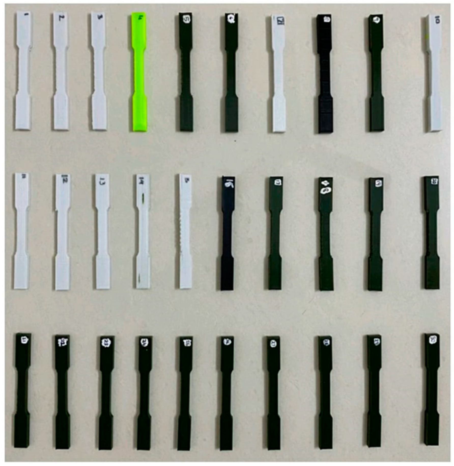
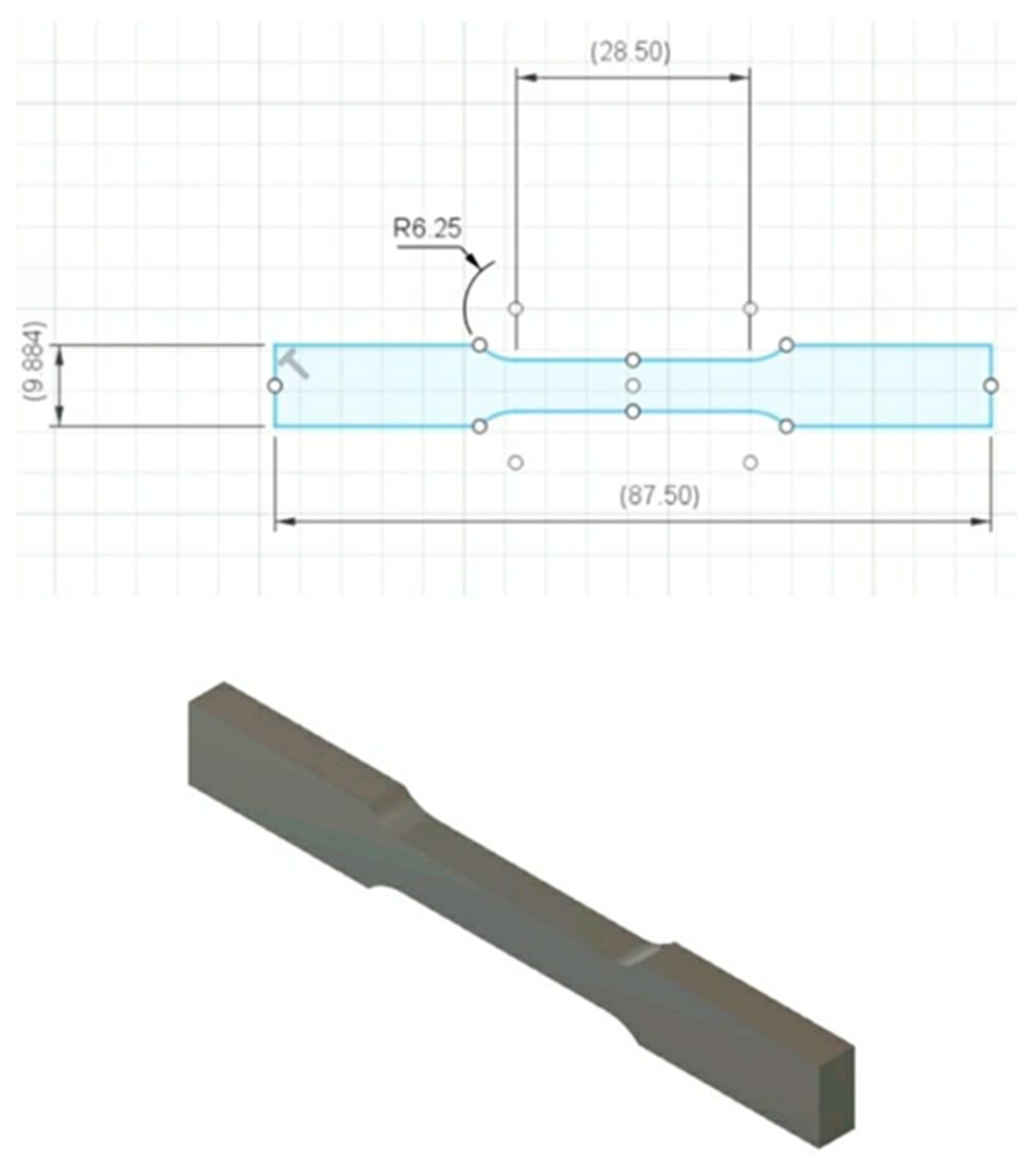
To ensure consistency in the model, the ASTM E8 standard geometry was adopted as the reference with a uniform 50% reduction in dimensions to reduce print size, minimize material usage and time. The Response Surface Methodology (RSM) Design of Experiment was employed to generate 30 different trial conditions (refer to
Figure 1), each with three input parameter levels. The CAD model (refer to
Figure 2) was sliced using Ultimaker Cura software to generate G-code. The Creality 3D FDM printer (refer to
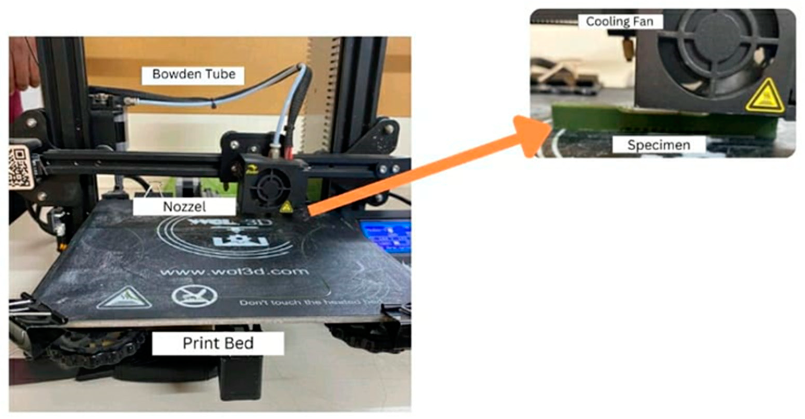
Figure 3) was used to carry out the experimental investigation. Each print was assigned a unique set of settings varying in layer height, infill density, infill pattern, bed temperature, and nozzle temperature to fabricate Polyactic Acid (PLA) specimens. An input parameter datasheet was created, and the differences in length between each model and the original CAD file were measured using a digital vernier caliper.
The obtained experimental data is converted into a CSV file and is further imported to a Google Colab platform for deploying Supervised Machine Learning regression-based algorithms developed using Python programming.
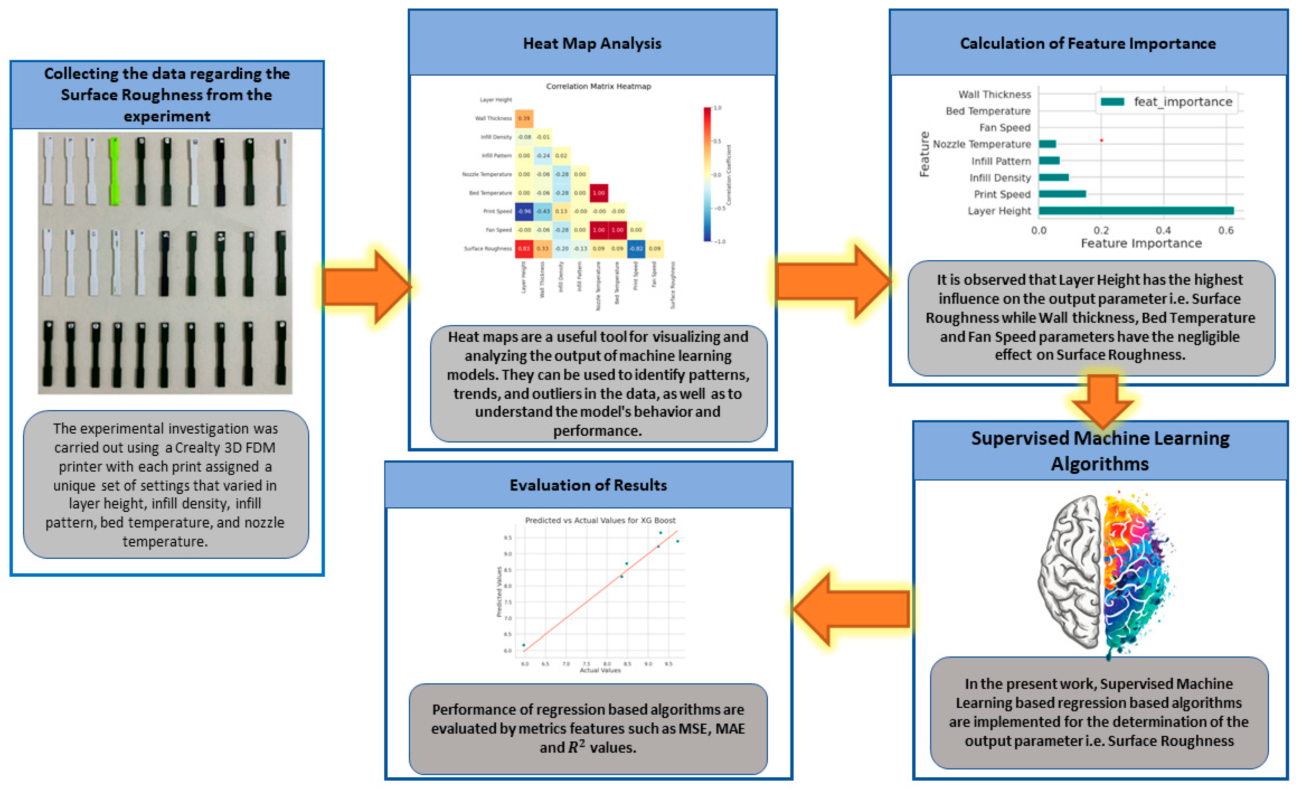
Figure 4 shows the implemented framework in the present work. Pandas library used for data manipulation and analysis. It provides data structures for efficiently storing and accessing large datasets. Pandas is widely used in machine learning for tasks such as data preprocessing, cleaning, and transformation. It allows for the handling of missing values, merging and grouping of datasets, and filtering and sorting of data. NumPy is used extensively in machine learning. It provides support for large multi-dimensional arrays and matrices, along with a collection of high-level mathematical functions. NumPy is useful in machine learning for tasks such as linear algebra, numerical computing, and scientific computing. Seaborn library is used for data visualization. It provides a high-level interface for creating attractive and informative statistical graphics. Seaborn is useful in machine learning for visualizing data distributions, detecting patterns, and exploring relationships between variables. Matplotlib is another Python library used for data visualization. It is a comprehensive library that provides a wide range of graphical tools for creating high-quality visualizations. Matplotlib is useful in machine learning for tasks such as data visualization, model evaluation, and result presentation.
In machine learning, a critical aspect of building a model is evaluating its performance. To do this, data scientists divide the dataset into two parts: training data and testing data. Typically, 80% of the dataset is used for training, while the remaining 20% is used for testing. The primary reason for using the 80/20 split is to reduce overfitting, which occurs when a model is too complex and fits the training data too closely. By using a smaller portion of the dataset for testing, data scientists can ensure that the model generalizes well to new data.
In the present work, Mean Absolute Error (MAE), Mean Square Error (MSE) and coefficient of determination (R2) are the metric features used for measuring the performance of machine learning models. MAE is a popular metric feature for evaluating the performance of regression models. It is the average of the absolute differences between the predicted values and the actual values. The lower the value of MAE, the better the performance of the model. MAE is used because it provides an easily interpretable measure of the average magnitude of the errors in the predicted values. MSE is another popular metric feature for evaluating the performance of regression models. It is the average of the squared differences between the predicted values and the actual values. MSE is used because it penalizes large errors more heavily than small ones, which is important in accurately evaluating the model's performance. R2 is a statistical measure that represents the proportion of the variance in the dependent variable that is explained by the independent variables in the model. R-squared values range from 0 to 1, with higher values indicating a better fit of the model to the data. R-squared is a useful metric feature for evaluating regression models because it provides insight into the model's ability to explain the variation in the data.
3. Results
Table 1 shows the obtained results for Surface roughness by the combination of different input parameters.
3.1. Supervised Machine Learning Algorithms
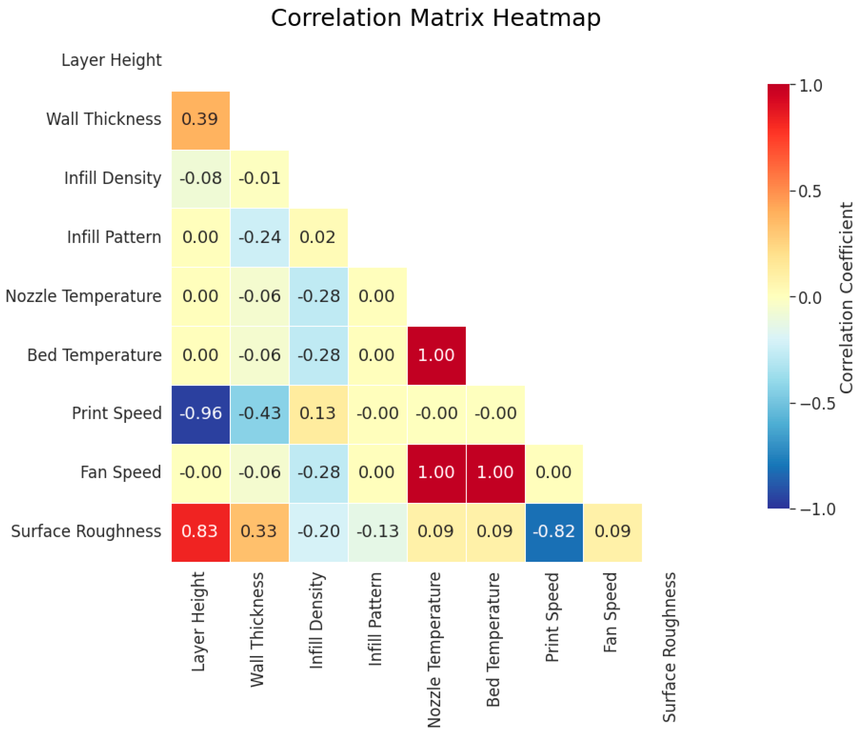
Figure 5 shows the obtained Confusion Heat Map matrix in the present work. Correlation matrix heatmap is an essential tool in machine learning because it helps to identify the strength and direction of the relationship between different variables. It provides a quick visual representation of how different variables are related to each other. This information is critical in feature selection, as highly correlated variables can lead to overfitting, and it is important to remove redundant variables to improve the model's performance. The correlation matrix heatmap is color-coded, with the intensity of the color representing the strength of the correlation. A positive correlation is represented by a shade of blue, while a negative correlation is represented by a shade of red. The darker the shade, the stronger the correlation. A neutral correlation is represented by a shade of white or gray. Variables that are highly correlated with each other appear as dark squares on the heatmap. These variables can lead to overfitting and should be removed. Variables that have little or no correlation with each other appear as light squares on the heatmap. Negative correlation between two variables is represented by a shade of red. If the variables have a strong negative correlation, it means that they move in opposite directions. Positive correlation between two variables is represented by a shade of blue. If the variables have a strong positive correlation, it means that they move in the same direction.
Figure 6 shows the feature importance plot obtained in the present work. Feature importance plot is a visual tool used in machine learning to determine the importance of each feature in a dataset. It helps in identifying which features are most relevant to the target variable and which can be eliminated. The feature importance plot can also help in identifying irrelevant features that do not contribute to the model's accuracy. These features can be eliminated during feature selection to improve the model's performance. It is observed that Layer Height has the highest influence on the output parameter i.e. Surface Roughness while Wall thickness, Bed Temperature and Fan Speed parameters have the negligible effect on Surface Roughness.
Table 2 shows the comparison of the performance of implemented supervised machine learning regression based algorithms on the basis of metric features such as MSE, MAE and R2 value.
Figure 7 shows the obtained decision tree plot. Decision tree plots are crucial in machine learning as they provide a visual representation of the decision-making process used by a model. These plots show the hierarchy of decision rules used to classify or predict outcomes and help in interpreting the model's behavior. The information obtained from a decision tree plot can help in understanding the important features that contribute to the model's accuracy and identify areas where the model can be improved. Additionally, decision tree plots can aid in explaining the model's predictions to non-technical stakeholders, making it an essential tool for both model developers and end-users. Therefore, decision tree plots are an important component of the machine learning toolkit and can provide valuable insights into the underlying decision-making process of a model.
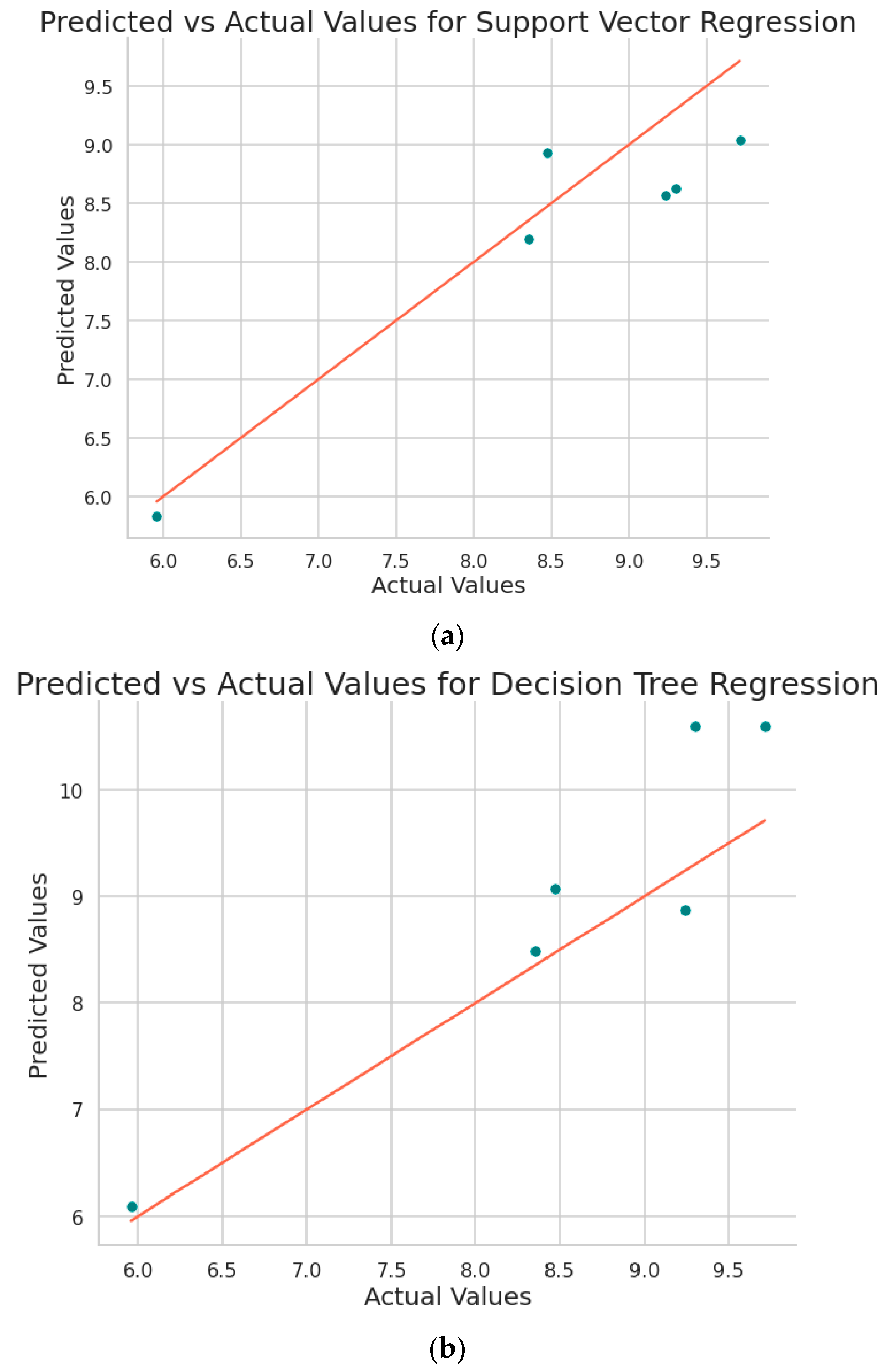
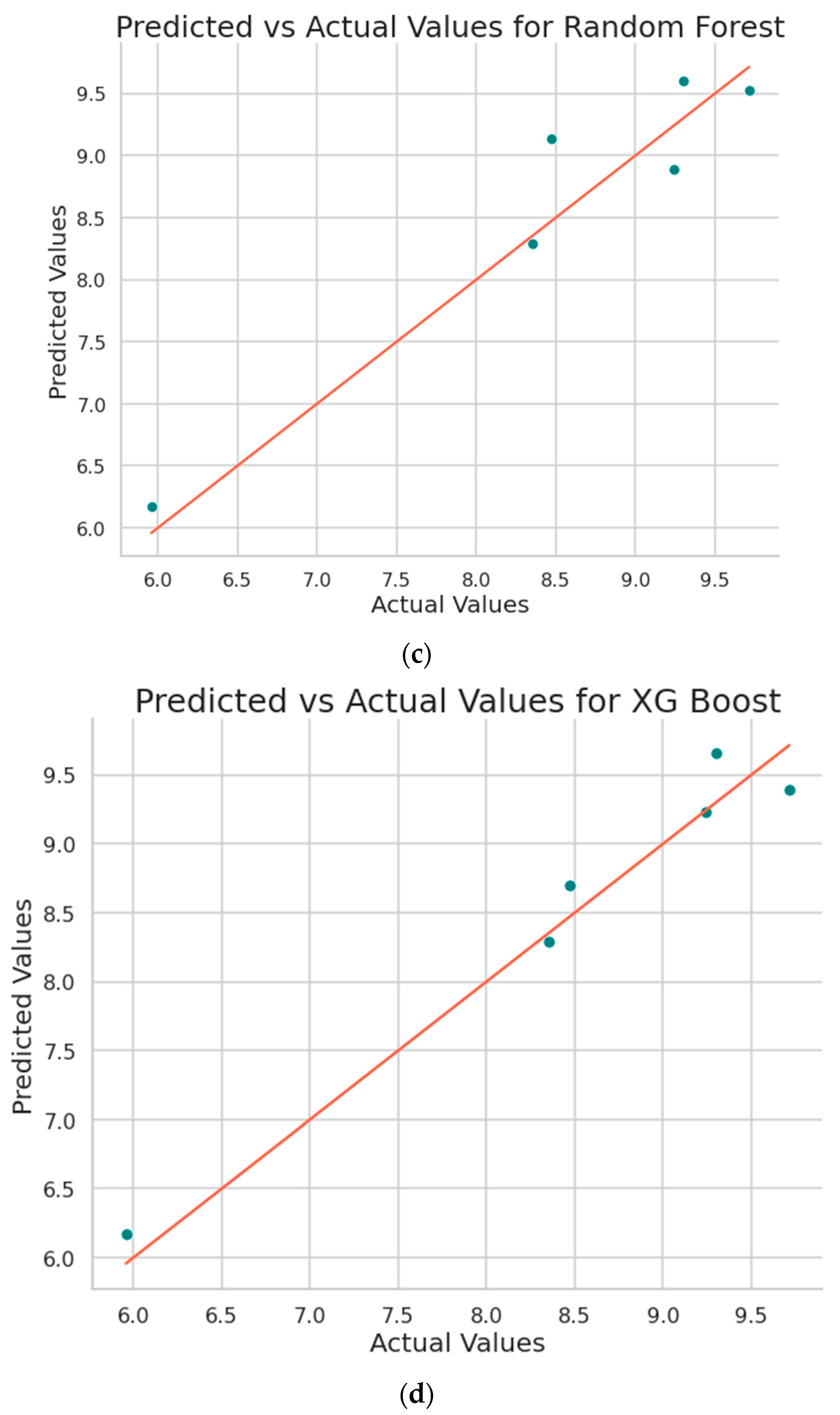
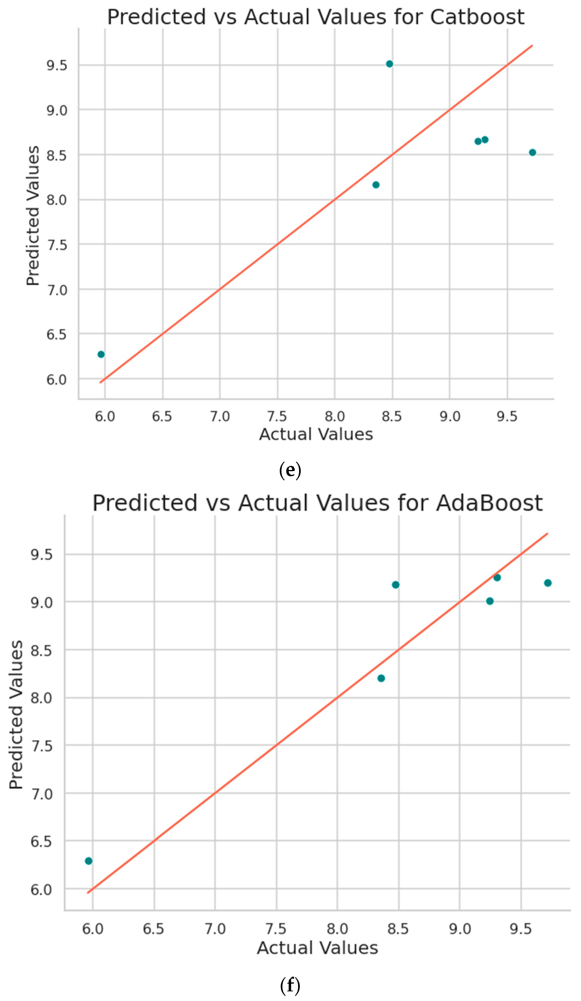
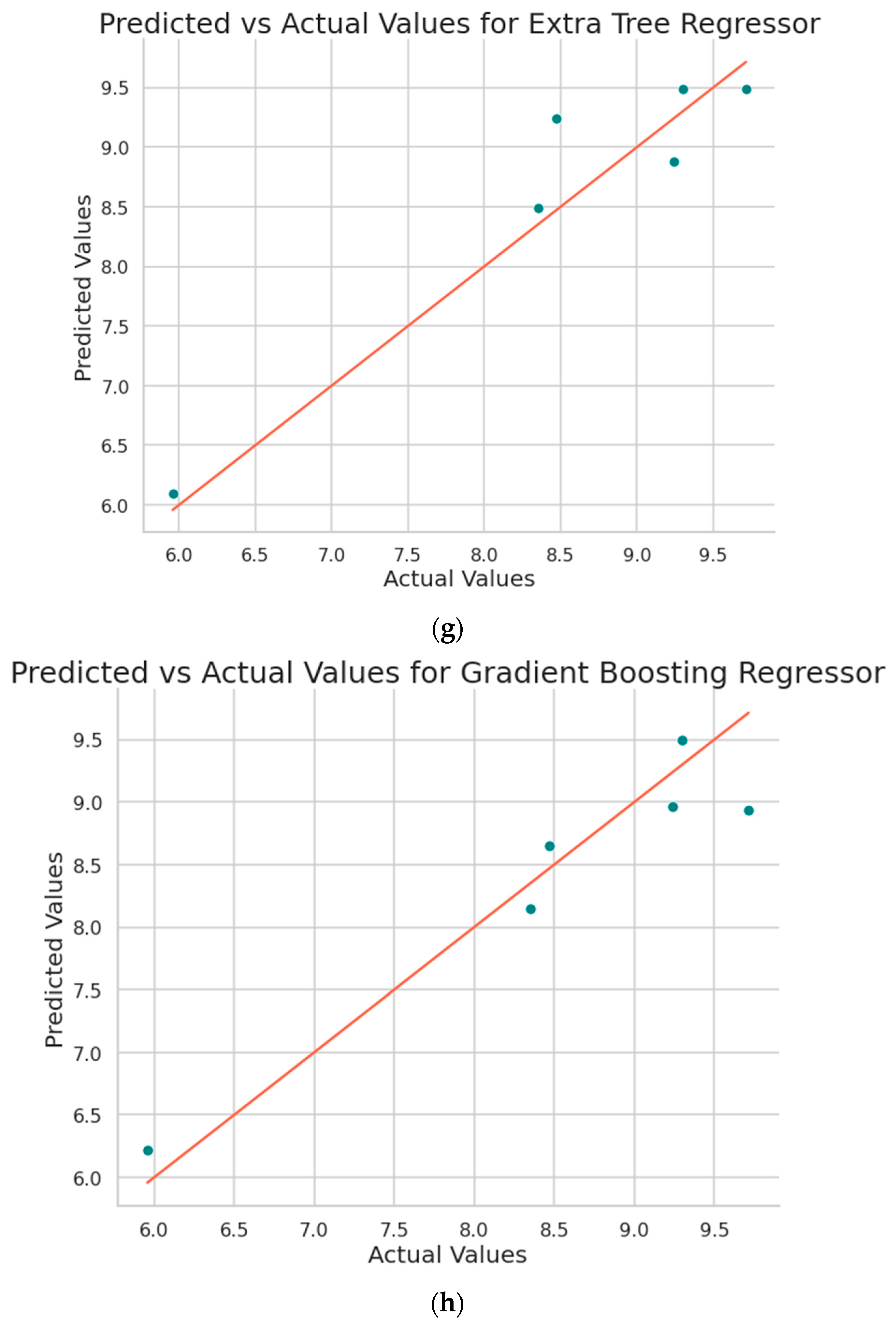
Figure 8 shows the plot obtained between the predicted values and the original values from the implemented machine learning algorithms.
3.2. Explainable Artificial Intelligence (XAI) Approach
Explainable AI (XAI) aims to provide human-understandable explanations for the decisions made by machine learning models. In your case, you have a set of input parameters that influence the surface roughness of additive manufactured specimens. XAI can be applied to make the relationship between these input parameters and surface roughness more transparent and interpretable.
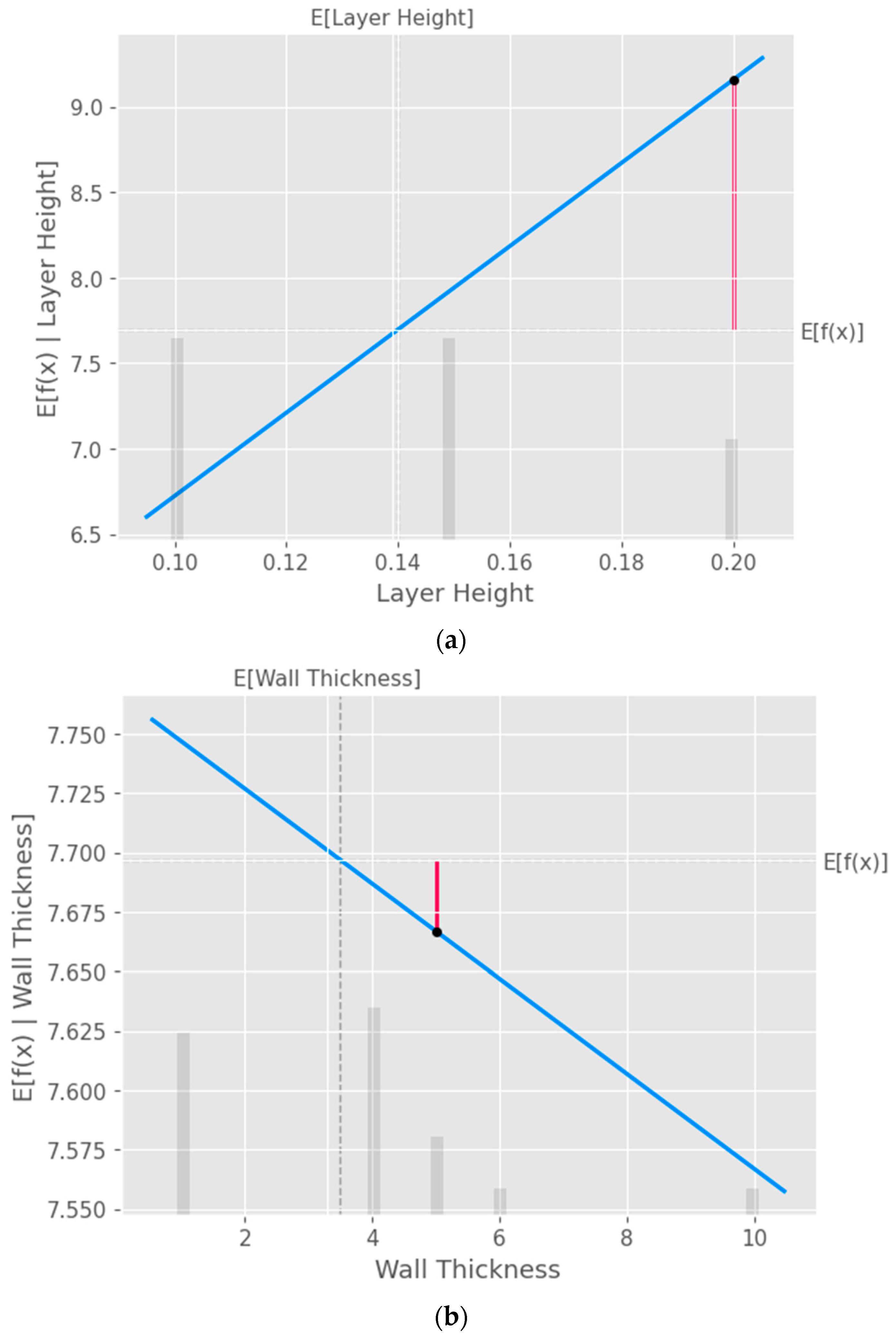
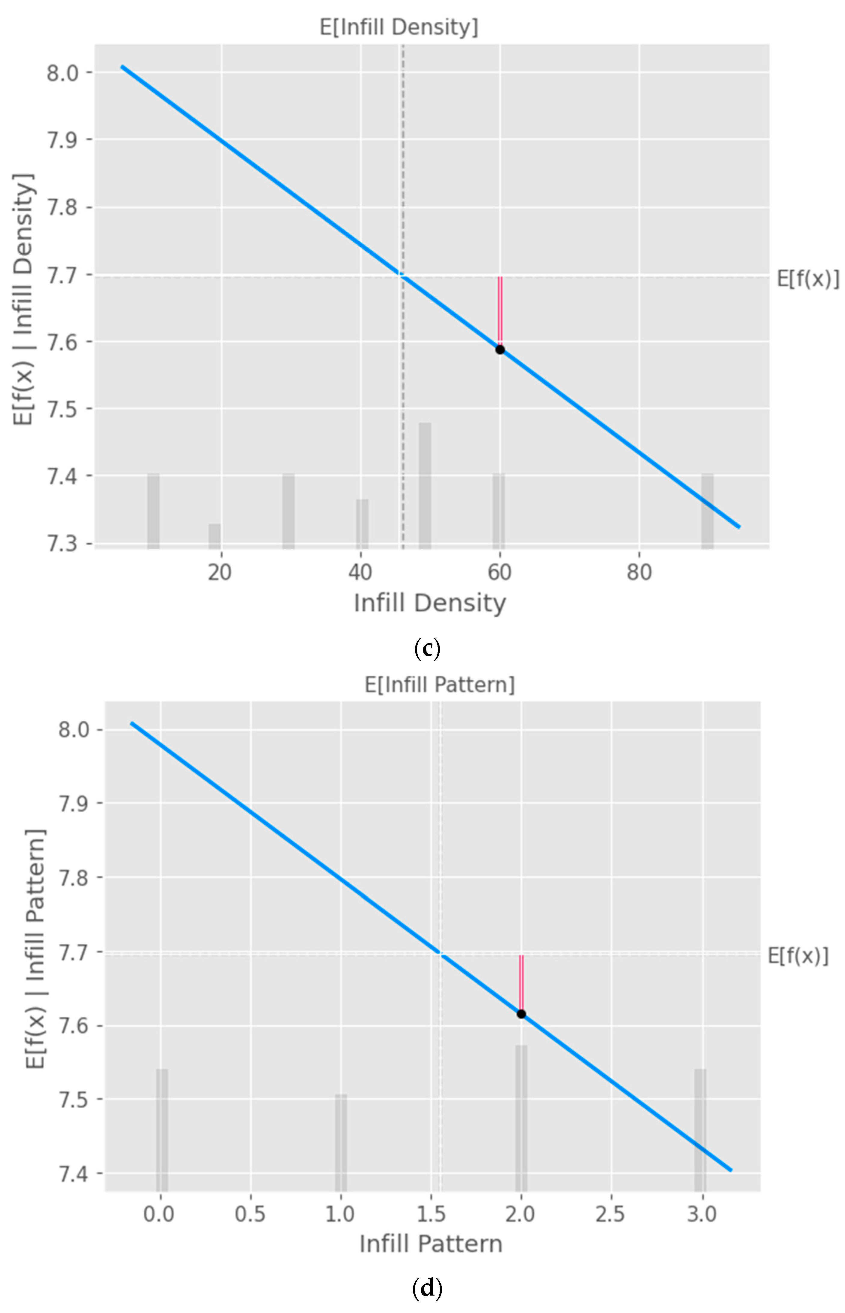
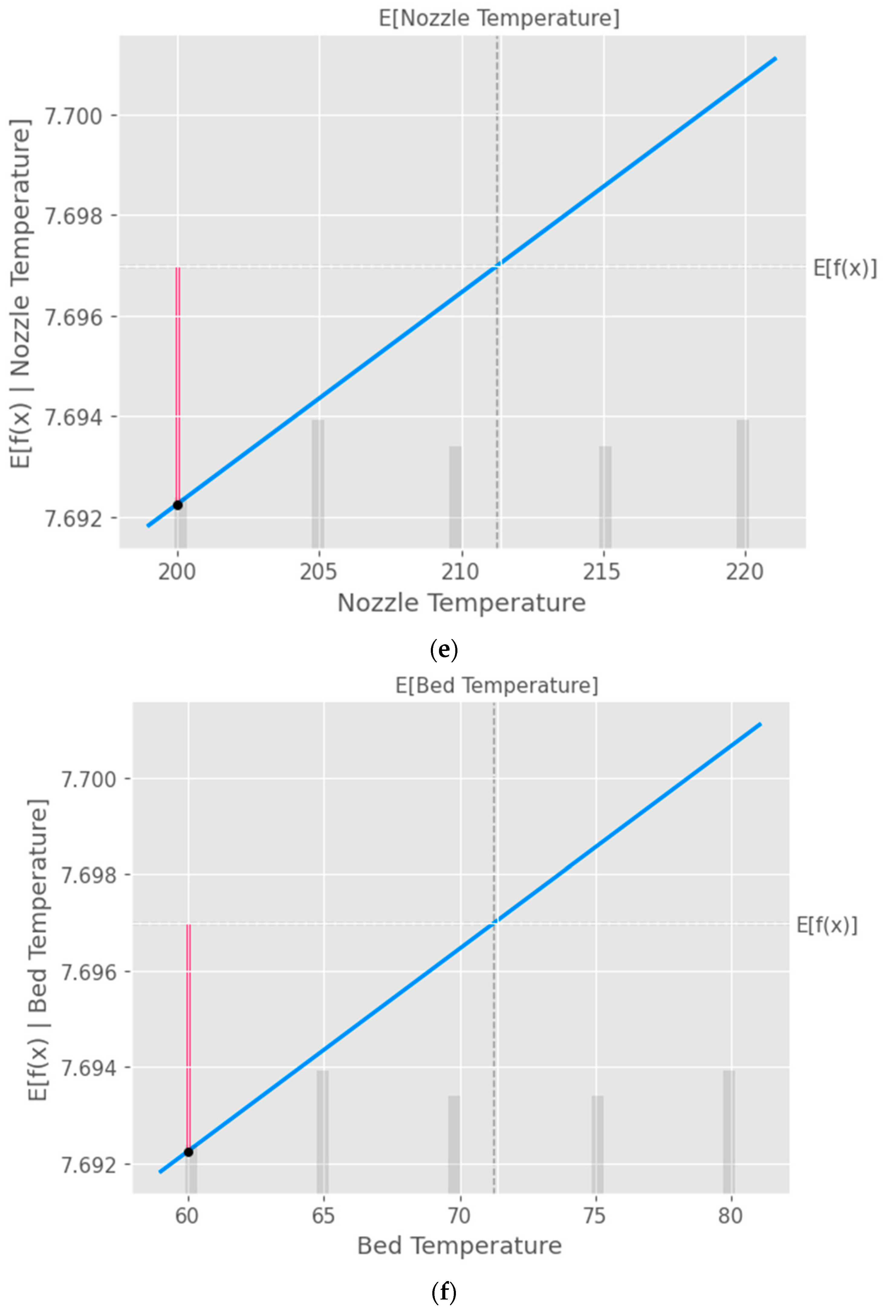
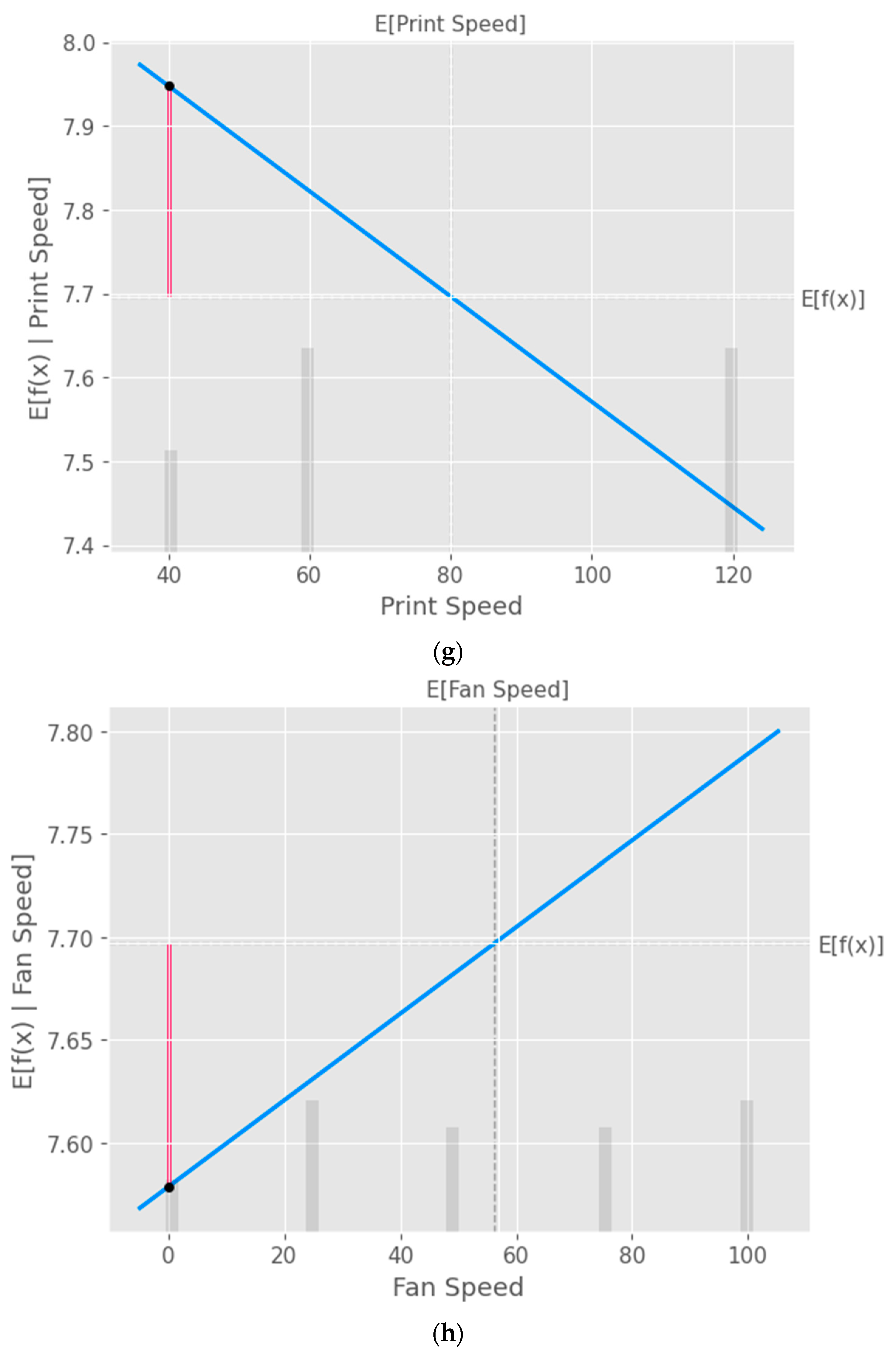
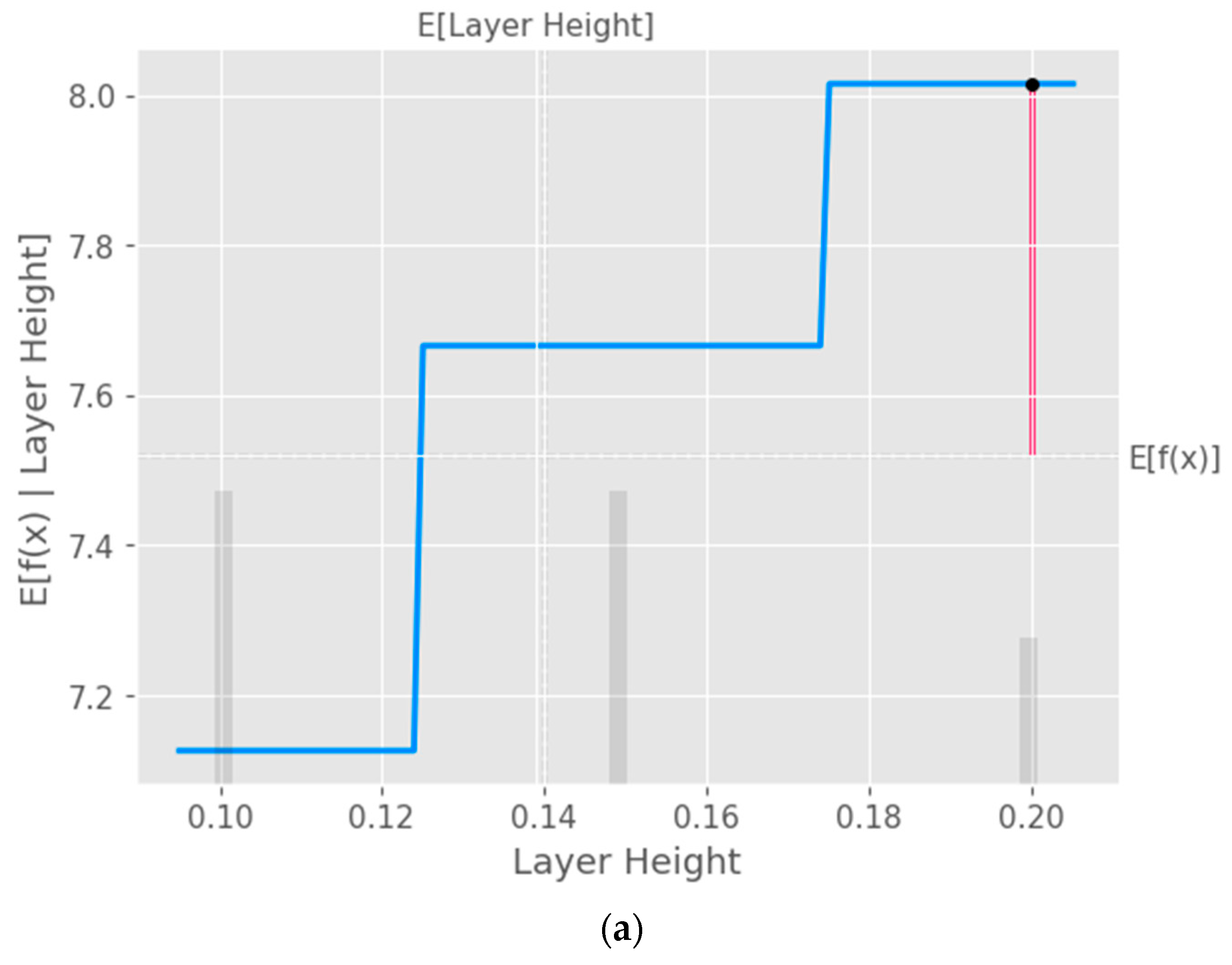
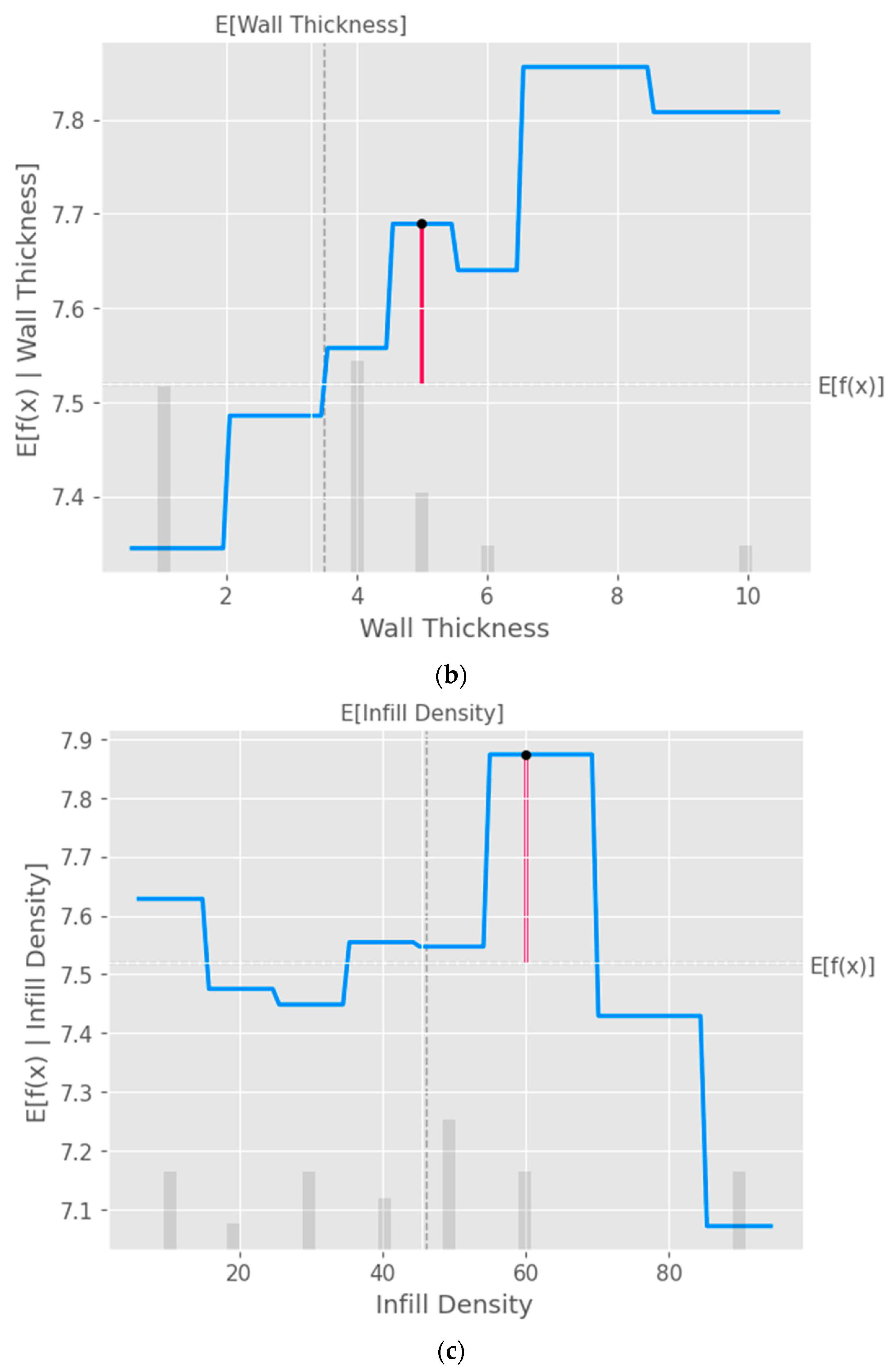
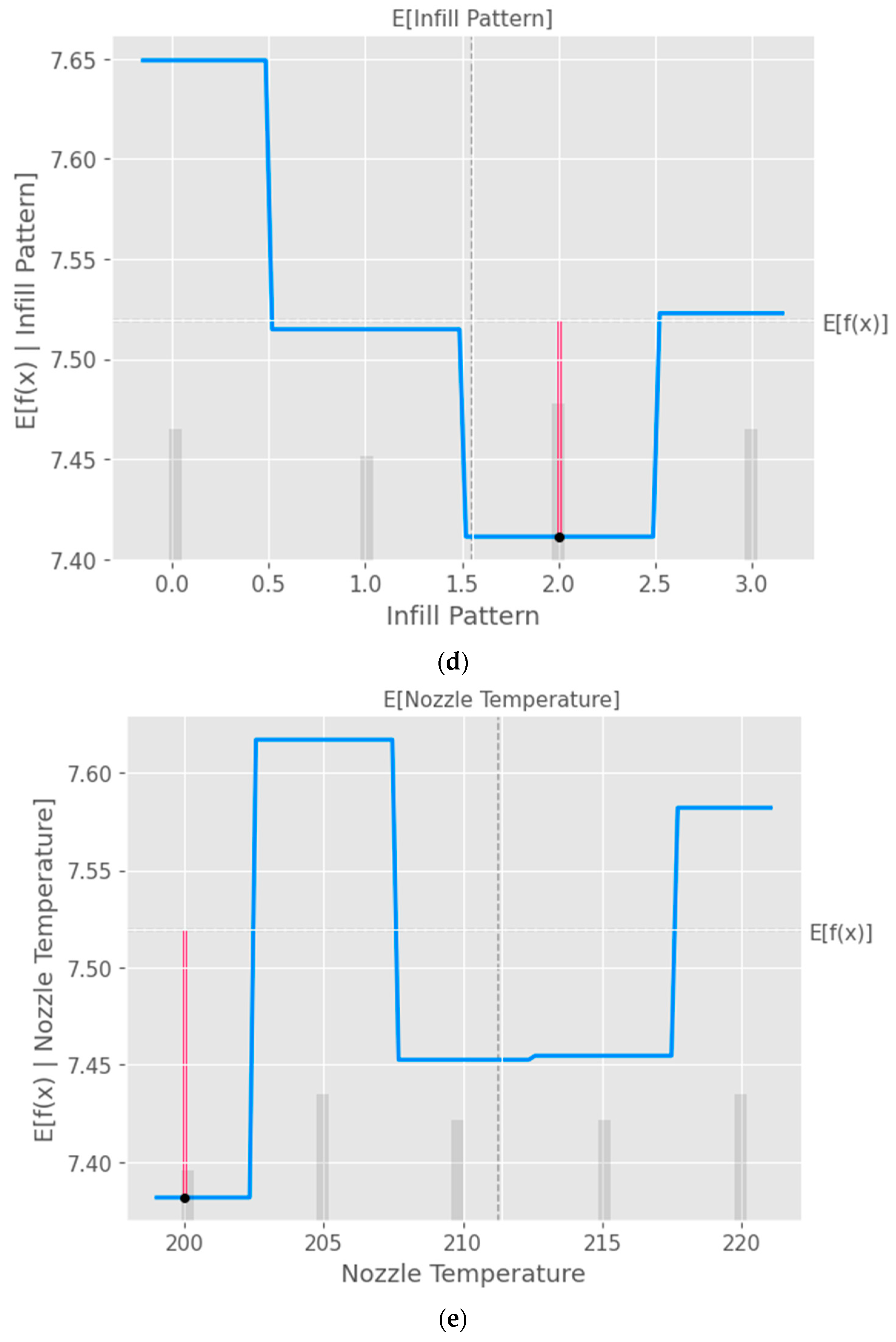
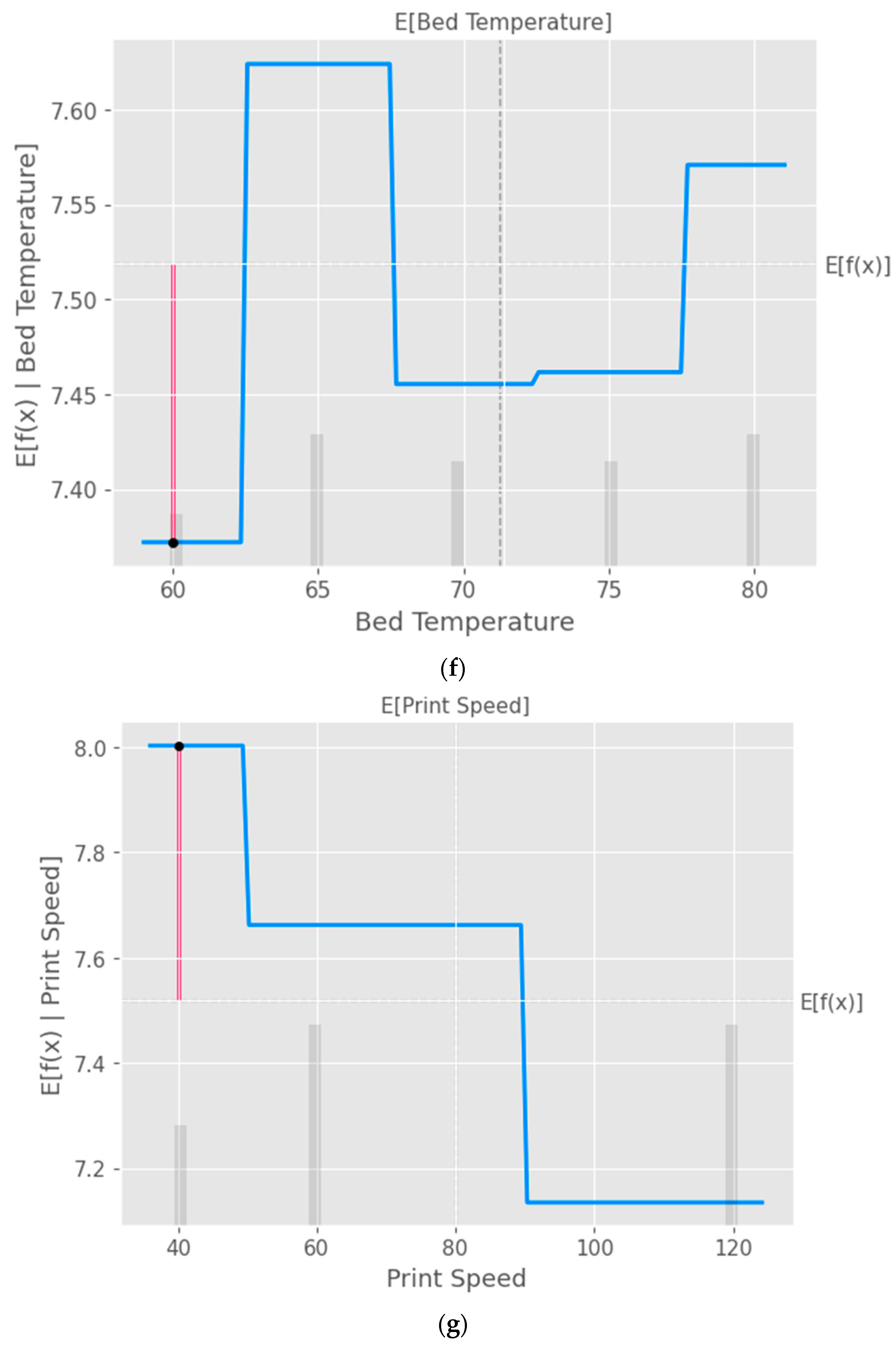
The partial dependence plot created using SHAP values as shown in
Figure 9 provides valuable insights into the relationship between a specific input feature and the model's predictions. This plot can be used to analyze the effect of the chosen feature on the predicted output while accounting for the average influence of all other features. By interpreting this plot, researchers can gain a deeper understanding of the model's behavior and make informed decisions.
A waterfall plot shown in
Figure 10 is a visual representation that helps to understand the step-by-step contributions of individual features to a model's prediction for a specific instance. This plot is useful for interpreting the model's behavior and attributing importance to each feature in a clear, ordered manner.
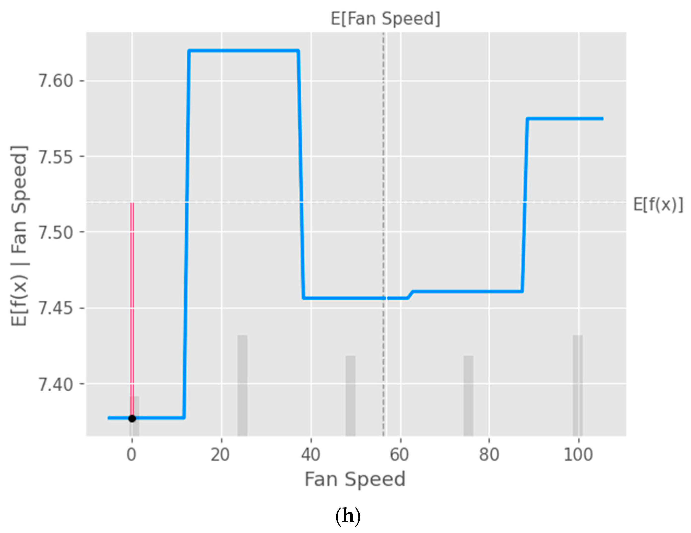
Figure 11 demonstrates the process of fitting an Explainable Boosting Machine (EBM) model to the data and using SHAP values to create a partial dependence plot for the input features. EBM is a type of Generalized Additive Model (GAM) that provides interpretable results through additive combinations of simple models.
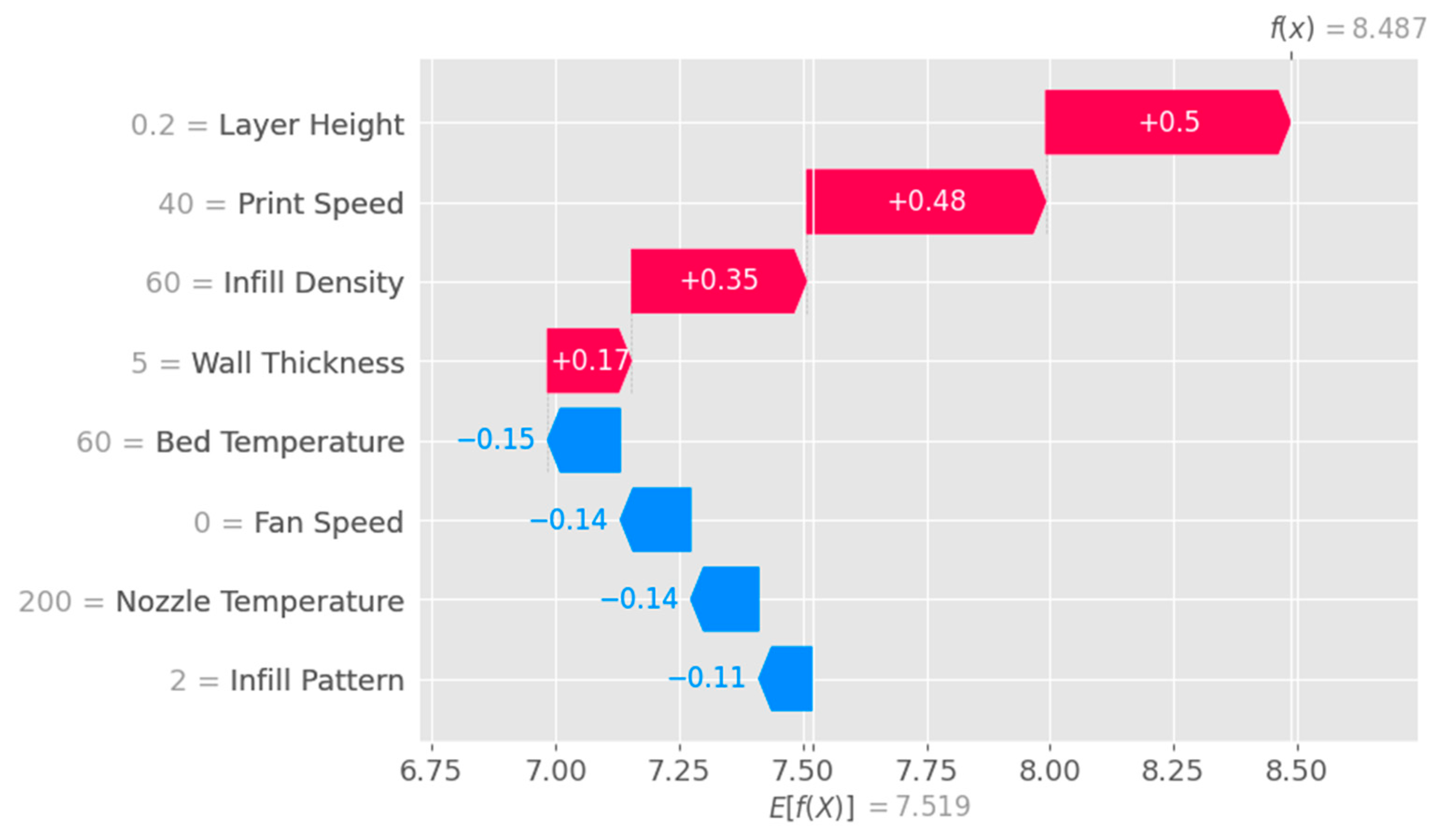
Figure 12 shows a waterfall plot using SHAP values obtained from the Explainable Boosting Machine (EBM) model.
The main difference between the two waterfall plots lies in the model they are based on. The first waterfall plot is created using the SHAP values obtained from the linear model, while the second waterfall plot is created using the SHAP values obtained from the Explainable Boosting Machine (EBM) model.
The linear model and the EBM model are distinct in their underlying assumptions, complexity, and interpretability. The EBM model is a type of Generalized Additive Model (GAM) that provides more interpretable results by combining simple models additively, while a linear model is based on a linear combination of input features. These differences in the model structures can lead to different feature contributions and importance rankings in the two waterfall plots.
The interpretation of both waterfall plots is similar, as they both provide insights into the step-by-step contributions of individual features to a model's prediction for a specific instance. However, the actual contributions of features and their importance rankings may differ between the two plots due to the differences in the underlying models. Comparing the two waterfall plots can help identify any discrepancies or similarities in feature contributions between the linear model and the EBM model, potentially leading to a better understanding of the relationships between the input features and the target variable.
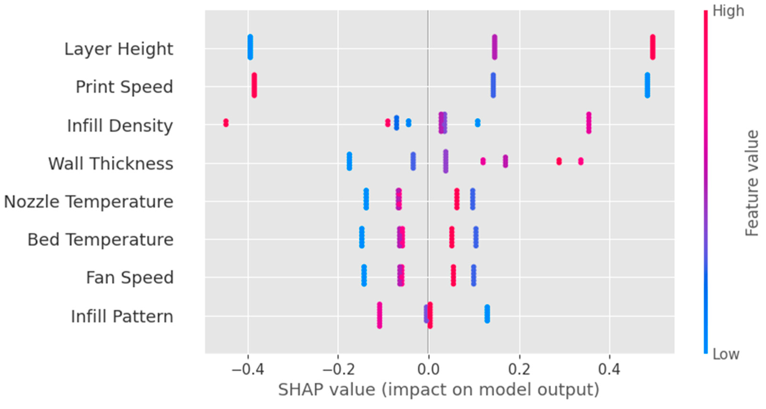
The Bee swarm plot as shown in
Figure 13 is a powerful visualization tool that displays the SHAP values for all features and instances in the dataset. It helps to understand the overall impact of each feature on the model's predictions and offers insights into the distribution of feature contributions across all instances.
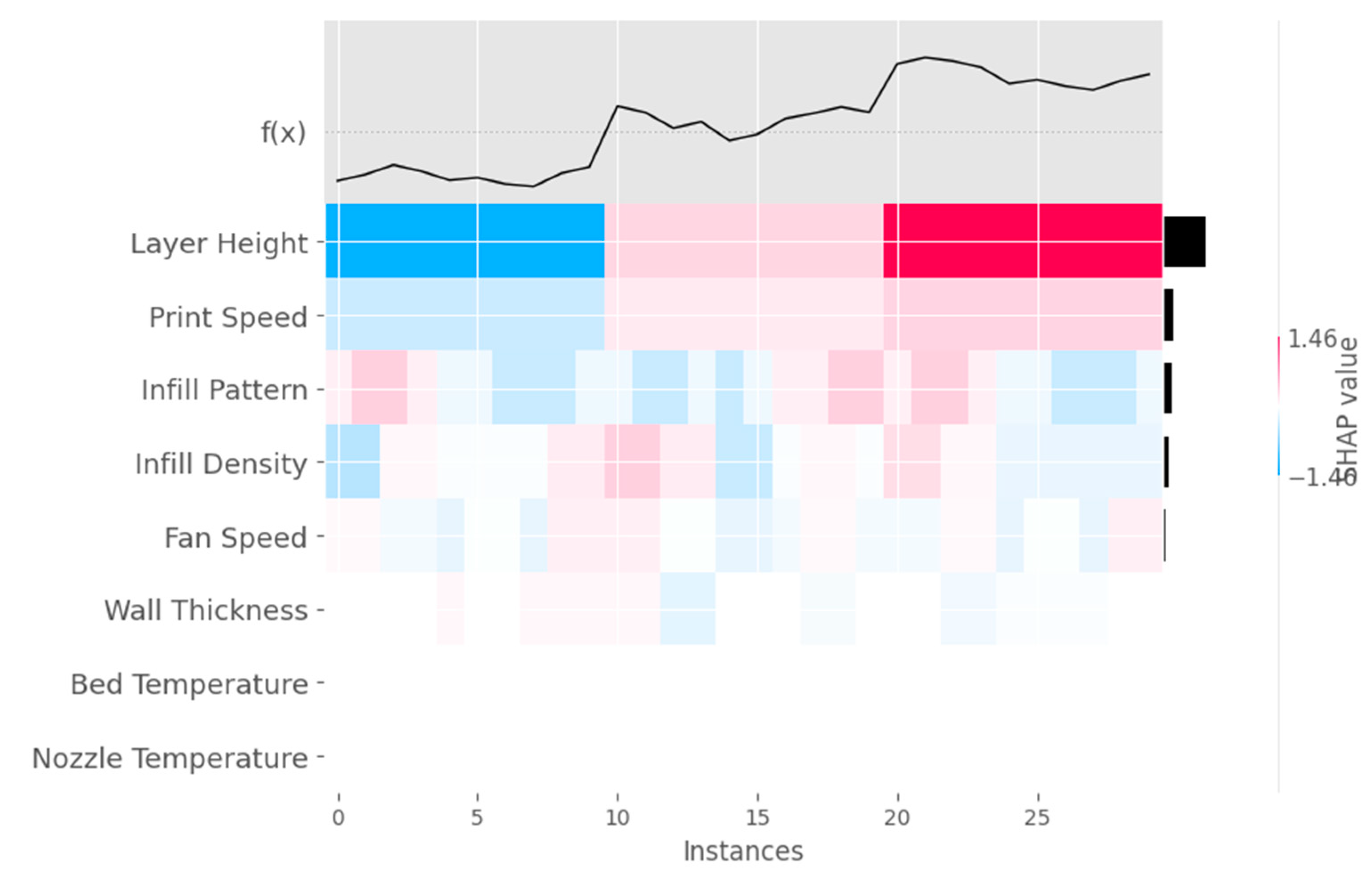
The Heat map plot as shown in
Figure 14 is a visualization tool that displays SHAP values for all features and a subset of instances in the dataset as a heatmap. It helps to understand the impact of each feature on the model's predictions and offers insights into the distribution of feature contributions across the selected instances.
4. Discussion
From the obtained results it is observed that XG Boost algorithm outperforms other machine learning algorithms by resulting in highest R2 value. XGBoost is a highly effective machine learning algorithm due to its scalability, regularization techniques, speed, handling of missing data, feature importance, and flexibility. It is optimized for parallel processing on multi-core CPUs, allowing it to handle large datasets with millions of examples and features efficiently. XGBoost uses both L1 and L2 regularization techniques to prevent overfitting and improve the model's generalization performance, and it can handle missing data effectively using gradient-based sampling. XGBoost provides a measure of feature importance, allowing for the identification of significant features in the dataset, and it is flexible, handling both regression and classification tasks. These features make XGBoost a popular choice for many machine learning tasks, and it is often used as a benchmark for other algorithms.
Explainable AI (XAI) is of paramount importance in the present research work for several reasons. In the context of predicting surface roughness for additive manufactured specimens, employing XAI techniques can enhance the understanding, trust, and effectiveness of the developed models, which in turn can lead to better decision-making and improved outcomes. individual features to the model's predictions. This interpretability enables researchers to gain insights into the relationships between input features and the target variable (surface roughness), leading to a better understanding of the underlying physical processes involved in additive manufacturing. By providing clear explanations of how the model makes predictions, XAI enhances the trust that stakeholders have in the model. This is crucial in engineering applications, such as additive manufacturing, where the quality and performance of produced components are vital. Trustworthy models can facilitate the adoption of AI-driven solutions in industry and help ensure that the developed models are used effectively.XAI techniques can aid in validating the developed models by revealing the contributions of each feature and detecting any biases or inconsistencies. By examining the feature importances and potential interaction effects, researchers can evaluate the models and identify any areas that require further improvement, ultimately leading to more accurate and reliable predictions. XAI enables researchers to communicate their findings more effectively, both within the research community and to industry stakeholders. Clear, interpretable visualizations, such as partial dependence plots, beeswarm plots, and heatmap plots, can convey complex relationships and model behavior in an accessible manner. This facilitates better collaboration and understanding among researchers, engineers, and decision-makers involved in the additive manufacturing process. In some industries, including additive manufacturing, regulatory compliance may require explanations for AI-driven decisions. XAI techniques can provide the necessary transparency and interpretability to meet these regulatory requirements, ensuring that AI solutions can be successfully implemented in real-world applications.
5. Conclusions
In conclusion, this research work presents a comprehensive analysis of the prediction of surface roughness in additive manufactured Polyactic Acid (PLA) specimens using eight different supervised machine learning regression-based algorithms. The results demonstrate the superiority of the XG Boost algorithm, with the highest coefficient of determination value of 0.9634, indicating its ability to accurately predict surface roughness. Additionally, this study pioneers the use of Explainable AI techniques to enhance the interpretability of machine learning models, offering valuable insights into feature importance, interaction effects, and model behavior. The comparative analysis of the algorithms, combined with the explanations provided by Explainable AI, contributes to a better understanding of the relationship between surface roughness and structural integrity in additive manufacturing.
Author Contributions
Conceptualization, A.M., V.S.J, E.M.S and S.P.; methodology, A.M.; software, V.S.J.; validation, S.P., E.M.S and A.M.; formal analysis, S.P.; investigation, V.S.J.; resources, S.P.; data curation, V.S.J.; writing—original draft preparation, A.M.; writing—review and editing, E.M.S.; visualization, S.P.; supervision, V.S.J.; project administration, V.S.J. All authors have read and agreed to the published version of the manuscript.
Data Availability Statement
Data will be available upon request by the readers.
Conflicts of Interest
The authors declare no conflict of interest.
References
- Badillo, S.; Banfai, B.; Birzele, F.; Davydov, I.I.; Hutchinson, L.; Kam-Thong, T.; Siebourg-Polster, J.; Steiert, B.; Zhang, J.D. An introduction to machine learning. Clin. Pharmacol. Ther. 2020, 107, 871–885. [Google Scholar] [CrossRef] [PubMed]
- Kubat, M.; Kubat, J.A. An Introduction to Machine Learning; Springer International Publishing: Cham, Switzerland, 2017; Volume 2, pp. 321–329. [Google Scholar]
- Choi, R.Y.; Coyner, A.S.; Kalpathy-Cramer, J.; Chiang, M.F.; Campbell, J.P. Introduction to machine learning, neural networks, and deep learning. Transl. Vis. Sci. Technol. 2020, 9, 14. [Google Scholar] [PubMed]
- El Bouchefry, K.; de Souza, R.S. Learning in big data: Introduction to machine learning. In Knowledge Discovery in Big Data from Astronomy and Earth Observation; Elsevier: Amsterdam, The Netherlands, 2020; pp. 225–249. [Google Scholar]
- Burkart, N.; Huber, M.F. A survey on the explainability of supervised machine learning. J. Artif. Intell. Res. 2021, 70, 245–317. [Google Scholar] [CrossRef]
- Jiang, T.; Gradus, J.L.; Rosellini, A.J. Supervised machine learning: A brief primer. Behav. Ther. 2020, 51, 675–687. [Google Scholar] [CrossRef] [PubMed]
- Fukami, K.; Fukagata, K.; Taira, K. Assessment of supervised machine learning methods for fluid flows. Theor. Comput. Fluid Dyn. 2020, 34, 497–519. [Google Scholar] [CrossRef]
- Alloghani, M.; Al-Jumeily, D.; Mustafina, J.; Hussain, A.; Aljaaf, A.J. A systematic review on supervised and unsupervised machine learning algorithms for data science. In Supervised and Unsupervised Learning for Data Science; Springer: Berlin/Heidelberg, Germany, 2020; pp. 3–21. [Google Scholar]
- Kim, B.; Yuvaraj, N.; Tse, K.T.; Lee, D.E.; Hu, G. Pressure pattern recognition in buildings using an unsupervised machine-learning algorithm. J. Wind. Eng. Ind. Aerodyn. 2021, 214, 104629. [Google Scholar] [CrossRef]
- Kadiyala, P.; Shanmukhasai, K.V.; Budem, S.S.; Maddikunta, P.K.R. Anomaly Detection Using Unsupervised Machine Learning Algorithms. In Deep Learning for Security and Privacy Preservation in IoT; Springer Singapore: Singapore, 2022; pp. 113–125. [Google Scholar]
- Botvinick, M.; Ritter, S.; Wang, J.X.; Kurth-Nelson, Z.; Blundell, C.; Hassabis, D. Reinforcement learning, fast and slow. Trends Cogn. Sci. 2019, 23, 408–422. [Google Scholar] [CrossRef] [PubMed]
- Laskin, M.; Lee, K.; Stooke, A.; Pinto, L.; Abbeel, P.; Srinivas, A. Reinforcement learning with augmented data. Adv. Neural Inf. Process. Syst. 2020, 33, 19884–19895. [Google Scholar]
- Yarats, D.; Fergus, R.; Lazaric, A.; Pinto, L. Reinforcement learning with prototypical representations. In Proceedings of the International Conference on Machine Learning, Virtual, 1 July 2021; pp. 11920–11931. [Google Scholar]
- Blakey-Milner, B.; Gradl, P.; Snedden, G.; Brooks, M.; Pitot, J.; Lopez, E.; Leary, M.; Berto, F.; du Plessis, A. Metal additive manufacturing in aerospace: A review. Mater. Des. 2021, 209, 110008. [Google Scholar] [CrossRef]
- Zhu, J.; Zhou, H.; Wang, C.; Zhou, L.; Yuan, S.; Zhang, W. A review of topology optimization for additive manufacturing: Status and challenges. Chin. J. Aeronaut. 2021, 34, 91–110. [Google Scholar] [CrossRef]
- Abdulhameed, O.; Al-Ahmari, A.; Ameen, W.; Mian, S.H. Additive manufacturing: Challenges, trends, and applications. Adv. Mech. Eng. 2019, 11, 1687814018822880. [Google Scholar] [CrossRef]
- Liu, G.; Zhang, X.; Chen, X.; He, Y.; Cheng, L.; Huo, M.; Yin, J.; Hao, F.; Chen, S.; Wang, P.; et al. Additive manufacturing of structural materials. Mater. Sci. Eng. R Rep. 2021, 145, 100596. [Google Scholar] [CrossRef]
- Wang, C.; Tan, X.P.; Tor, S.B.; Lim, C.S. Machine learning in additive manufacturing: State-of-the-art and perspectives. Addit. Manuf. 2020, 36, 101538. [Google Scholar] [CrossRef]
- Qin, J.; Hu, F.; Liu, Y.; Witherell, P.; Wang, C.C.; Rosen, D.W.; Simpson, T.; Lu, Y.; Tang, Q. Research and application of machine learning for additive manufacturing. Addit. Manuf. 2022, 52, 102691. [Google Scholar] [CrossRef]
- Qi, X.; Chen, G.; Li, Y.; Cheng, X.; Li, C. Applying neural-network-based machine learning to additive manufacturing: Current applications, challenges, and future perspectives. Engineering 2019, 5, 721–729. [Google Scholar] [CrossRef]
- Gockel, J.; Sheridan, L.; Koerper, B.; Whip, B. The influence of additive manufacturing processing parameters on surface roughness and fatigue life. Int. J. Fatigue 2019, 124, 380–388. [Google Scholar] [CrossRef]
- Maleki, E.; Bagherifard, S.; Bandini, M.; Guagliano, M. Surface post-treatments for metal additive manufacturing: Progress, challenges, and opportunities. Addit. Manuf. 2021, 37, 101619. [Google Scholar] [CrossRef]
- Whip, B.; Sheridan, L.; Gockel, J. The effect of primary processing parameters on surface roughness in laser powder bed additive manufacturing. Int. J. Adv. Manuf. Technol. 2019, 103, 4411–4422. [Google Scholar] [CrossRef]
- Nakatani, M.; Masuo, H.; Tanaka, Y.; Murakami, Y. Effect of surface roughness on fatigue strength of Ti-6Al-4V alloy manufactured by additive manufacturing. Procedia Struct. Integr. 2019, 19, 294–301. [Google Scholar] [CrossRef]
Figure 1.
30 specimens fabricated in the present work.
Figure 1.
30 specimens fabricated in the present work.
Figure 2.
Design of the additively manufactured specimen.
Figure 2.
Design of the additively manufactured specimen.
Figure 3.
Setup for 3D printing the specimens.
Figure 3.
Setup for 3D printing the specimens.
Figure 4.
Implemented machine learning framework in the present work.
Figure 4.
Implemented machine learning framework in the present work.
Figure 5.
Correlation Matrix heatmap plot.
Figure 5.
Correlation Matrix heatmap plot.
Figure 6.
Feature Importance plot.
Figure 6.
Feature Importance plot.
Figure 7.
Decision Tree Plot.
Figure 7.
Decision Tree Plot.
Figure 8.
Predicted vs Actual surface roughness values plot obtained by a) Support Vector Regression b) Decision Tree c) Random Forest d) XG Boost e) Cat Boost f) Ada Boost g) Extra Tree Regressor h) Gradient Boosting regressor.
Figure 8.
Predicted vs Actual surface roughness values plot obtained by a) Support Vector Regression b) Decision Tree c) Random Forest d) XG Boost e) Cat Boost f) Ada Boost g) Extra Tree Regressor h) Gradient Boosting regressor.
Figure 9.
Partial Dependence Plot (PDP) of the input parameters a) Layer Height, b) Wall Thickness, c) Infill Density, d) Infill Pattern, e) Nozzle Temperature, f) Bed Temperature, g) Print Speed and h) Fan Speed.
Figure 9.
Partial Dependence Plot (PDP) of the input parameters a) Layer Height, b) Wall Thickness, c) Infill Density, d) Infill Pattern, e) Nozzle Temperature, f) Bed Temperature, g) Print Speed and h) Fan Speed.
Figure 11.
Partial Dependence Plot (PDP) taking EBM in consideration of the input parameters a) Layer Height, b) Wall Thickness, c) Infill Density, d) Infill Pattern, e) Nozzle Temperature, f) Bed Temperature, g) Print Speed and h) Fan Speed.
Figure 11.
Partial Dependence Plot (PDP) taking EBM in consideration of the input parameters a) Layer Height, b) Wall Thickness, c) Infill Density, d) Infill Pattern, e) Nozzle Temperature, f) Bed Temperature, g) Print Speed and h) Fan Speed.
Figure 12.
Waterfall plot with EBM Model.
Figure 12.
Waterfall plot with EBM Model.
Figure 13.
Bee swarm plot.
Figure 13.
Bee swarm plot.
Figure 14.
Heat map plot.
Figure 14.
Heat map plot.
Table 1.
Experimental results.
Table 1.
Experimental results.
Layer Height
(mm) |
Wall Thickness (mm) |
Infill Density
(%) |
Infill Pattern |
Nozzle Temperature (·C) |
Bed Temperature (·C) |
Print Speed (mm/sec) |
Fan Speed (%) |
Surface Roughness (μm) |
| 0.1 |
1 |
50 |
honeycomb |
200 |
60 |
120 |
0 |
6.12275 |
| 0.1 |
4 |
40 |
grid |
205 |
65 |
120 |
25 |
6.35675 |
| 0.1 |
3 |
50 |
honeycomb |
210 |
70 |
120 |
50 |
5.957 |
| 0.1 |
4 |
90 |
grid |
215 |
75 |
120 |
75 |
5.92025 |
| 0.1 |
1 |
30 |
honeycomb |
220 |
80 |
120 |
100 |
6.08775 |
| 0.15 |
3 |
80 |
honeycomb |
200 |
60 |
60 |
0 |
6.0684 |
| 0.15 |
4 |
50 |
grid |
205 |
65 |
60 |
25 |
9.27525 |
| 0.15 |
10 |
30 |
honeycomb |
210 |
70 |
60 |
50 |
7.479 |
| 0.15 |
6 |
40 |
grid |
215 |
75 |
60 |
75 |
7.557 |
| 0.15 |
1 |
10 |
honeycomb |
220 |
80 |
60 |
100 |
8.48675 |
| 0.2 |
5 |
60 |
honeycomb |
200 |
60 |
40 |
0 |
8.4695 |
| 0.2 |
4 |
20 |
grid |
205 |
65 |
40 |
25 |
8.8785 |
| 0.2 |
5 |
60 |
honeycomb |
210 |
70 |
40 |
50 |
9.415 |
| 0.2 |
7 |
40 |
grid |
215 |
75 |
40 |
75 |
9.71375 |
| 0.2 |
3 |
60 |
honeycomb |
220 |
80 |
40 |
100 |
10.59625 |
| 0.1 |
1 |
50 |
triangles |
200 |
60 |
120 |
0 |
6.04925 |
| 0.1 |
4 |
40 |
cubic |
205 |
65 |
120 |
25 |
9.262 |
| 0.1 |
3 |
50 |
triangles |
210 |
70 |
120 |
50 |
6.127 |
| 0.1 |
4 |
90 |
cubic |
215 |
75 |
120 |
75 |
5.99675 |
| 0.1 |
1 |
30 |
triangles |
220 |
80 |
120 |
100 |
6.1485 |
| 0.15 |
3 |
80 |
triangles |
200 |
60 |
60 |
0 |
8.2585 |
| 0.15 |
4 |
50 |
cubic |
205 |
65 |
60 |
25 |
8.347 |
| 0.15 |
10 |
30 |
triangles |
210 |
70 |
60 |
50 |
8.2385 |
| 0.15 |
6 |
40 |
cubic |
215 |
75 |
60 |
75 |
8.23125 |
| 0.15 |
1 |
10 |
triangles |
220 |
80 |
60 |
100 |
8.35125 |
| 0.2 |
5 |
60 |
triangles |
200 |
60 |
40 |
0 |
9.072 |
| 0.2 |
4 |
20 |
cubic |
205 |
65 |
40 |
25 |
9.23825 |
| 0.2 |
5 |
60 |
triangles |
210 |
70 |
40 |
50 |
9.18225 |
| 0.2 |
7 |
40 |
cubic |
215 |
75 |
40 |
75 |
9.299 |
| 0.2 |
3 |
60 |
triangles |
220 |
80 |
40 |
100 |
9.382 |
|
Disclaimer/Publisher’s Note: The statements, opinions and data contained in all publications are solely those of the individual author(s) and contributor(s) and not of MDPI and/or the editor(s). MDPI and/or the editor(s) disclaim responsibility for any injury to people or property resulting from any ideas, methods, instructions or products referred to in the content. |
© 2023 by the authors. Licensee MDPI, Basel, Switzerland. This article is an open access article distributed under the terms and conditions of the Creative Commons Attribution (CC BY) license (https://creativecommons.org/licenses/by/4.0/).
