Pattern Recognition In Hybrid Dynamical Systems Using Fibonacci Theorem: Jeffcott Rotors

Considering the current needs of industry 4.0, especially in the condition of systems linked to artificial intelligence, this multidisciplinary concept work and difficult to execute, proposes the main idea of recognizing patterns using mathematical concepts of simple access and logical resolution of great potential. The objective of this work is to demonstrate a process for pattern recognition by applying the Fibonacci concept to vibration signals of hybrid dynamical systems. For this to be possible, it was necessary to use the concepts of preprocessing in a vector for pattern recognition, together with the concepts of the golden rule of Fibonacci, finally, all applied in the theorem of Jeffcott Rotors. The general result, from a technical point of view, demonstrates positivity and relationship of patterns, because, considering the aspect of the location between the values of the experimental and numerical result, both signs have similarities.

Keywords:

Subject: Engineering - Mechanical Engineering

1. Introduction

Hybrid dynamical systems belong to an area that has increased its relevance, emphasizing the importance and understanding of the systematic combination of discrete and continuous effects. These hybrid systems are difficult to analyze, and several techniques based on state accessibility, implicit or explicit, have demonstrated scalar differences. Statistical techniques are useful when they do not change the value of absolute certainty about the accuracy of the answer found. In these cases, the numerical error is not reliable. Aspects of computational and physical systems are of real understanding and necessity in this area, whose knowledge is demonstrated as a modern technology and scientific advance. Hybrid systems can often be seen in the automotive industries, in aviation, in factory automation, in medical devices, in process control. Therefore, for the analysis of hybrid systems are necessary the understanding of concepts of computer science, mathematics, physics and engineering [1].

The objective of this work is to demonstrate the use of a globally recognized mathematical method, the Fibonacci theorem, applied to the vibration signal so that the result has the principle and concept of pattern recognition. The motivation of this line of reasoning was determined by the growing demand for different techniques and analyses linked to data mining, machine learning, mathematical and statistical methods, and digital signal processing, all linked to the analysis and behavior of the state of a machine component.

In this aspect, the dynamic rotor used in this work has several studies, one of which demonstrates, in its studies, the finite element method applied to the bending of the dynamic rotor. In this case, the rotor is analyzed in the concept of a beam and a numerical and analytical model is developed in order to understand physical behaviors [2]. Another author demonstrates the study of a dynamic rotor, based on the characterization of the system by the principle of analysis of the FRF, considering the differences in amplitude. Currently, researchers have developed works using more and more computational methods for failure analysis in rotors [3]. Another author demonstrates a positive result in the detection of failures of an unbalanced dynamic rotor, based on vibration analysis, whose result of the numerical simulation error is less than 3% [4].

2. Hybrid Systems: Structural Health Monitoring

A hybrid system can be defined when discrete and continuous dynamics cohabit the same dynamical system. Basically, hybrid dynamic systems (HDS) have dynamic behaviors that continuously evolve over time according to the configurations in which the system is located, so failure models can be discovered when targeted diagnostic approaches are being executed. The failure models of a hybrid dynamic system can be: a) parametric failures; b) discrete failures. Parametric failures occur from abnormal changes of a described default value of continuous dynamics, while discrete failures are defined by unexpected and abnormal changes in the discrete mode of the system [5].

Considering the coexistence of the interaction between continuous and discrete components with other environmental factors, the hybrid dynamic system (HDS) has approaches that can be applied as a suitable tool that represents various applications in nature or in the man-made world, we can cite models of chemical reaction processes, neural networks, computers, control systems, among others. Another approach in the application of HDS is linked to multimodal dynamics, represented by multibody mechanical systems, control systems, prey-predator systems, among others. In a certain way, considering the current technology, the sophisticated machinery cannot be analyzed as a complete system, so the HDS acts minimizing the complexity using mathematical models applicable to each part of this complex machinery [6].

The principle of hybrid estimation consists of the condition that the analysis and control must be done by a certain algorithm, which acts in the observation of a given hybrid dynamic system and allows to demonstrate mapping information of disturbances internal to the system by the output signal. The sensors perform this measurement and demonstrate it in an explicit mapping of the process, with the estimates of the necessary variables [7].

The useful life of the elements that make up this dynamic system can be designed in such a way as to have low safety margins, considered economic projects. However, the need to understand the behavior of the system and detect early damage promotes the condition of low failure rates and an increase in the safety of product use and low socioeconomic losses. In this case, Structural Health Monitoring (SHM) is introduced as a conventional inspection and damage assessment process that uses non-destructive testing (NDT) and uses statistical characterization to identify defects in the structural response. The SHM is considered a process of implementing strategies to detect damage to the structural integrity of the system, which is based on data analysis [8]. Figure 1 shows the cycle of SHM strategies.

Basically, SHM acts directly on the principles of predictive maintenance strategies, ensuring that assets are shut down before an inevitable failure. In this aspect, the collected data are analyzed by algorithms that determine the failure trends, resulting in the improvement of cost reduction of line stops and process optimization [8].

2.1. Algorithms For Pattern Recognition

Pattern recognition can be defined through statistical information extracted from patterns and their representations, as well as by the classification of data based on the knowledge already acquired, whose result demonstrates the classification and grouping by patterns. One of the activities to obtain the results of classification and grouping is the digital pre-processing of the signal. In a way, pattern recognition overlays the importance of use and application to machine learning, artificial intelligence and data mining [9]. The representation of pattern recognition activities consists of: a sensor; a pre-processing mechanism; a mechanism for extracting the characteristics; a set of examples for training already classified; finally, a classification algorithm [10].

The data structure can be represented by a vector pattern, where each element of the vector can represent an attribute of a certain pattern, since the classification is the attribution of the object in relation to the attributes under study, it can be understood as the classification in distinct classes [9; 10].

The classification techniques can be divided into areas, the first corresponds to the statistical techniques; the second, structural techniques; the third, the techniques of cognitive methods that are the mixture of the first and second technique, including neural networks and genetic algorithms [10]. Figure 2 shows the attribution activities to pattern recognition.

2.2. Fibonacci Number

The Fibonacci number are the numbers determined by the problem of a pair of newborn rabbits and of opposite sexes. They are placed in an enclosure at the beginning of a year, which, from the second month, the female generates a pair of rabbits of opposite sexes, so it occurs for the next few months. Each new pair of rabbits spawns a pair of rabbits each month, starting in the second month. The result of the generation of rabbits

(F_{n})

are considered the Fibonacci numbers, with n indexes corresponding to the month in which there are rabbits. Mathematically, the equation that represents this problem, can be written as [11],

F_{n} = F_{n - 1} + F_{n - 2} (for n \geq 2 a n d F_{0} = 0; F_{1} = 1)

(1)

The gold ratio can be assigned by Binet’s equation, considering the expression

F_{n} (n \geq 1)

F_{n} = \frac{1}{\sqrt{5}} ({(\frac{1 + \sqrt{5}}{2})}^{2} - {(\frac{1 - \sqrt{5}}{2})}^{2})

, whose limit of the equation is

l i m_{n \to \infty} ϕ_{n} = \frac{1 + \sqrt{5}}{2}

, where

ϕ_{n} = \frac{F_{n + 1}}{F_{n}}

. The value on the right side is

\frac{1 + \sqrt{5}}{2} = 1.618 \dots

, and is reciprocal to

\frac{2}{1 + \sqrt{5}} = 0.618 \dots

[11].

3. Vibration: Jeffcott Rotors

The Jeffcott rotor, demonstrated in 1919, demonstrates a rotational unbalance force, whose rotation amplitude tends to have a maximum value at the critical velocity, but decreases when the critical velocity is exceeded. In this model it is still possible to include a rigid rotor or a rotor with a shaft with distributed parameters supported by flexible isotropic bearings. The effective mass of the system can be considered as the sum of the rotor mass and the shaft mass, and the effective stiffness is the combination of the bending stiffness with the stiffness of the housing supports [12].

The rotor when in motion produces synchronized and unsynchronized vibrations, whose frequency component corresponds to the rotational speed of the axis, whose unbalanced forces act on the system. The forces of unbalance can be forces external to the system or caused by the non-synchrony of the elements of the system. Basically, the effects to be studied in a dynamic rotor are the lateral displacement of the axis and the gyroscopic effect [13]. 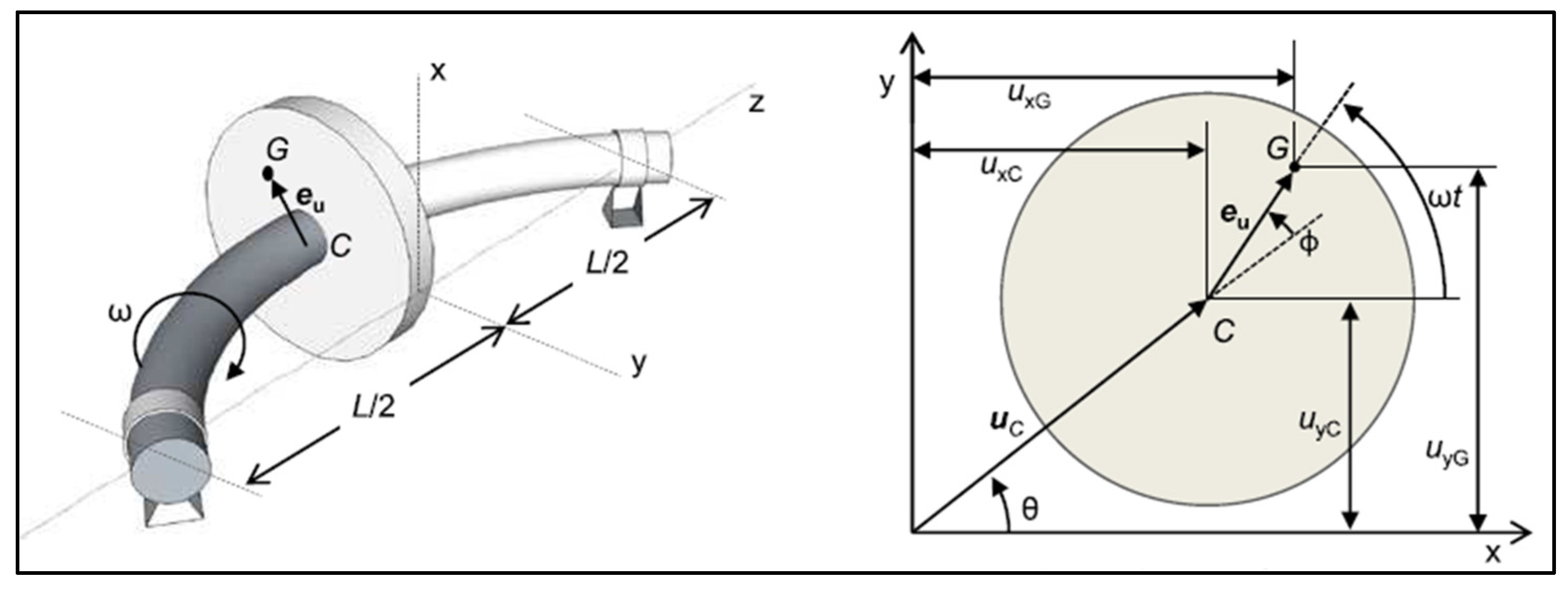Figure 3 shows the unbalance of the disk with respect to its source position relative to the coordinates y and z.

In the figure, the left side, represents the perspective view of the axis supported on the bearing. On the right side, it is the vector representation of the components of the system. The represents the

C

center of the mass axis

m

, and

G

represents the point of unbalanced mass of the disk coupled to the axis, the

e_{u}

is the unbalance vector connected to

C

and

G

. The angular velocity of the axis is ω, and

L

is the length of the axis. The equation of the lateral displacement of the axis with respect to

x

and

y

, can be written as,

(- ω^{2} + 2 i ω ζ ω_{n} + ω_{n}^{2}) U_{x} e^{i ω t} = e_{u} ω^{2} \cos (ω t)

(2)

(- ω^{2} + 2 i ω ζ ω_{n} + ω_{n}^{2}) U_{y} e^{i ω t} = e_{u} ω^{2} s e n (ω t)

(3)

Equation 2 and 3 in complex form can be written as,

(- ω^{2} + 2 i ω ζ ω_{n} + ω_{n}^{2}) u_{c} = e_{u} ω^{2}

. Considere, that rigidity is written as

K_{e} = \frac{48. E . I}{L^{3}}

, which is

E

modulus of elasticity, and the moment of inertia is

I = \frac{π d^{4}}{64}

The natural frequency is

ω_{n} = \sqrt{\frac{K_{s}}{m}} = \sqrt{\frac{48. E . I}{L^{3} m}}

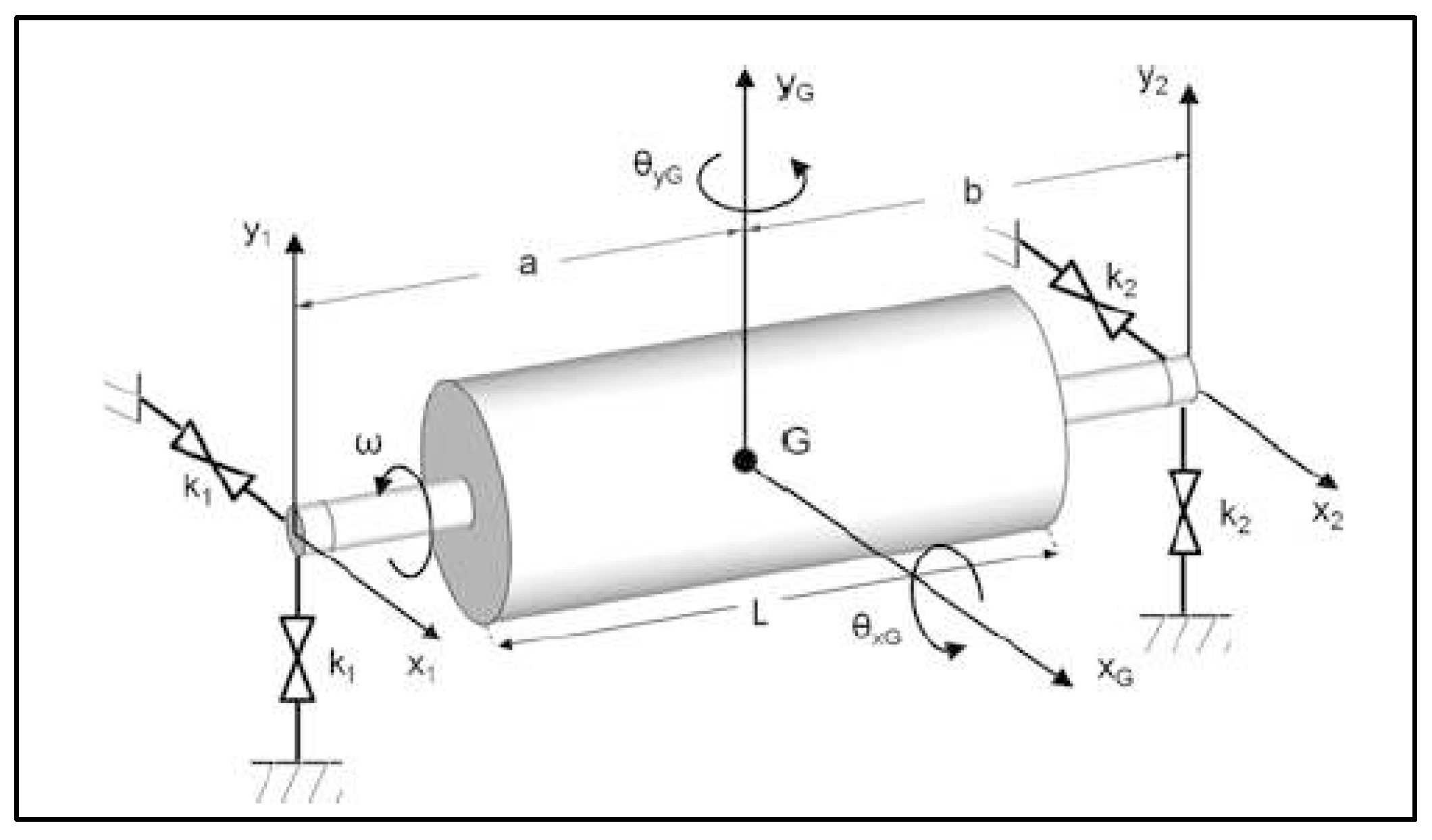
[12; 13]. The equation representing the lateral displacement of the axis coupled with the gyroscopic effect, can be written as,

m {\ddot{x}}_{G} + α x_{G} - γ θ_{y G} = 0

(4)

m {\ddot{y}}_{G} + α y_{G} - γ θ_{x G} = 0

(5)

J_{t} {\ddot{θ}}_{x G} + J_{p} ω {\dot{θ}}_{y G} + γ x_{G} + δ θ_{x G} = 0

(6)

J_{t} {\ddot{θ}}_{y G} - J_{p} ω {\dot{θ}}_{x G} + γ y_{G} + δ θ_{y G} = 0

(7)

The

J_{p}

is the polar rotational moment of inertia

J_{p} = \frac{m R^{2}}{2}

, being

R

the radius of the rotor.

J_{t}

is the transverse moment of inertia (rotational inertia of the perpendicular axis on the same axis of rotation)

J_{t} = \frac{m}{4} (R^{2} + \frac{1}{3} L^{2})

. The

α = K_{1} + K_{2}; γ = - K_{1} a + K_{2} b; δ = K_{1} a^{2} + K_{2} b^{2}

are the stiffness parameters. The

x_{G} = \frac{1}{L} (b x_{1} + a x_{2}); y_{G} = \frac{1}{L} (b y_{1} + a y_{2})

are the lateral displacements. The

θ_{x G} = \frac{1}{L} (y_{2} - y_{1}); θ_{y G} = \frac{1}{L} (x_{2} - x_{1})

represent the rotation of the rotor in

G

[13]. Figure 4 shows the relationship of the arguments of equations 4 to 7.

4. Experimental Methodology

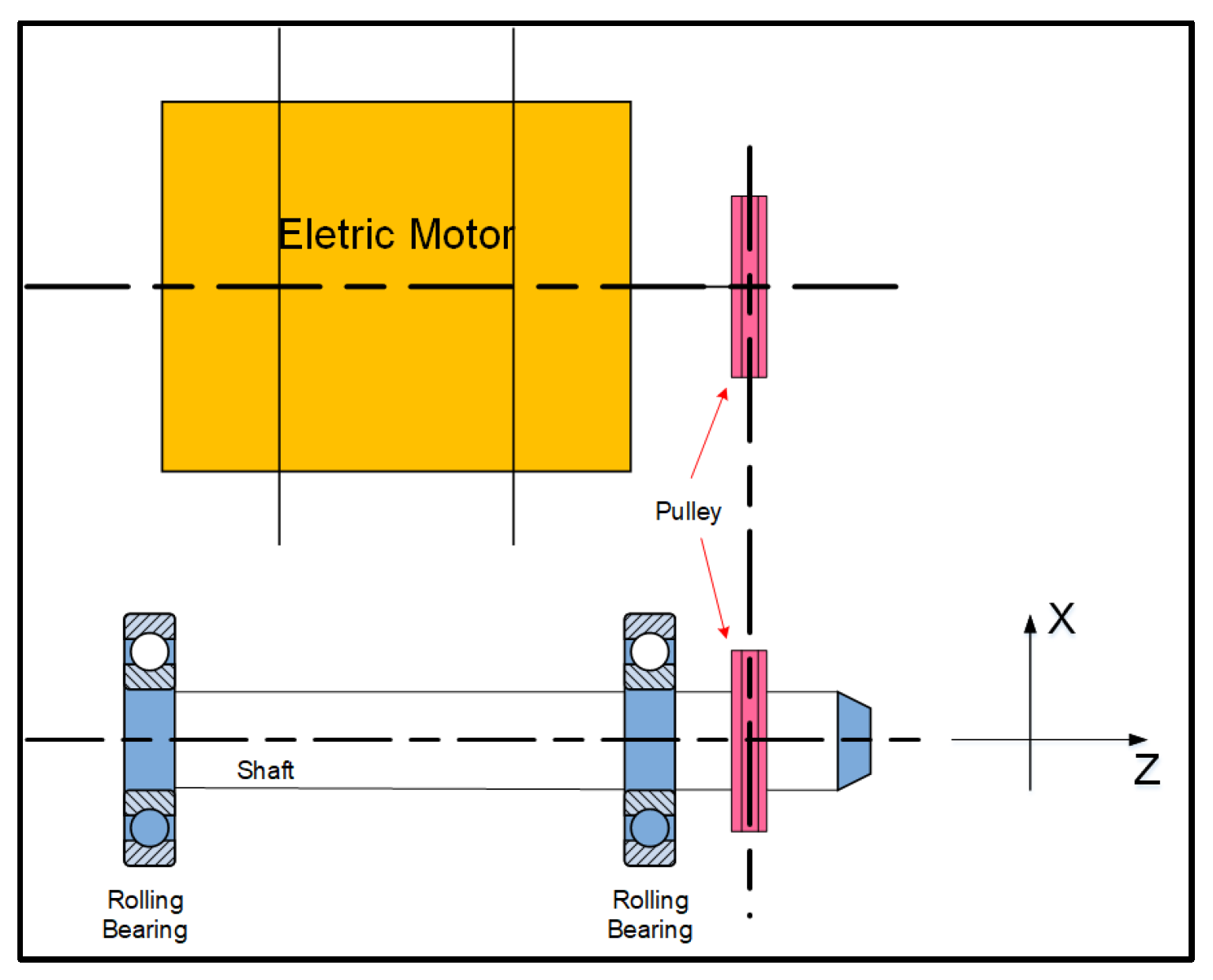
The Jeffcott rotor experiment was set up so that several studies can be developed, the results of which demonstrate the day-to-day physical phenomena of an industry. The process of analysis of the physical phenomena of the experiment contains distinct phases, namely: A) understanding of the dynamic system based on theoretical aspects; B) understanding of the dynamic system based on vibration analysis; C) understanding of the correspondence between the theoretical and practical aspects. From this phase of matching and adhering to existing experimental data, the next process is to develop concepts in which external forces act on the dynamical system that can alter its current state. Figure 5 shows a schematic drawing of the experiment to which the B analysis models will be developed.

The principle of operation, demonstrated in the schematic drawing is simple, the concept is that, when the electric motor starts its operation, transfer the energy to the two pulleys, consequently, develop the rotational movement on the main axis coupled to the two bearing bearings that support it. This whole mechanism is supported on a solid foundation. The elements of this dynamic system are composed of a 1045 steel shaft with mass

m = 0.5 K g

; stiffness of

k = {20.10}^{3} \frac{k g f}{m m^{2}}

; length

L = 120.0 m m

; and diameter of

d = 12.0 m m

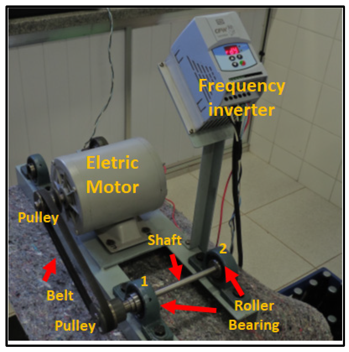
. Two P205 UC205 bearing bearings, both unused (new). An electric motor of 0,5 cv-60Hz; a frequency inverter WEG-CFW10 of 60Hz. The vibration measurement equipment is a VB-8205SD Lutron - frequency range from 10Hz to 1KHz, with vibration sensor sensitivity 15mA DC, meeting the ISO2954 standard [3]. Figure 6 shows the experiment mounted on a bench demonstrating the equipment and elements of the assembly and considering the difference of the bearing bearings between point 1 and 2.

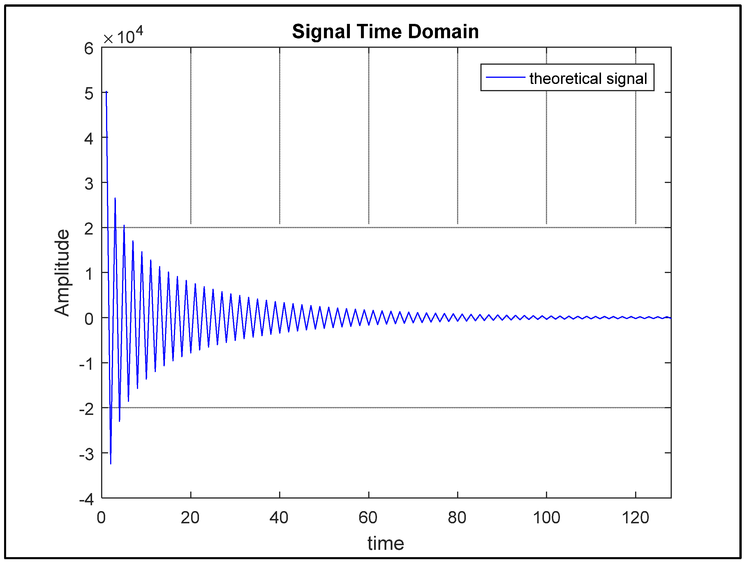
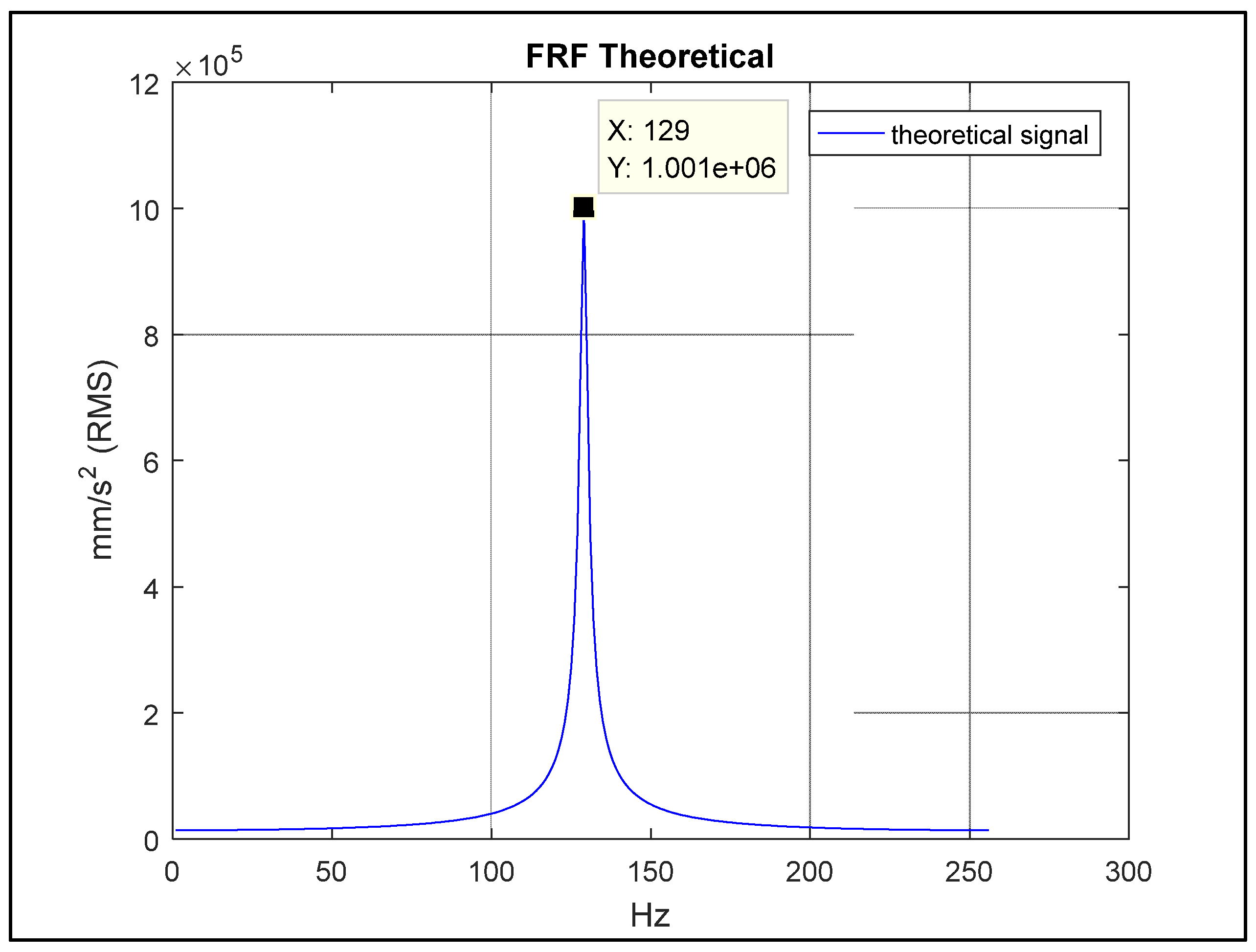
The theoretical model of the system was developed based on the initial conditions of the system, whose Jeffcott theory with its respective equations resulted in the natural frequency response of the system, dampened dynamical system. Figure 7 shows the result of the excitation response in the time domain, using the initial conditions of the system.

Figure 8 shows the frequency domain excitation response (RFF).

After the foundation and development of the theoretical model, the experimental activities were initiated and, thus, the vibration signals of the bearing 1 and 2 were obtained individually in the three axes (x, y and z). Figure 9 shows in detail the positioning of the magnetic-based vibration sensor on the x, y and z axes for the acquisition of the vibration signal.

Note that the reference of the x, y and z axes are positioned in the figure on the left side at the end of the axis demonstrating the bearing measurement. Specifically, the bearings are divided into site 1 and site 2, that is, left and right bearings, respectively. After positioning the accelerometer in the proper place, the signal was captured, allowing the formation of a database of the vibration signal of each bearing, these signals were obtained at the maximum frequency of the motor at 60Hz. 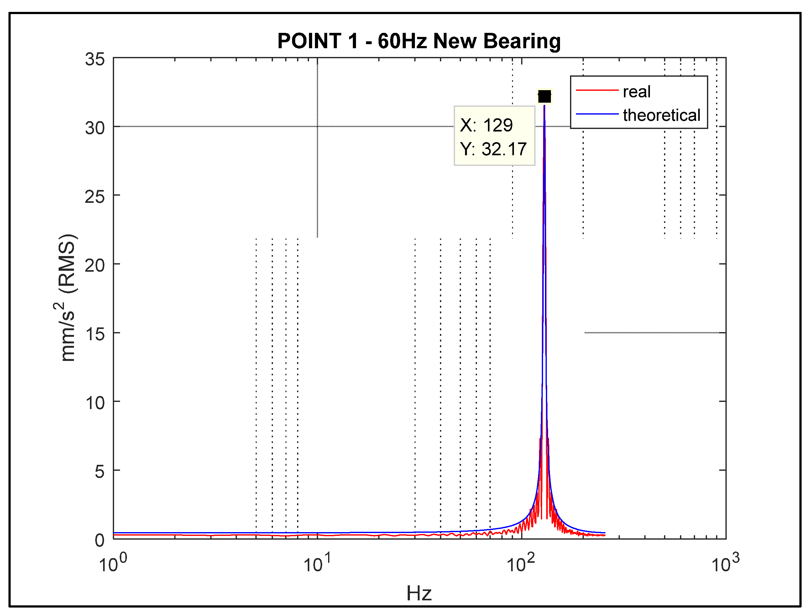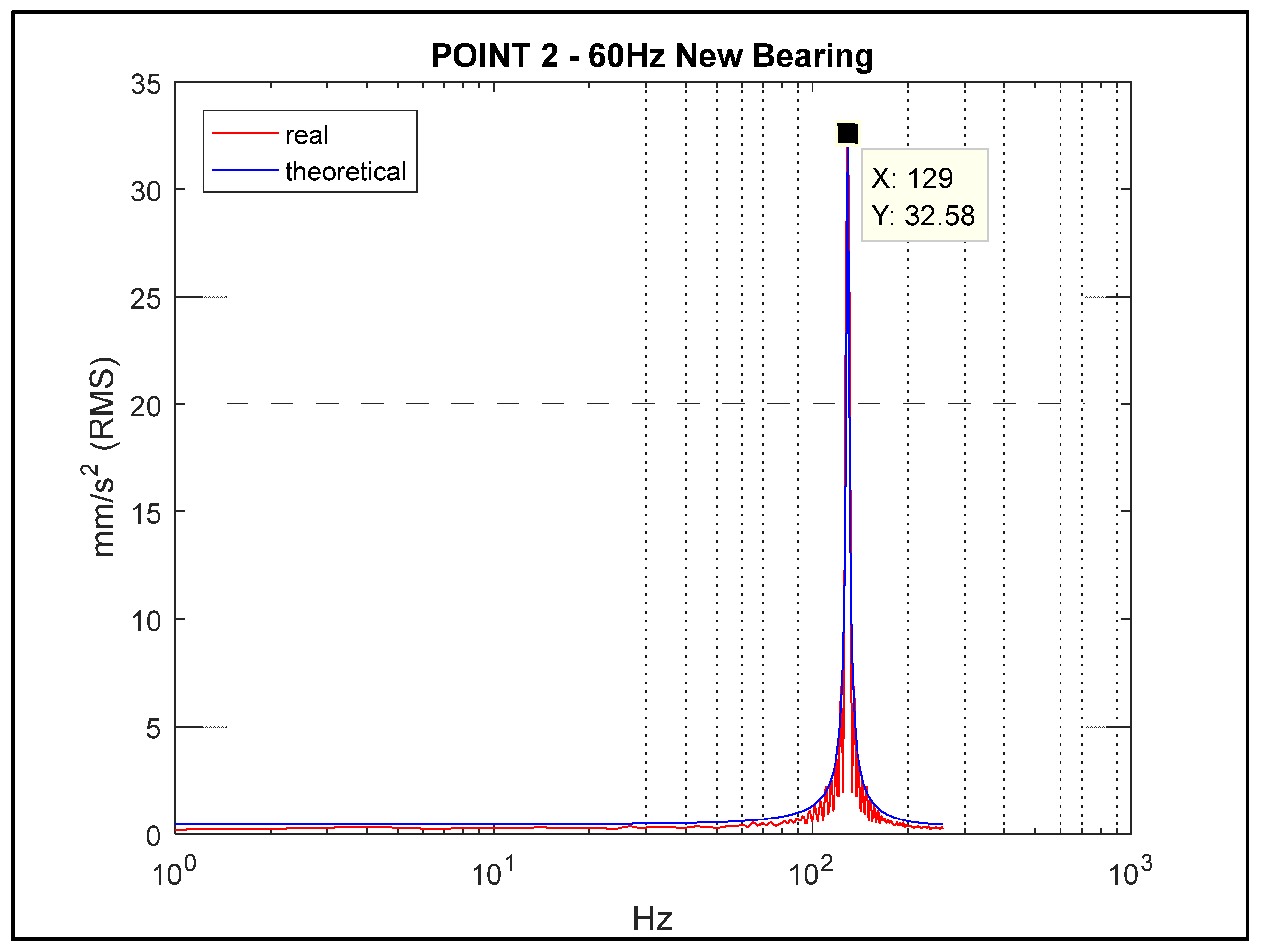A total of 256 variables were collected from each x, y and z axis, in the route mean square RMS condition, forming a vector of 1 x 256, called a vibration signal [3]. The result of this procedure can be seen in Figure 10 and Figure 11, which represent the FRF of each bearing housing.

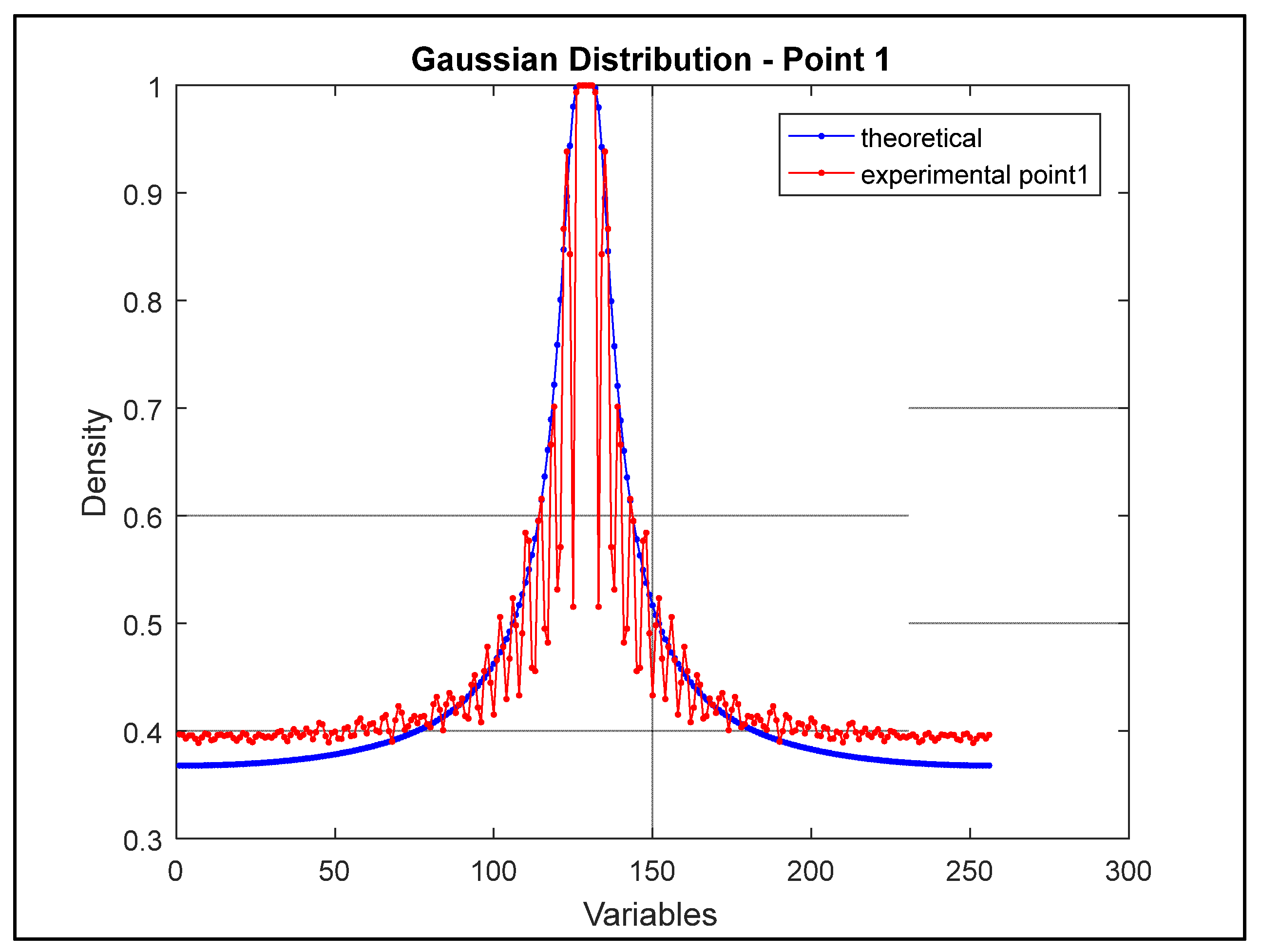
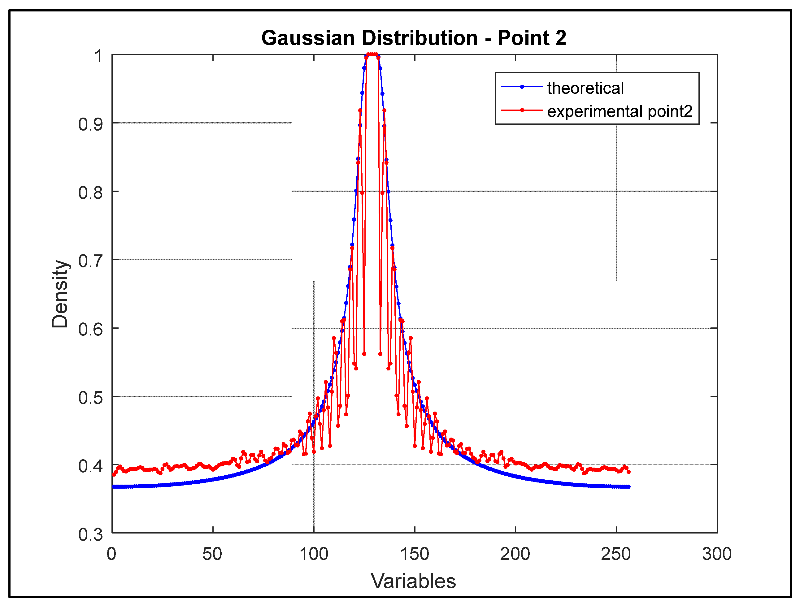
Note that the condition of the position on the frequency axis between the theoretical and experimental vibration signal are similar in both bearing 1 and bearing 2. Based on the finite sample size calculation, to verify whether the sample size of 256 variables allows an acceptable confidence level, a calculation with the confidence level of 95% with an error of 2% was proposed, whose application result demonstrated the need to have 232.3 samples. Therefore, in this work, the size of 256 samples meets the confidence level of 95% with sampling error of 2%. The statistical method was introduced to the work demonstrating the grouping of the signal corresponding to the bearing of point 1 and point 2. Figure 12 and Figure 13 demonstrate the Gaussian distribution of the bearing vibration signals of point 1 and 2 respectively.

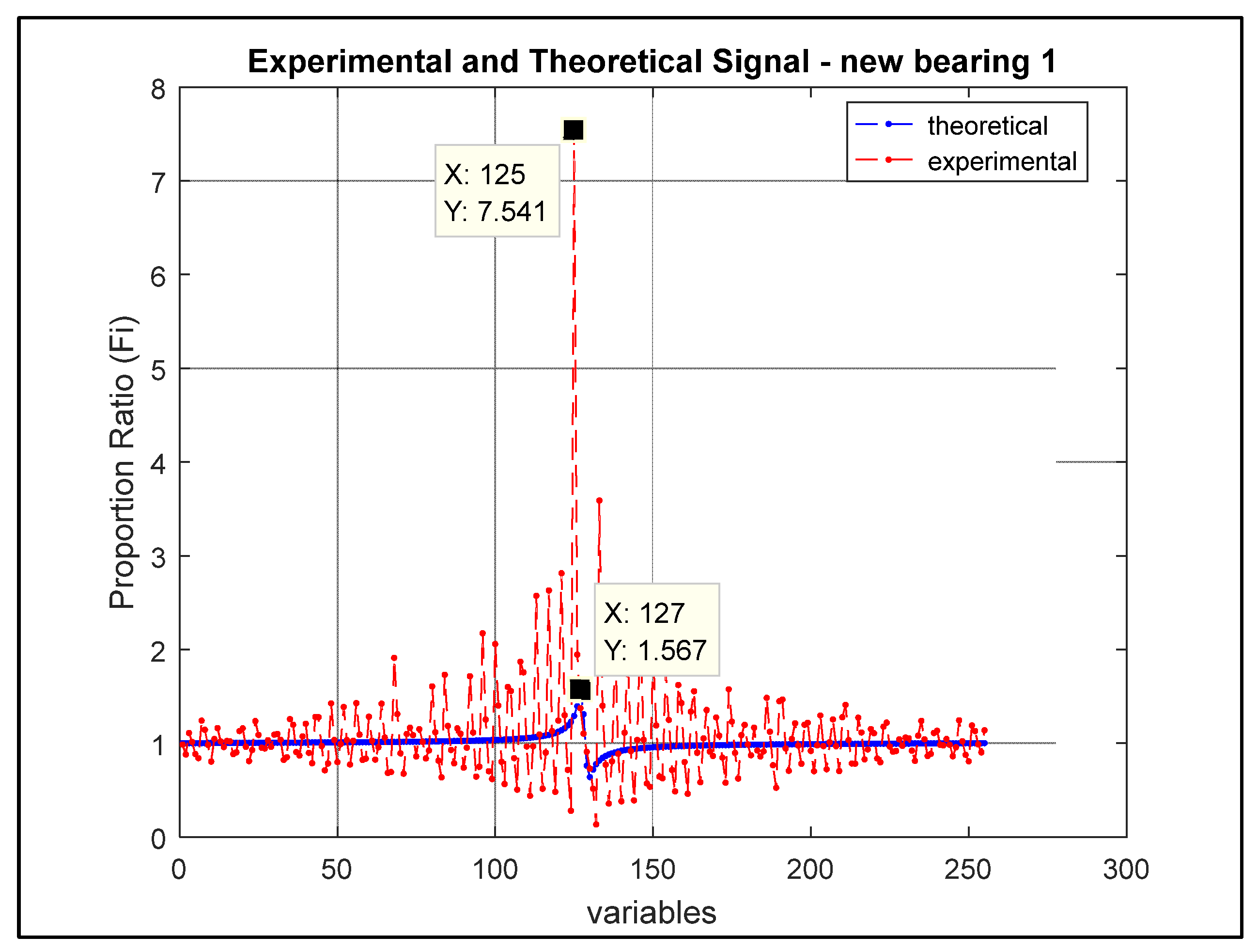
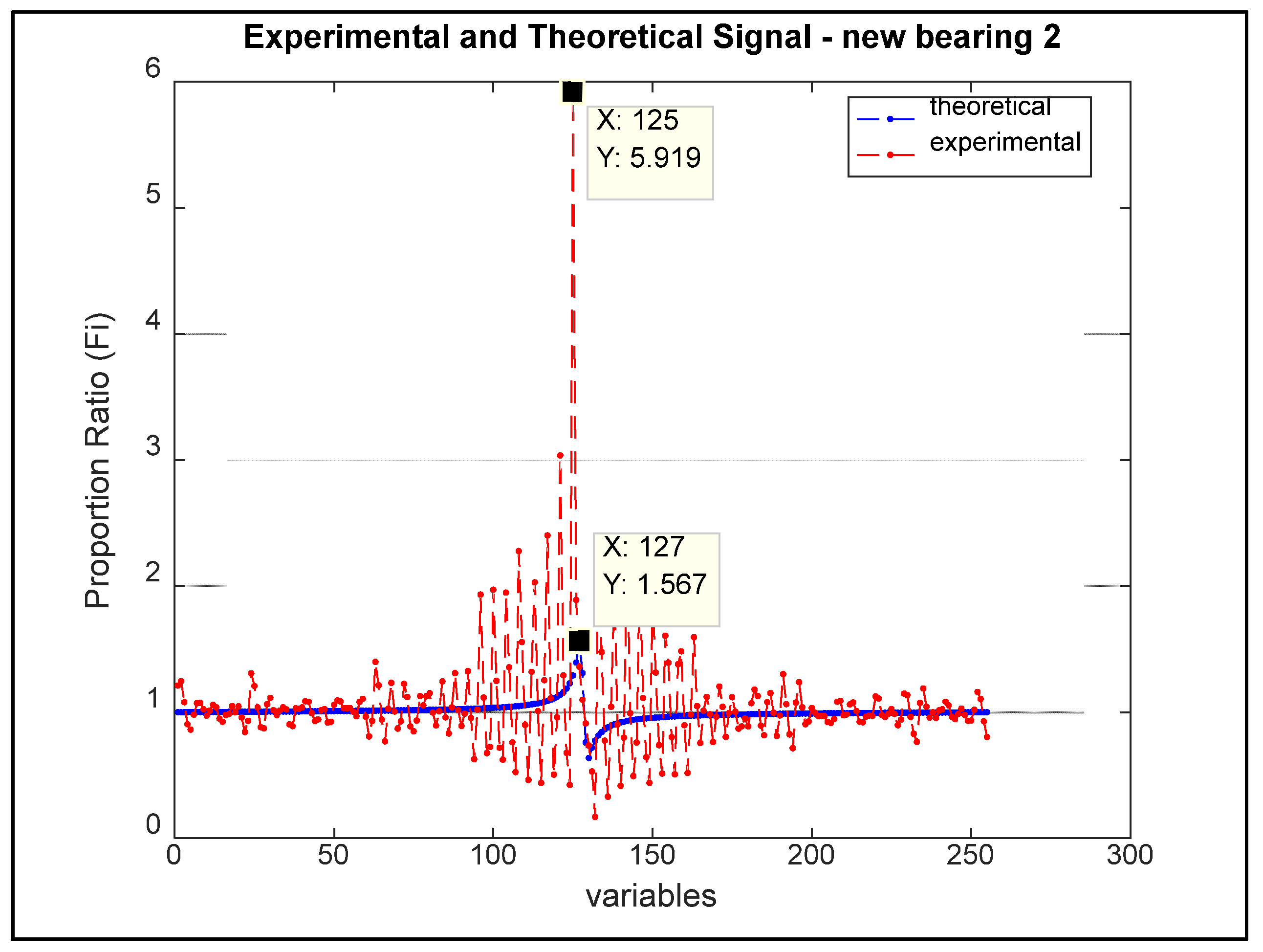
Note that the vibration signals of each bearing correspond in shape with the Gaussian distribution. Subsequently, the application of the Fibonacci theorem for pattern recognition in the vibration signal was developed. Figure 14 and Figure 15 show the relationship of the formation of the concept of pattern recognition based on the location of the value of the natural frequency, in the axis of the variables, of each vibration signal in points 1 and 2.

5. Discussion

This is a work of difficult execution and development, since it involves different methodologies and knowledge. However, the main idea presented here is to form the concept of pattern recognition using Fibonacci theory, applying it to vibration signals from a dynamic rotor. This context meets the condition of a robust design, because, given the severity and problem level of component elements, the pattern recognition can be formed by statistical information extracted from patterns and classify them based on knowledge already acquired [9].

Note that the whole development uses the principle of SHM, with a greater emphasis on pre-processing, whose analogy of the experimental vibration signal to the patterns of the theoretical model demonstrates a great relevance in the similarity of the location of the natural frequency of the system, as shown in Figure 14 and Figure 15. In this case, we observe the importance of this developed context, as being, a principle of validation of a mathematical method, whose result demonstrates the similarity between the values found. Thus allowing to consider the existence of a principle of standard.

Note also that the Fibonacci theorem used in this work is easy to access and use, which allows in many cases linked to industry the development of a direct application, without restrictions or inconsistencies. The contribution to the scientific environment, on the other hand, is to use the model proposed here as a future investigation in other means and foundations that demonstrate the possibility of understanding physical behaviors of a hybrid system. This methodology can be well seen by industrial maintenance engineering, in the aspect of predictive systems, when in the analysis of the useful lifetime, it is possible to understand in a visual way the aspect of a behavior different from the adopted standard.

Currently with the increase of new industrial technologies, the vision for high-impact issues and practical solutions is of fundamental importance.

6. Conclusions

This research paper demonstrates an application of a world-renowned theorem, called the Fibonacci theorem, which was applied to a vibration signal with the intention of obtaining information for the recognition of a pattern. In this case, it is possible to affirm that the proposal was successful and was clearly demonstrated, meeting the main objective of this work.

Therefore, I affirm that this work is complete and can still be successfully inserted in industrial means by the practicality of the mathematical theorem.

Acknowledgments

We thank CNPq and FAPESP for their support and encouragement of the research developed. CNPq - National Council for Scientific and Technological Development (Proc. No. 301401/2022-5). Research Support Foundation of São Paulo - FAPESP (Proc. n. 2023/00861-8).

References

PLATZER, A. , Logical Analysis of Hybrid Systems: Proving Theorems for Complex Dynamics, Berlin, Springer-Verlag, 2010. 457p.
JALALI, M.H. , SHAHRIARI, B., GHAYOUR, M., ZIAEI-RAD, S., YOUSEFI, S., Evaluation of Dynamic Behavior of a Rotor-Bearing System in Operating Conditions, Engineering and Technology International Journal of Mechanical, Aerospace, Industrial, Mechatronic and Manufacturing Engineering, v.8, n.10., 1675-1678p. 2014. [CrossRef]
OUTA, R. , CHAVARETTE, F.R., FARIA, G.A., Comparative Study Of The Dynamics Between Rolling Bearings of a Dynamic Rotor, International Journal of Pure and Applied Mathematics, v.104, n.1, 135-143p. 2015. [CrossRef]
WANG, J. , WEN, H., QIAN, H., GUO, J., ZHU, J., DONG, J., SHEN, H., Typical Fault Modeling and Vibration Characteristics of the Turbocharger Rotor System, Machines, v.11, n.1, p.1-16. 2023. [CrossRef]
MOUCHAWEH, M.S. , Fault Diagnosis of Hybrid Dynamic and Complex Systems, Springer International, Switzerland, 2018. 290p.
ALWAN, M.S. , LIU X., Theory of Hybrid Systems: Deterministic and Stochastic, Springer Nature, Singapore, 2018. 252p.
SWORDER, D.D. , BOYD, J.E., Estimation Problems in Hybrid Systems, Cambridge University Press, Cambridge, 2004. 294p.
BHOWMIK, B. , HAZRA, B., PAKRASHI, V., Real-Time Structural Health Monitoring of Vibrating Systems, Oxon, Taylor & Francis Group, 2022. 249p.
MURTY, M.N. , DEVI, V.S., Pattern Recognition: An Algorithmic Approach, Springer, India, 2011. 276p.
DOUGHERTY, G. , Pattern Recognition and Classification: An Introduction, Springer Science+Business, New York, 2013.203p.
TIANXIN, C. , Perfect Numbers and Fibonacci Sequences, World Scientific, Singapore, 2022. 261p.
LEE, C.W. , Vibration Analysis of Rotors, Korea, Springer Science+Business, 1993. 323p.
YOON, S.Y. , LIN, Z., ALLAIRE, P.E., Control of surge in centrifugal compressors by active magnetic bearings, theory and implementation, Springer London Heidelberg New York Dordrecht, Springer-Verlag London 2013. 292 p.

Figure 1. SHM Utilization Strategy. Source: [8].

Figure 2. Classification Activities for Pattern Recognition. Source: [10].

Figure 3. Generalized Position of the Disk in the Dynamic Rotor. Source: [13].

Figure 4. Decomposition of the Gyroscopic Effect Modeling. Source: [13].

Figure 5. Schematic Drawing of the Dynamic Rotor Experiment. Source: Own Development.

Figure 6. Jeffcott Rotor Experiment. Source: [3].

Figure 7. Response to Excitation in the Time Domain. Source: Own Development.

Figure 8. Frequency Domain Excitation Response. Source: Own Development.

Figure 9. Arrangement of the Magnetic Base Accelerometer in the Bearing Bearing. Source: Own Development

Figure 10. FRF of the Bearing Bearing Vibration Signal 1. Source: [3].

Figure 11. FRF of the Bearing Bearing Vibration Signal 2. Source: [3].

Figure 12. Gaussian Bearing Distribution (Point 1). Source: Own Development.

Figure 13. Gaussian distribution of the bearing (Point 2). Source: Own Development

Figure 14. Proposal of Pattern Recognition by the Fibonacci Theorem. Source: Own Development

Figure 15. Proposal of Pattern Recognition by the Fibonacci Theorem. Source: Own Development.

Disclaimer/Publisher’s Note: The statements, opinions and data contained in all publications are solely those of the individual author(s) and contributor(s) and not of MDPI and/or the editor(s). MDPI and/or the editor(s) disclaim responsibility for any injury to people or property resulting from any ideas, methods, instructions or products referred to in the content.

© 2023 by the authors. Licensee MDPI, Basel, Switzerland. This article is an open access article distributed under the terms and conditions of the Creative Commons Attribution (CC BY) license (http://creativecommons.org/licenses/by/4.0/).

Copyright: This open access article is published under a Creative Commons CC BY 4.0 license, which permit the free download, distribution, and reuse, provided that the author and preprint are cited in any reuse.

MDPI Initiatives

Important Links

Choose an area of interest and we will send you notifications of new preprints at your preferred frequency.

Disclaimer