1. Introduction
Pipelines are critical for the transportation and distribution of liquid and gaseous fuel in various industrial sectors, including oil, gas, and petrochemical. However, these pipelines have been laid across diverse and often harsh terrains, making it challenging to maintain their structural integrity. To safeguard national security and economic growth, it is important to study and develop comprehensive monitoring methods that can detect and mitigate external threats, such as sabotage, unauthorized access, construction accidents, and natural disasters, as well as internal structural degradation caused by various factors such as corrosion, erosion, fatigue, and material degradation due to environmental and operational factors.
Different technology-driven and human-operated evaluation programs have been employed to protect pipeline infrastructure for many years. Currently, structure health monitoring (SHM) is a novel technology that integrates sophisticated sensor systems with intelligent algorithms to assess “health” of a structure. This approach has the potential to enhance reliability and safety, optimize performance, increase automation capabilities, and decrease overall lifecycle costs. As such, SHM has garnered significant interest in recent years and is now recognized as a promising solution for improving the structural integrity of civil infrastructure, aerospace, and mechanical systems. In these applications, damage detection by guided-wave nondestructive testing has attracted widespread interest. Ultrasonic sensors can detect the backscattering acoustic response, which provides data for identifying different events, such as structural damage, or changes in the structure, like the addition of clamps or the presence of welds within the structure.
Elastic perturbations known as guided waves are capable of propagating over extended distances in thin-walled structures while experiencing minimal amplitude loss. Laboratory experiments [
1] have demonstrated the efficiency of using guided acoustic waves to detect and locate pipeline anomalies in critical areas that are susceptible to defects. To excite a cylindrical structure and propagate UGWs, an appropriate signal is chosen, which will then propagate through the structure and encounter any damage or other material discontinuities. Traditionally, by analyzing the resulting changes in the waveform, the location and severity of the damage can be quantified. It is important to note that UGWs can experience dispersion as they propagate, which can affect the accuracy of damage detection. To analyze the dispersion of UGWs, a MATLAB toolbox package named PCDISP [
24] is commonly used. This toolbox utilizes Navier Lame's equation [
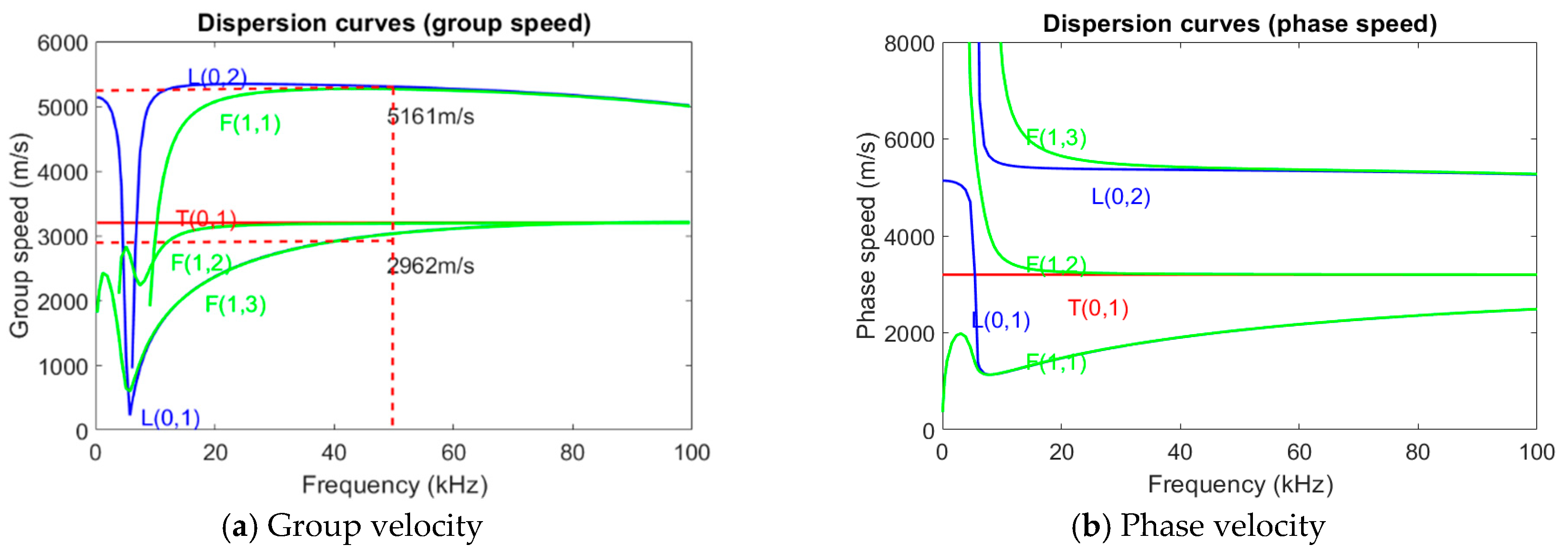
19], which describes the behavior of elastic waves in solid bodies, to calculate the dispersion curves of different guided wave modes. The use of PCDISP allows for a more accurate analysis of the dispersion and ultimately a more accurate identification of the location and severity of the damage. By utilizing the appropriate excitation signal, analyzing the resulting changes in the waveform, and utilizing tools such as PCDISP, it is possible to effectively detect and quantify damage in the structure. Wave phase velocities and group velocities of a steel pipeline with an outside diameter of 12 inches and wall thickness of 0.5 inches are shown in
Figure 1a,b.
Also, guided wave NDE has potential to significantly decrease the number of sensors necessary for monitoring a structure. Specifically, guided wave NDE technology is a promising method for structural health monitoring (SHM), but one of the main limitations is the size, cost, and practical constraints of deploying conventional NDE sensors ubiquitously. In guided acoustic wave sensing, the exciting transducer is therefore typically also used as the measurement sensor, thereby measuring the backscattered acoustic wave. Such an installation scenario can be highly limiting in terms of investigating damage over large distances and in remote locations, and the amount of information that can be extracted is also limited by what can be measured at the excitation location. The use of distributed fiber optic sensors as alternative measurement transducers has been proposed as an alternative solution, and they can be placed at multiple points along a pipeline to monitor for damage. Practical limitations of permanently mounting conventional NDE sensors on structures have been widely discussed [
2]. Assuming sufficiently high frequency bandwidth can be achieved, distributed fiber optic sensors are promising candidates for guided acoustic wave detection schemes because they are able to detect acoustic signatures generated by external events or alternatively scattered by defects within a pipeline segment with high spatial and temporal resolution [
3,
4,
5].
In the past decades, distributed fiber vibration/acoustic sensor technology has gained increasing attention and tremendous growth. The quasi-distributed/point fiber vibration/acoustic sensor technologies include fiber Bragg grating (FBG) [
3], Fabry–Pérot [
4], and Multimodal interference [
5]. Various interferometric configurations include; the Sagnac interferometer [
6], the Mach–Zehnder interferometer (MZI) [
7], and polarization-OTDR (POTDR) [
8]. Fiber optic sensors are known for being resilient in harsh environments and capable of distributed interrogation. They have a unique ability to perform distributed strain, and acoustic measurements using backscattered light phenomena in unmodified telecommunications fibers or fibers that have been modified to enhance the scattering, resulting in high sensing performance with improved spatial resolution measurements [
9,
10]. The most common distributed acoustic sensing modality involves a technique referred to as phase–optical time domain reflectometry (φ – OTDR) as discussed in our recent review of distributed optical fiber sensing [
11]. The Φ-OTDR system utilizes the interference effects within pump pulses generated by a narrow linewidth (usually <10 kHz) laser source. The Φ-OTDR system demodulates the backscattered Rayleigh signal amplitude/phase to acquire acoustic signals. The Rayleigh signal amplitude varies with the strain on the sensing fiber induced by the surrounding acoustic signals. In the use of a fiber-optic-based distributed acoustic sensing (DAS) system, the fiber-optic cable is used as the sensor; in which a pulsed laser is used to excite the fiber and backscattered light is detected and processed using appropriate optical interrogator hardware.
However, the limitation behind the traditional guided wave based NDE technology is that the number of transducers is limited and typically located at the source of the ultrasonic guided wave. Currently, for raw data acquired based on fiber acoustic sensing, machine learning (ML)-based data analysis techniques can offer advantages in classification, pattern recognition, prediction, and system optimization, especially when there is no explicit mathematical model to describe the relationship between inputs and outputs [
12]. A great deal of research has been pursued seeking to improve the dynamic range, spatial resolution, and sensitivity of the DAS system hardware and signal processing methods. However, the ability of event recognition is typically the goal when considering the limitation of performance in field application. High nuisance alarm rates can occur due to complex environmental interferences and benign artificial disturbances, leading to false alarms. To address this, signal feature extraction methods have been proposed to accurately identify the events [
13]. Feature-based methods can achieve high recognition rate if carefully implemented but require careful feature selection and relatively complex real-time processing to extract signal features. Different disturbances also cause unique effects in spatial and temporal domains. In their work, Sun and colleagues [
14] proposed a method for recognizing events through the extraction of morphological features from a time-space data matrix. They employed correlation techniques to classify three distinct events, namely manual excavation, walking, and vehicle passing.
A key barrier to the wide adoption of machine learning based data analysis for SHM, is that the procurement of training datasets of damage/failure events of real-world structural system of interest are both expensive and time consuming. While it is relatively straightforward to gather data for events such as humans walking or vehicles passing, obtaining real-time sensor data for pipeline structural damage or failure events is exceedingly challenging. Further, pipelines can undergo a wide variety of damage events, further complicating ML model training and degrading ML model performance.
This challenge can be addressed by training ML models on simulated sensor datasets. Such simulations fuse (i) a sensor measurement model (e.g., distributed acoustic sensor measurement model) with (ii) a high-fidelity physics-based numerical model simulation of the structural degradation event (e.g., ultrasonic vibrations of a pipeline with corrosion damage). Hence, the high-fidelity numerical model response is filtered through a suitable sensor model to simulate sensor measurements. This simulation strategy can be systematically deployed to simulate sensor datasets for various pipeline degradation events. Next, an ML classifier can be trained on these diverse and rich simulated datasets to predict structural degradation events of interest. The ML classifier can further be improved by supplementing training data with available experimental measurements. This concept is known as domain adaptation in ML literature and is increasingly adopted in SHM [
15].
In this paper, we propose a CNN-based classification method that directly uses a time-space data matrix for the full distributed sensor system. Deep learning, specifically Convolutional Neural Networks (CNNs), has shown superior performance over traditional machine learning (ML) algorithms in many applications, including pipeline structural health monitoring (SHM) and defect identification using distributed acoustic sensing (DAS) data. The use of CNNs in combination with DAS systems can greatly enhance the accuracy of SHM by providing real-time data analysis for detecting and identifying defects in pipelines. Unlike traditional ML algorithms, CNNs can automatically extract features from raw data and identify patterns that are difficult for humans or conventional algorithms to recognize. This capability is particularly beneficial for processing large amounts of data generated by DAS systems in real-time. CNN-based SHM systems can also adapt to changing conditions and automatically adjust their parameters to optimize performance, making them well-suited for complex environments where conventional approaches may be less effective. In summary, the use of CNNs in combination with DAS systems have the potential to significantly improve pipeline SHM and defect identification by providing accurate and timely analysis of large amounts of sensor data [
12].
The datasets used in this study were generated through finite element simulation of guided wave propagation on the surface of a pipeline, which included various types of damage severities and shapes relevant to common corrosion modes in pipelines. The simulations also incorporated varying levels of noise to emulate real-world conditions during sensor deployment. Our objective was to develop a comprehensive learning framework for guided-wave-based damage recognition, covering the entire process from dataset collection to feature extraction and selection. For model training and prediction, we utilized a Convolutional Neural Network (CNN) algorithm. In this study, various CNN models with different structures and activation functions will be considered to test the prediction performance under diverse configurations. The focus of the study is not on the specific architecture of the model, but rather on demonstrating the effectiveness of the overall learning framework in processing simulated sensor data and building machine learning models for pipeline damage recognition. By exploring different CNN architectures, we aim to understand how the choice of model structure and activation functions may impact the performance of the learning framework for this particular application.
4. Event Recognition
4.1. Comparison of Common CNNs
Convolutional neural networks (CNNs) have gained significant popularity in recent years due to their remarkable effectiveness in processing and classifying signals, such as time-series data from sensors or audio signals. This can be attributed to the unique ability of CNNs to capture local patterns and time dependencies in the input data while maintaining robustness to changes in the timing and amplitude of the signal. As a result, they are particularly well-suited for processing complex and noisy signals that are frequently encountered in real-world applications.
In this study, our primary objective is to compare the performance of various CNN models in the task of classifying pipeline signals into six distinct categories using a relatively small dataset. To accomplish this, we considered three crucial variables in our CNN models: the number of layers, kernel size, and activation function. Specifically, we trained six different CNN models with either 1 or 2 layers, a fixed kernel size of 10, and one of three activation functions: "relu", "sigmoid", or "tanh", as presented in
Table 4.
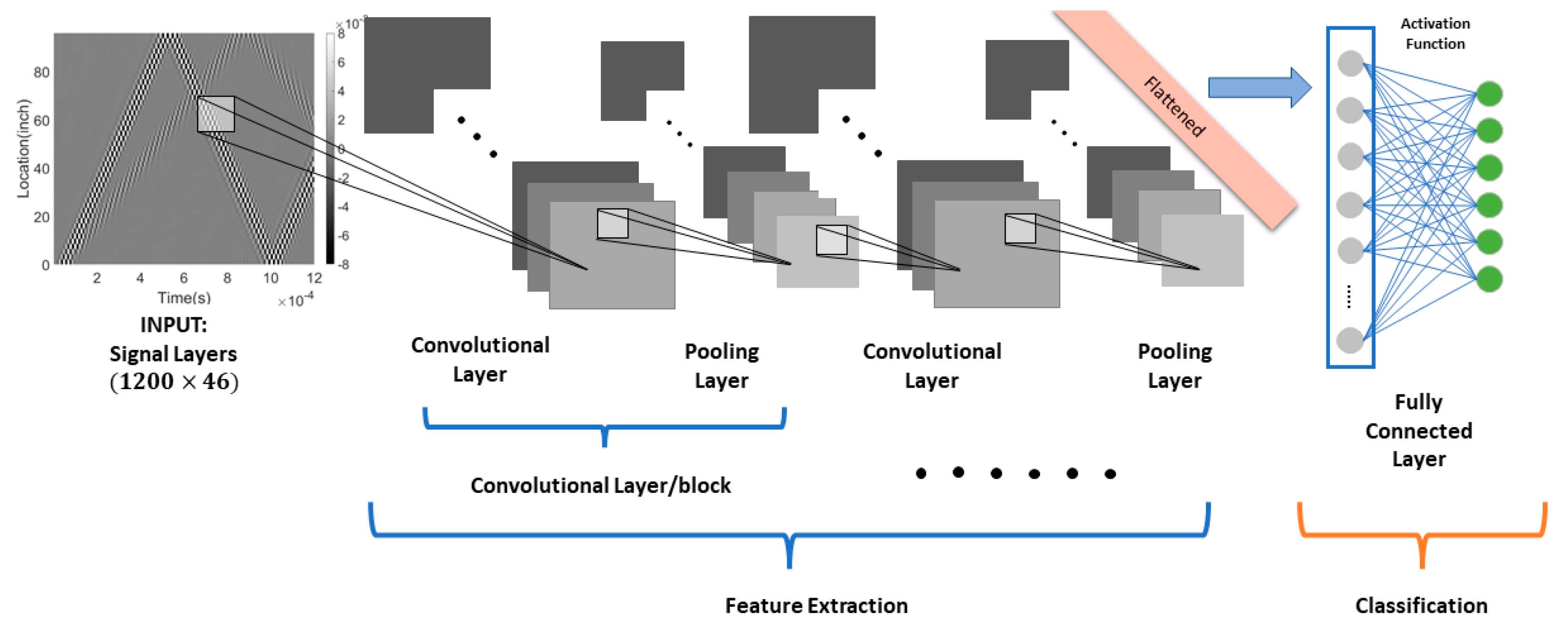
In
Figure 11, we showed an example as one of these CNN model candidates, which is a relatively shallow CNN architecture for classifying signals based on their waveform patterns. As mentioned above, our dataset consists of 150 samples, each with dimensions of 46 (space) x 1200 (time points), and no noise interference. While the dataset may be limited in size, we adopted a systematic approach to ensure reliability and validity of our results, accounting for constraints imposed by available data. First, we carefully pre-processed the dataset, normalizing the input features and removing any potential outliers or inconsistencies. To account for the small dataset size, we employed a stratified sampling approach to maintain the distribution of the six different types of pipeline signals when splitting the data into training and testing sets. In order to account for potential variations in model performance due to random initialization and other factors, we repeated the training process for each CNN model using a large number of iterations (1000) to strike a balance between computational feasibility and reliable performance estimation. This allowed us to observe the distribution of prediction accuracy across multiple runs, providing a robust estimation of each model's performance. Additionally, we employed cross-validation techniques, such as k-fold cross-validation, to further ensure the generalizability of our results, given the limited dataset size. This approach helps to mitigate the risk of overfitting and provides a more reliable estimation of model performance.
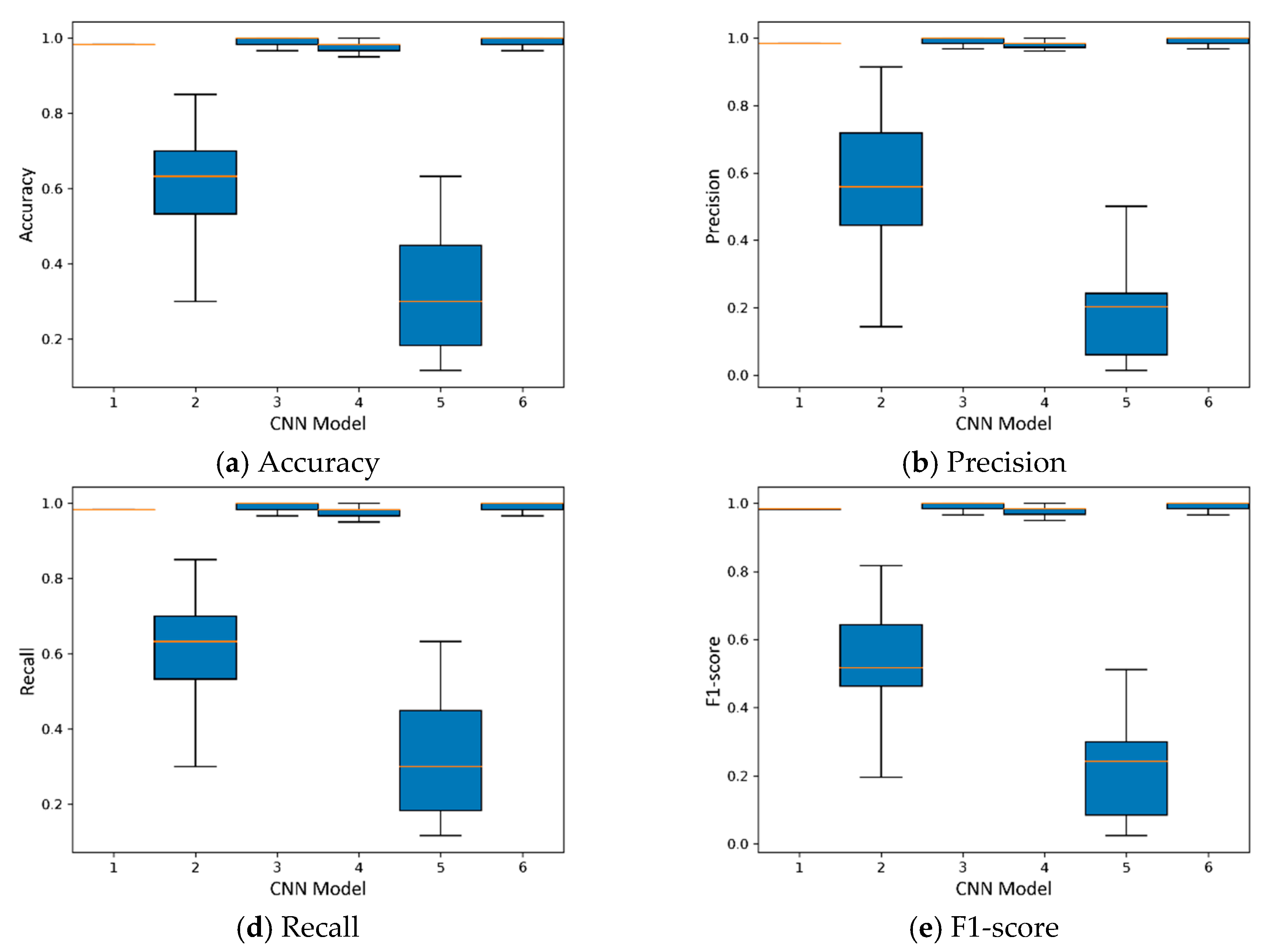
To ensure the reliability of our findings, we repeated the training process 1000 times for each model to examine the distribution of prediction accuracy.
Figure 12 shows the prediction accuracy distribution for each CNN model. Our results showed that among the 6 CNN models tested, K-fold iteration test of model 3 and model 6 shows good robust properties and high accuracy. Here, we select CNN model 3, which is the one with 1 layer, kernel size of 10, and 'tanh' activation function. This CNN model consistently achieved the highest test accuracy across multiple repetitions of the training process.
4.2. The Impacts of classification accuracy due to sensing system to the Robustness of Data Classification
In this section, we compare the classification accuracy of two different acoustic sensing systems: a fully distributed acoustic sensing (DAS) system and a quasi-distributed acoustic sensing (qDAS) system. The DAS system provides continuous measurements along the entire length of the pipeline, while the qDAS system uses a limited number of sensors placed at discrete locations along the pipeline. We evaluate accuracy of these systems in classifying the condition of the pipeline based on six different defect types. It is noted that fully distributed sensing capability is currently limited for ultrasonic guided wave acoustic monitoring due to both the large gauge length in current standard commercial systems (~1m) and the limited acoustic frequency bandwidth (~10kHz). Nevertheless, we include hypothetical fully distributed sensing schemes for completeness.
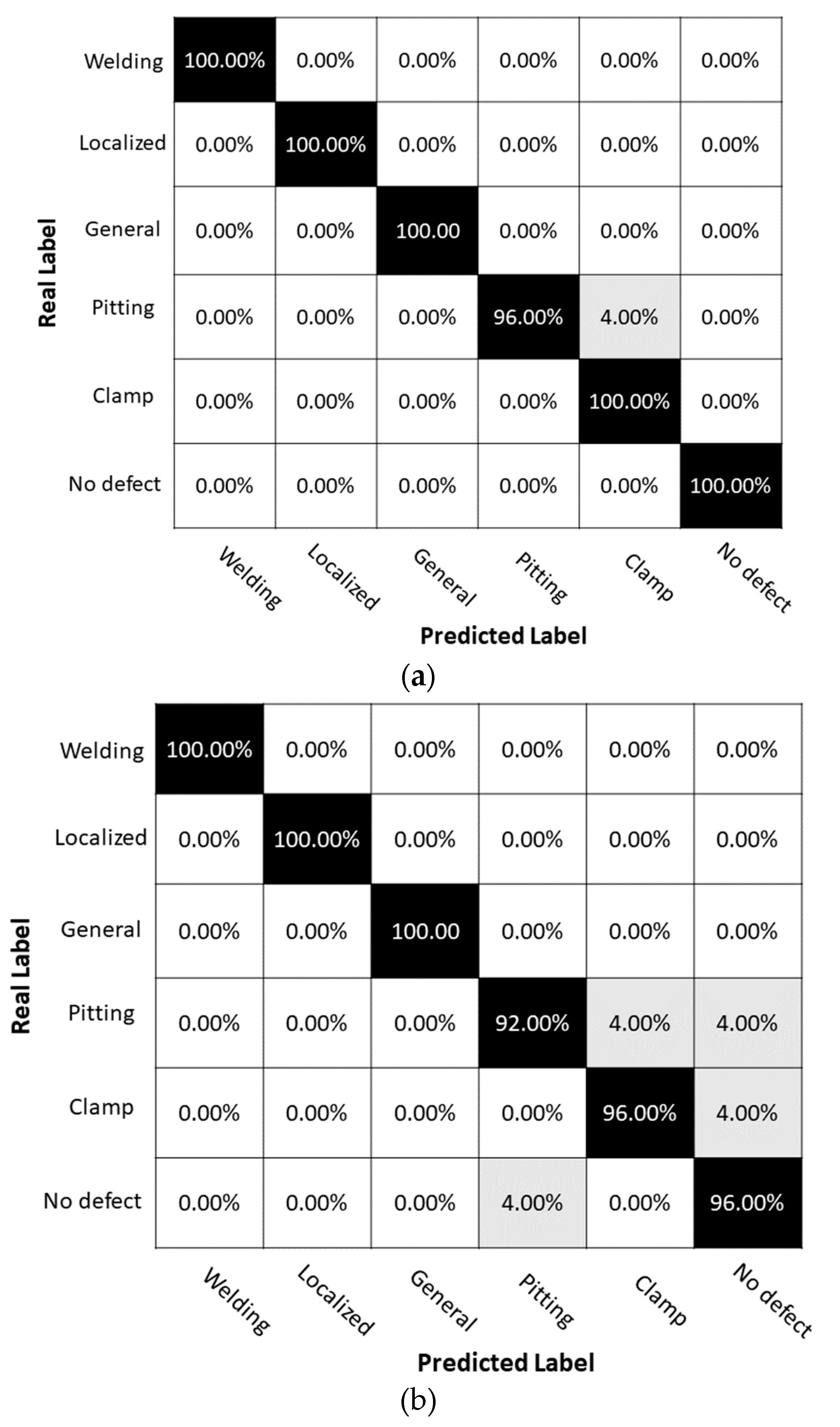
The confusion matrix and classification report for the DAS system without introduced noise indicates near-perfect accuracy for all defect types, with an overall accuracy of 99%. This suggests that the DAS system is highly effective in capturing the subtle differences in acoustic signals associated with different types of pipeline defects and can reliably classify the condition of the pipeline. However, limitations of existing DAS system prevent realization of such a distributed sensor network in practice.
In contrast, the confusion matrix and classification report for the quasi-distributed system indicate a slight reduction in accuracy across different defect types, with an overall accuracy of 96%. Specifically, in
Figure 13, the system performs well in detecting general corrosion, localized corrosion, and weldings, but shows lower accuracy for clamps and pitting corrosion, which is likely due to the weaker associated scattering amplitudes and the relatively small spatial extent. Overall, these results suggest that the choice of sensing system can have a significant impact on accuracy of pipeline defect classification, with fully distributed systems providing higher accuracy compared to a quasi-distributed system in case of sensors without introduced noise. Sensor network optimization subject to realities of available performance of existing and emerging DAS and qDAS systems is an important topic for further investigation in future studies.
The results of the confusion matrices based on the fully distributed acoustic sensing system and the quasi-distributed acoustic sensing system show high classification accuracy for all pipeline features, as shown in
Figure 13 and
Table 5. Both systems correctly classified welding, localized corrosion, general corrosion, and no defect features with a precision and recall of 1.0. However, the results for pitting corrosion are lower than for other features, especially in the quasi-distributed sensing system, which has a recall of only 0.92. This can be attributed to the relatively weak amplitude of acoustic scattering associated with pitting corrosion and need for careful meshing to accurately capture this feature. It is essential to consider spatial resolution and sensitivity of sensing systems when detecting subtle features like pitting corrosion for accurate classification.
In summary, the results demonstrate the high classification accuracy of both fully distributed and quasi-distributed acoustic sensing systems for various pipeline features. While both systems show similar performance in detecting most types of defects, the detection of subtle features like pitting corrosion requires careful consideration of the modeling strategy in simulation and the spatial resolution of the sensing system.
4.3. Analysis of Classification Performance with noise effect
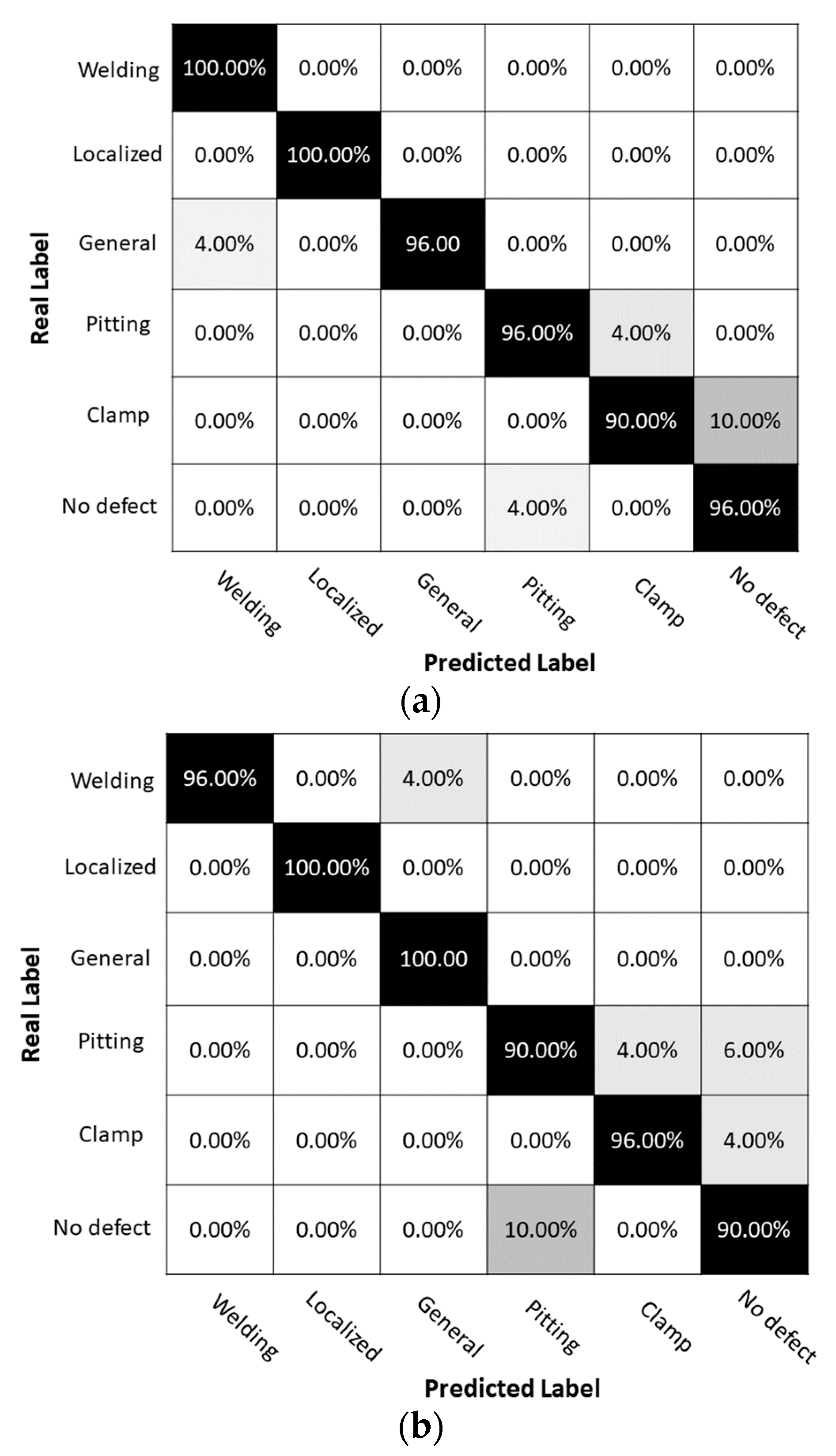
In this scenario we introduce noise, and again present two confusion matrices and classification reports for a fully distributed sensor system and a quasi-distributed sensor system (
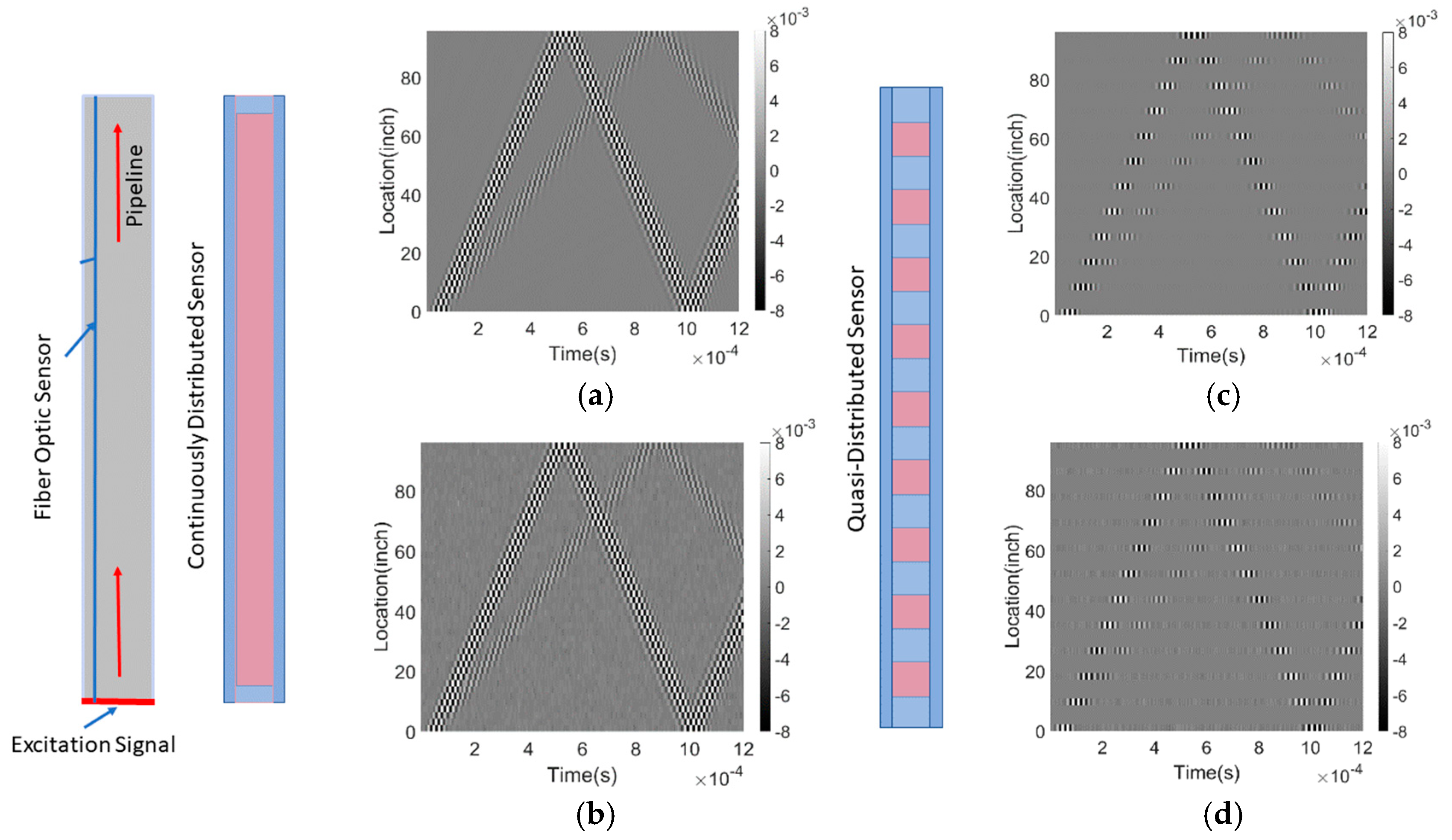
Figure 14). Sensor systems are affected by Gaussian noise with a signal-to-noise ratio of 9.63dB. The training dataset for CNN model is shown in
Figure 9c,d.
The confusion matrices and classification reports show performance of sensor systems in classifying six different types of defects in a pipeline condition monitoring application. Comparing two confusion matrices, it is evident that the fully distributed system has a higher overall accuracy of 98% compared to quasi-distributed system's accuracy of 96%. This result is consistent with the fully distributed system demonstrating a higher precision and recall for most of the classes. For example, in
Figure 14 and
Table 6, the fully distributed system has a higher recall and precision for welding, localized corrosion and pitting corrosion, indicating that it correctly classified all instances belonging to those classes. In contrast, the quasi-distributed system has lower recall values for these classes, but there is improved performance for localized corrosion, general corrosion, and clamps. The fully distributed system also demonstrates a higher precision and recall for pitting. On the other hand, the quasi-distributed system showed improved performance for localized corrosion and general corrosion, which could be due to introduced noise affecting the fully distributed system more significantly than the quasi-distributed system. Detailed investigations of various sensor networks and configurations is an important aspect of optimizing the performance for a particular sensing objective of the sensor system.
4.4. Analysis of Classification Performance with noise and varying quasi-distributed sensing
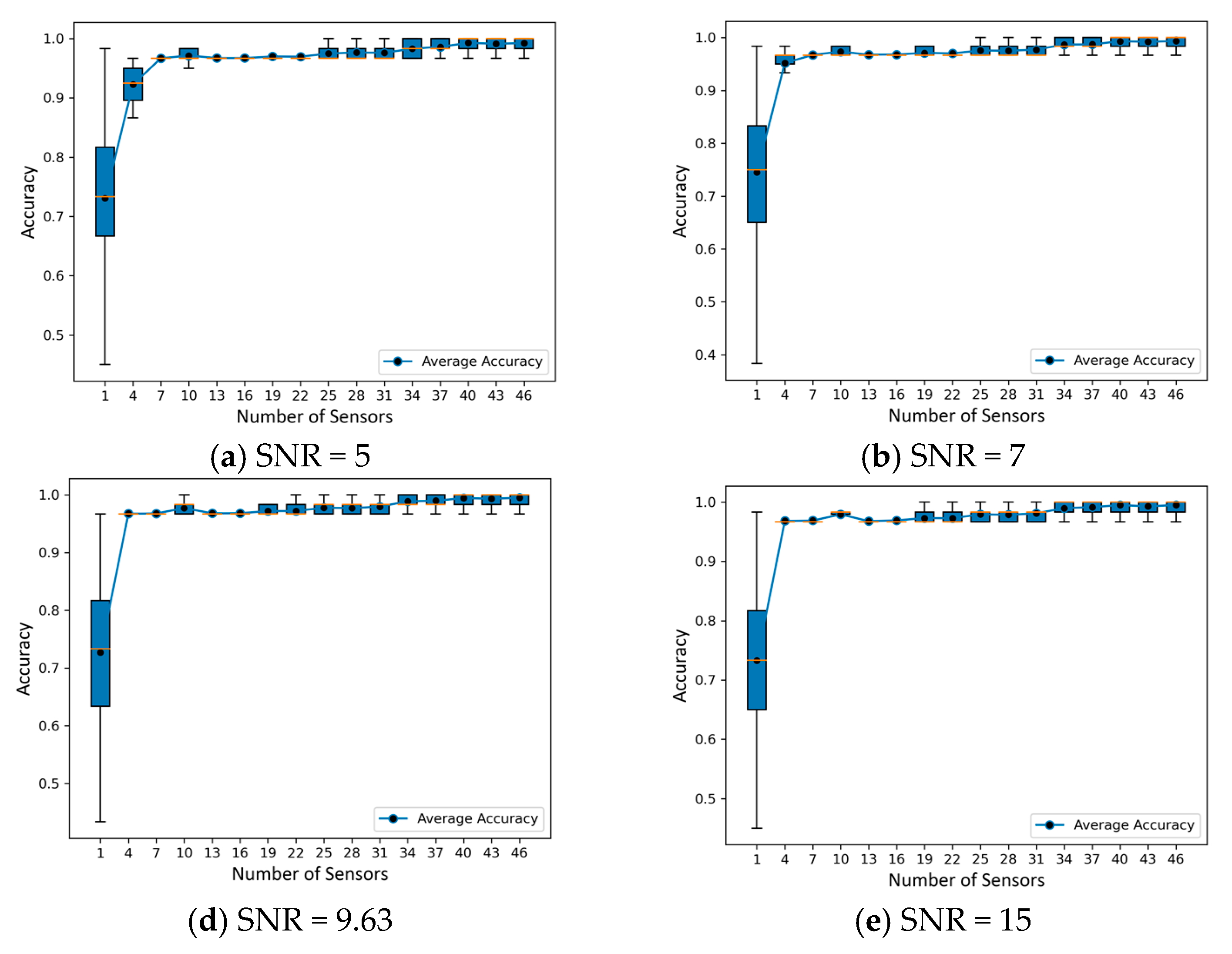
In this study, we have explored the performance of quasi-distributed acoustic sensing systems compared to fully distributed systems. Quasi-distributed systems utilize a limited number of strategically placed sensors to provide a balance between performance and resource utilization. We conducted a comprehensive analysis of the prediction accuracy of quasi-distributed systems at different sensor configurations, investigating the impact of sensor segments on prediction accuracy.
To investigate the machine learning classifier based on ultrasonic guided acoustic wave and fiber optic sensor fusion in more detail, we consider the possibility of varying positions and number of quasi-distributed sensors, which can be adjusted as shown in
Figure 15 as red segments of 1, 4, 7, 10, 13, …,40, 43,46 (Continuous DAS) at an assumed noise level (SNR = 9.63dB). The configuration shows a fiber sensor that completely covers the pipe with measurement units evenly distributed along its length. To evaluate their performance, a series of tests were conducted, and the results are presented in
Figure 16 and described in more detail below.
In addition to the total sensor segment numbers, we also explored the effect of sparse sampling on the acoustic sensing system's ability to withstand variations in sensor positioning. To evaluate the influence of sensor positioning at varying signal-to-noise ratios, we uniformly selected sensor segments for a specific sensor count and carried out the selection procedure 10000 times at a consistent noise level. We examined 16 distinct sensor numbers, ranging from 1 to 46, with sparse sampling playing a role in this selection. By creating boxplots of the dataset, we could visually appraise the distribution of prediction accuracy across various SNR and sensor numbers.
These visualizations offer insight into the performance fluctuations for each configuration and the system's ability to withstand alterations in sensor placement, with sparse sampling potentially contributing to the observed variations.
Figure 16 shows the impact of randomly down spatial sampling of received signals on classification prediction using a CNN under various levels of background noise. Our results demonstrate that as the level of background noise increases, the prediction accuracy becomes less stable, with an increased variance and more outliers. Furthermore, as the sampling size increases, the diversity of random sampling decreases, thereby improving the robustness of multiple predictions. However, increasing the spatial size of the sampling from 16 to 46 sensor segments did not significantly improve prediction accuracy, and in some cases, a specific small subset of the training set achieved higher accuracy than a fully sampled (46 sensor segments) training set.
Our findings reveal a trade-off between the number of sensor segments and prediction accuracy in the context of sparse sampling. However, this improvement becomes less significant as the number of sensors rises. Engineers can effectively tailor the design of quasi-distributed acoustic sensing systems for diverse applications by considering the signal-to-noise ratios and the number of sensors to achieve an optimum between predictive accuracy and reduced system intricacy and resource requirements using sparse sampling.
Furthermore, our findings align with the work of Jingwen Hu (2015) [
34], who suggested that scene classification is composed of various scenes, ranging from simple to complex. Under hardware limitations, a random sampling strategy is recommended due to its robustness, good performance, and lower spatial complexity. However, random sampling may not meet specific requirements for sampling and lacks interpretability.
Down-sampling or sparse-sampling has been investigated in several studies, with consistent and interesting results. For instance, Cohen et al. (2018) [
35] demonstrated the advantages of spatial and temporal down-sampling in event-based visual classification, while Kang et al. (2020) [
36] examined the effects of uniform down-sampling in a deep CNN-based ground vibration monitoring scheme for MEMS sensed data. Similarly, Naagome et al. (2020) [
37] showed that down-sampling increased the accuracy of RNNs in decoding gait from EEG data. These studies emphasize the importance of down-sampling as a preprocessing technique for improving the efficiency and accuracy of neural networks in various applications.
Our research can be extended in future work to optimize sparse sensor placement for classification and transition from sparse to dense sampling in compressed measurements [
38]. By leveraging these insights, researchers and engineers can develop more cost-effective and efficient systems for a range of applications, while optimizing resource allocation.
5. Conclusions
This proof-of-concept study explores the potential of machine learning to accelerate the classification of damage size and orientation in guided-wave-based damage detection methods by combining ultrasound acoustic guided-wave-based non-destructive evaluation methods with distributed/quasi-distributed fiber optic acoustic sensing. The proposed learning framework provides an efficient workflow and identifies potential areas of improvement to develop a robust and experimentally validated framework. The investigation explores the impact of noise interference, mixed data types, and various features and corrosion defects on the efficacy of the proposed method.
This study has demonstrated the effectiveness of various CNN models in classifying pipeline signals into six distinct categories using a relatively small dataset. By carefully considering crucial variables in the CNN models, such as the number of layers, kernel size, and activation function, we were able to identify the most suitable model for this task. Specifically, the CNN model with 1 layer, a kernel size of 10, and 'tanh' activation function consistently achieved the highest test accuracy and exhibited good robust properties. Our systematic approach, which involved data preprocessing, stratified sampling, multiple training iterations, and cross-validation, ensured reliability and validity of results despite the limited dataset size. The findings of this study highlight the potential of CNNs as a powerful tool for classifying complex and noisy signals in real-world applications, while also emphasizing the importance of selecting the optimal model architecture and hyperparameters for achieving reliable and accurate classification performance.
The effect of noise on the prediction accuracy and sensor type (fully vs. quasi) of the sensor system was also investigated and shows significant differences in performance depending upon the specific assumptions. Our results show that fully distributed acoustic sensing systems exhibit higher overall accuracy and precision compared to quasi-distributed systems. In addition, the presence of experimentally relevant noise levels adversely impacted the overall accuracy and precision but did not preclude a high level of performance. The performance gap narrows specifically for detecting specific types of defects, with the quasi-distributed systems investigated being particularly effective for localized corrosion and general corrosion even in the presence of experimentally relevant noise.
Regarding the sensor location and its effect on accuracy, our results show that the performance of quasi-distributed acoustic sensing systems can be significantly affected by the sensor location and number. In general, the first few additional sensor elements improve classification framework accuracy significantly, and eventually the additional improvement becomes limited or even negligible for sufficiently large numbers of sensors approaching a fully distributed sensing configuration. Sparse sampling strategies can be effectively utilized to balance prediction accuracy with reduced system complexity and resource requirements. Understanding trade-offs and optimizing sensor networks is an area in which additional future work can be pursued, as understanding the impact of noise and sensor placement on the performance of fully distributed and quasi-distributed systems is critical to optimizing sensor network configurations and achieving reliable, robust, and accurate data classification in pipeline monitoring applications.
Figure 1.
Dispersion curves for a 0.5 inches thickness and 12 inches outside diameter pipeline model a) group velocity; and b) phase velocity.
Figure 1.
Dispersion curves for a 0.5 inches thickness and 12 inches outside diameter pipeline model a) group velocity; and b) phase velocity.
Figure 2.
The framework for the machine learning-enhanced method of structure change detection consists of the above components.
Figure 2.
The framework for the machine learning-enhanced method of structure change detection consists of the above components.
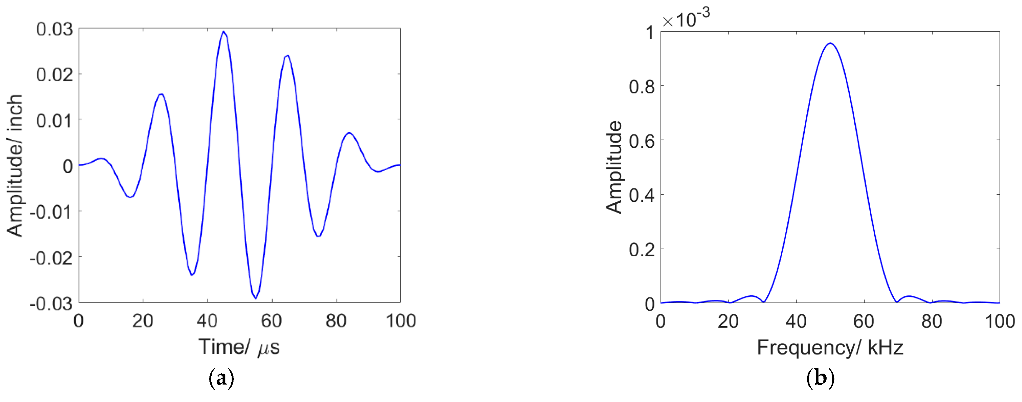
Figure 3.
The excitation signal assumed in the simulation; a) The waveform in the time domain; b) The corresponding wave in the frequency domain.
Figure 3.
The excitation signal assumed in the simulation; a) The waveform in the time domain; b) The corresponding wave in the frequency domain.
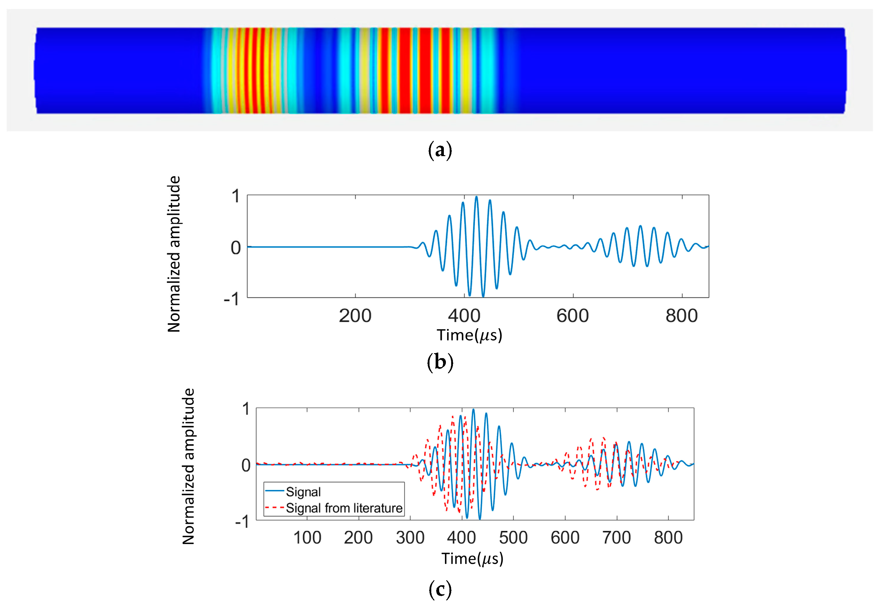
Figure 4.
Comparison of the literature result [
28] and the excitation signal dispersion from the proposed simulation work. (a) Excitation signal dispersion contour from the proposed simulation, (b) Dispersive time domain signal from the proposed simulation, (c) Comparison of the dispersive signals from the literature [
24] and the proposed simulation. (Excitation: (a, b) A five-cycle Hann-windowed 50kHz signal; (c) A ten-cycle Hann-windowed 40kHz signal).
Figure 5.
Illustration of pipe structure type classification: (a) Clamp (~inch); (b) Welding (~inch); (c) Localized Corrosion(~inch); (d) General Corrosion(~feet); (e) Pitting Corrosion (Radius: ~200µm).
Figure 5.
Illustration of pipe structure type classification: (a) Clamp (~inch); (b) Welding (~inch); (c) Localized Corrosion(~inch); (d) General Corrosion(~feet); (e) Pitting Corrosion (Radius: ~200µm).
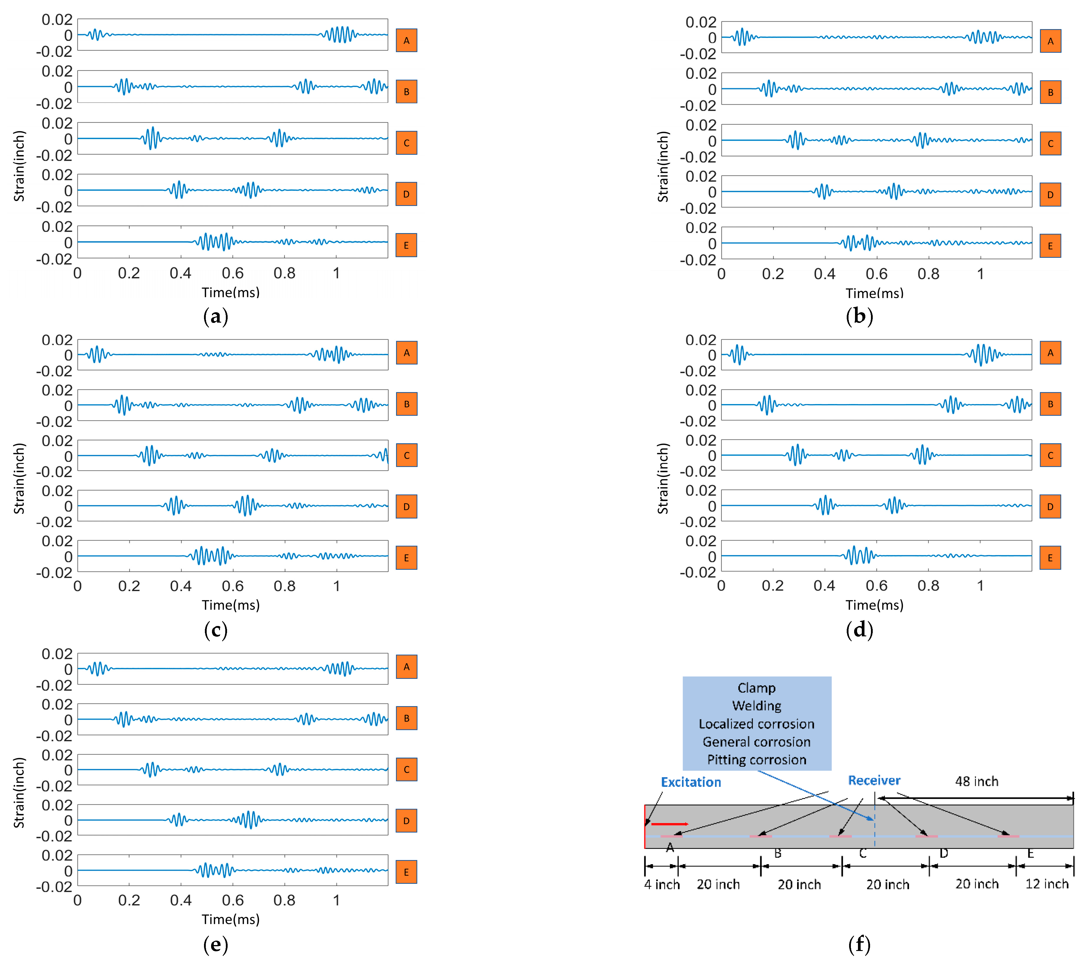
Figure 6.
The time-domain acoustic waveforms from 5 sensors (A-E) by the excitation and the typical reflected signals of the five types of damage: (a) echoes of clamp; (b) echoes of welding; (c) echoes of localized corrosion; (d) echoes of general corrosion; (e) echoes of pitting corrosion; and (f) the schematic diagram of fiber optic acoustic sensors positions for pipeline structure monitoring.
Figure 7.
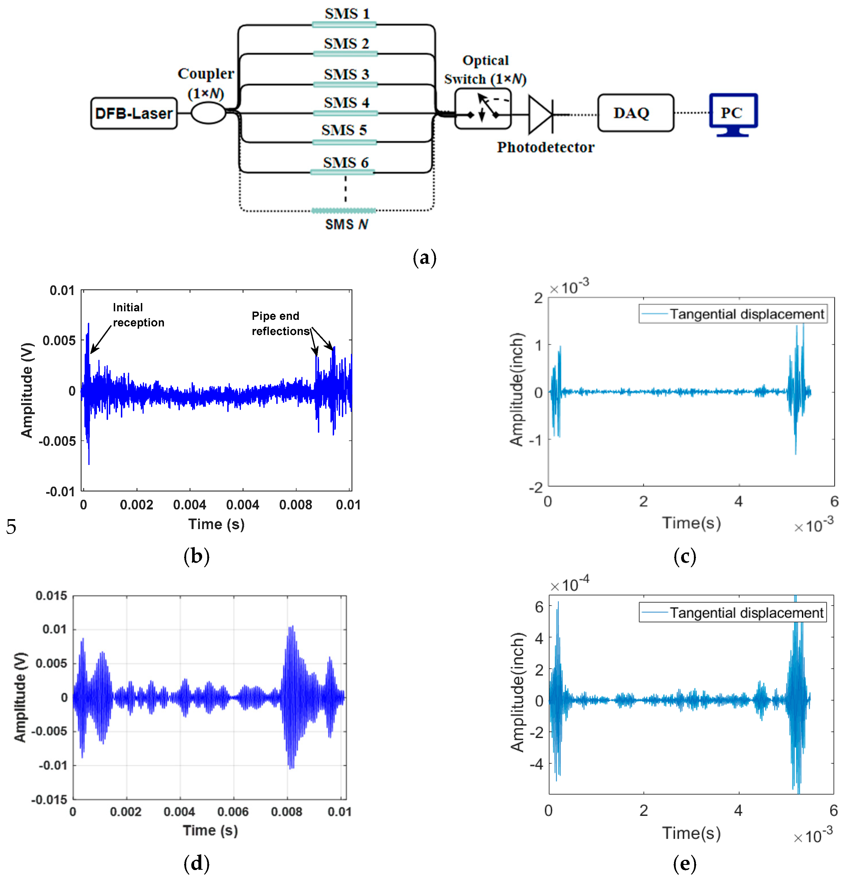
Comparative Analysis of Experimental and Simulated Results for a 32 kHz Quasi-Distributed SMS Fiber Sensor: (a) Multiplexed Interrogator Schematic; (b) Received Signal with 32 kHz Excitation; (c) Simulated 32 kHz, 5-Cycle Sinusoidal Signal for Validation at Same Location as Experiment; (d) Time-Domain Signal after Passband Filtering (26-36 kHz); (e) Filtered Simulated 32 kHz, 5-Cycle Sinusoidal Signal (26-36 kHz).
Figure 8.
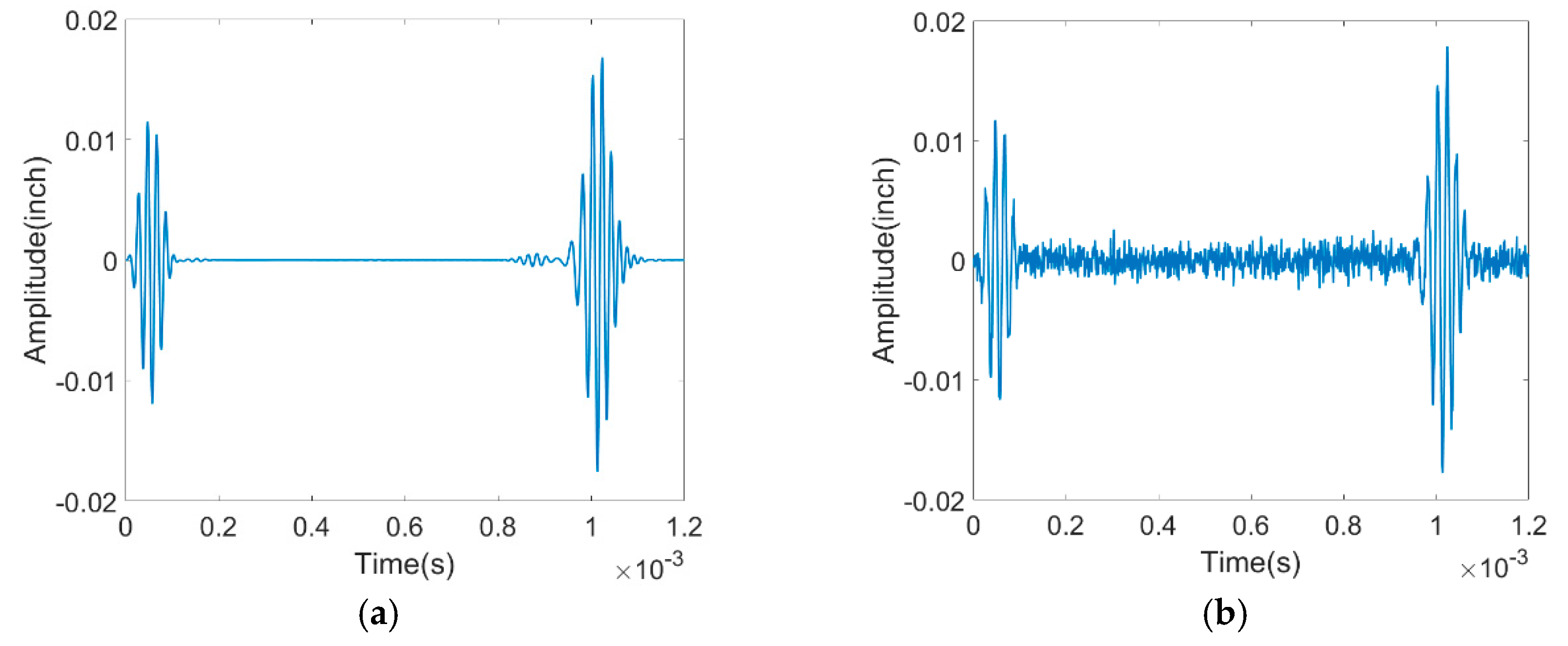
(a) Simulated Pure Signal - Original signal without any noise interference, (b) Signal with 9.63 dB Noise Added - The pure signal is altered by introducing a 9.63 dB noise component to simulate real-world conditions.
Figure 8.
(a) Simulated Pure Signal - Original signal without any noise interference, (b) Signal with 9.63 dB Noise Added - The pure signal is altered by introducing a 9.63 dB noise component to simulate real-world conditions.
Figure 9.
Resulting signal for a healthy pipeline based on distributed sensing system (a) without noise and (b) with Gaussian noise (SNR=9.63dB); and the resulting signal based on quasi-distributed sensing system(12 signal channels) (c) without noise and (d) with Gaussian noise (SNR=9.63dB). The resulting signal is shown as a 2D time-space plot, where the x-axis represents time, and the y-axis represents the length of the pipeline.
Figure 10.
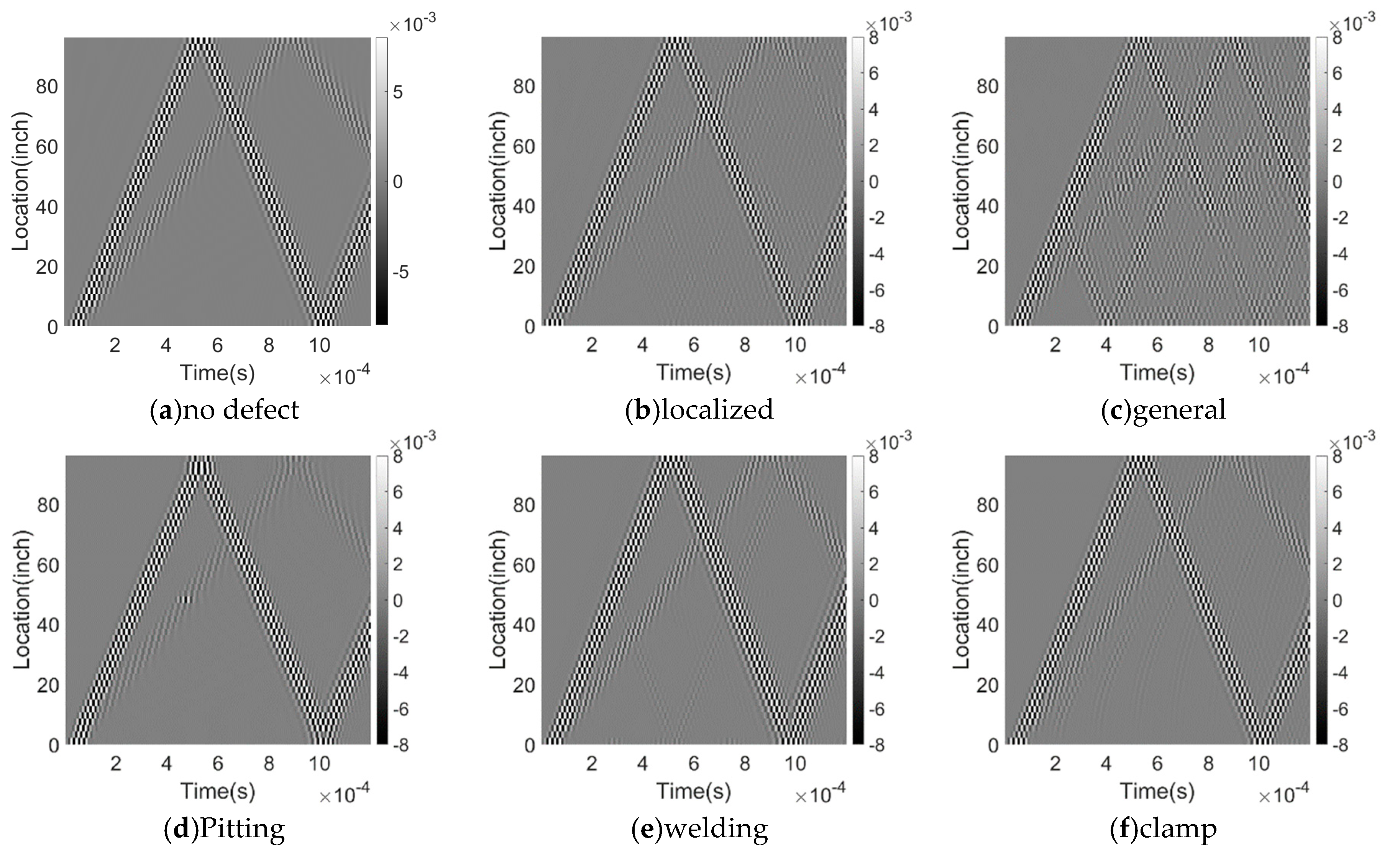
Time-space plots for a pipeline with (a) no defect, (b) localized corrosion, (c) general corrosion, (d) pitting corrosion, (e) welding, and (f) clamp. Each plot shows the resulting signal from a different type of defect or feature. The x-axis represents time, and the y-axis represents the spatial location along the pipeline. The color scale indicates the amplitude of the signal.
Figure 11.
Two-Layer CNN for Signal Classification: Input data is a 2D tensor of size (batch size, 1200, 46). The network consists of two convolutional layers (16 and 32 filters, kernel size of 10), followed by max pooling layers (pool size of 2), two fully connected layers (64 and 6 neurons) for multi-class classification.
Figure 12.
Comparing test accuracy distributions of 6 CNN models with different layer number and activation function for pipeline signal classification.
Figure 12.
Comparing test accuracy distributions of 6 CNN models with different layer number and activation function for pipeline signal classification.
Figure 13.
matrix for pipeline condition classification using (a) fully distributed acoustic sensing (DAS) system and (b) quasi-distributed acoustic sensing (qDAS) system with 12 sensor segments. The confusion matrix shows the number of true positives, true negatives, false positives, and false negatives for each pipeline condition class. The classification accuracy for fully DAS system is 99% and for quasi-DAS system is 96%. The results suggest that the fully DAS system achieved higher classification accuracy compared to the qDAS system, particularly in distinguishing between different types of corrosion.
Figure 14.
Comparison of Confusion Matrices for (a) Fully Distributed and (b) Quasi-Distributed Sensor Systems with Gaussian Noise and SNR=9.63dB.
Figure 14.
Comparison of Confusion Matrices for (a) Fully Distributed and (b) Quasi-Distributed Sensor Systems with Gaussian Noise and SNR=9.63dB.
Figure 15.
The sensor system is configured as a fiber sensor that covers the pipe, with the measurement units evenly distributed along its length.
Figure 15.
The sensor system is configured as a fiber sensor that covers the pipe, with the measurement units evenly distributed along its length.
Figure 16.
The prediction accuracy changes with different sensor numbers under different signal-noise ratio.
Figure 16.
The prediction accuracy changes with different sensor numbers under different signal-noise ratio.
Table 1.
Dimensional parameters of the steel pipeline model.
Table 1.
Dimensional parameters of the steel pipeline model.
|
) |
) |
) |
| 96 |
12 |
0.5 |
Table 2.
Material property parameters of the steel pipeline model.
Table 2.
Material property parameters of the steel pipeline model.
|
) |
) |
) |
) |
| 96 |
7850 |
|
0.32 |
Table 3.
Dimensional parameters of pipeline feature types.
Table 3.
Dimensional parameters of pipeline feature types.
Pipe
feature |
Clamp |
Welding |
Localized
Corrosion |
General
Corrosion |
Pitting |
| Variable |
Axial Length:
(0.02~0.2 inch)
Stiffness factor:
(5e+06~6.5e+06N/m) |
Axial length:
(0.02~0.2 inch)
Depth:
(0.05~0.2 inch) |
Axial length:
(1~8 inch), Depth:
(0.01 ~0.45 inch) |
Axial length:
(0.5~5 feet)
Depth:
(0.05~0.45inch) |
Radius:
(0.5~10 inch)
Depth:
(0.05~0.45 inch) |
Case
number |
20 |
30 |
40 |
40 |
25 |
| Description |
The elastic support loaded by clamps (blue region); |
The discontinuity and material property changes between the pipeline and the welded portion |
A rectangular notch on the inner surface of the pipeline, indicating presence of corrosion in a specific area. |
Evenly reduction in pipeline thickness |
Micrometer-scale localized corrosion of a specific type |
Table 4.
The training and validation accuracy comparison of different optimizers.
Table 4.
The training and validation accuracy comparison of different optimizers.
| CNN_model |
CNN structure |
| Model 1 |
1 Layer + ‘relu’ |
| Model 2 |
1 Layer + ‘sigmoid’ |
| Model 3 |
1 Layer + ‘tanh’ |
| Model 4 |
2 Layer + ‘relu’ |
| Model 5 |
2 Layer + ‘sigmoid’ |
| Model 6 |
2 Layer + ‘tanh’ |
Table 5.
Comparison of Classification Performance Metrics for Fully Distributed and Quasi-Distributed Sensor Systems with Gaussian Noise, SNR = 9.63 db.
Table 5.
Comparison of Classification Performance Metrics for Fully Distributed and Quasi-Distributed Sensor Systems with Gaussian Noise, SNR = 9.63 db.
| |
Fully Distributed |
Quasi-Distributed |
| Classification report |
Precision |
Recall |
Precision |
Recall |
| Welding |
100.00% |
100.00% |
100.00% |
100.00% |
| Localized corrosion |
100.00% |
100.00% |
100.00% |
100.00% |
| General corrosion |
100.00% |
100.00% |
100.00% |
100.00% |
| Pitting corrosion |
100.00% |
96.00% |
95.83% |
92.00% |
| Clamp |
96.15% |
100.00% |
96.00% |
96.00% |
| No defect |
100.00% |
100.00% |
92.31% |
96.00% |
Table 6.
Comparison of Classification Performance Metrics for Fully Distributed and Quasi-Distributed Sensor Systems with Gaussian Noise, SNR = 9.63dB.
Table 6.
Comparison of Classification Performance Metrics for Fully Distributed and Quasi-Distributed Sensor Systems with Gaussian Noise, SNR = 9.63dB.
| |
Fully Distributed |
Quasi-Distributed |
| Classification report |
Precision |
Recall |
Precision |
Recall |
| Welding |
96.15% |
100.00% |
100.00% |
96.00% |
| Localized corrosion |
100.00% |
100.00% |
100.00% |
100.00% |
| General corrosion |
100.00% |
96.00% |
96.15% |
100.00% |
| Pitting corrosion |
96.00% |
96.00% |
90.00% |
90.00% |
| Clamp |
95.74% |
90.00% |
96.00% |
96.00% |
| No defect |
90.57% |
96.00% |
90.00% |
90.00% |
