Preprint

Article

Combining low-cost SLAM and SfM-MVS for Rural and Forest Road-side Slope Erosion Control: a methodology

Altmetrics

Downloads

180

Views

Comments

Christopher Gomez^*,Muhammad Anggri Setiawan,

Noviyanti Listyaningrum,

Balázs Bradák,

Yousefi Saleh

Christopher Gomez^*,Muhammad Anggri Setiawan,

Noviyanti Listyaningrum,

Balázs Bradák,

Yousefi Saleh

This version is not peer-reviewed

Submitted:

26 April 2023

Posted:

27 April 2023

You are already at the latest version

Alerts

Abstract

Hillslope and mountain roads are often the source of erosion, which in turn can lead to larger landslides and other types of mass-movements. For this reason, low-cost repeat surveys that can be done by practitioners and not solely scientists and engineers is essential. To solve this issue the present contribution shows the testing and applicability of a mix of SfM-MVS and low-cost SLAM technology to provide erosion information. The low-cost SLAM generated between 300 ~ 900 points per square meter, while SfM-MVS created between ~11,000 to 900,000 points. The density is however a trade-off against a spatially varying error, although the variability at the road-cut scale only ranges from 2 cm vertically to 2.5 cm in x,y,z based on the C2C algorithm. Furthermore, this error tends to be more important in the higher section of the cutout (further away from the sensor and at a flatter angle). It is thus possible to measure small-scale roadside change, providing that the change is in the range of >5 cm (adding the maximum potential error twice) and providing that the road-cut is such that the sensors can be brought close to the surface (camera or sensor on a pole). The authors suggest that it can be a solution for state and agencies with limited funding and that cannot afford regular laser or for roadside that are difficult to access.

Keywords:

Subject: Environmental and Earth Sciences - Soil Science

1. Introduction

In recent years, road-side erosion and road-deformation measurement and monitoring has greatly benefited from the development of LiDAR technology, especially when mounted on vehicles on the roads and on rails. However, these vehicles and associated-set-up are best adapted for highways and roads, which offer good height and width clearances. Forestry roads and mountain roads are thus out of reach for those technologies, and although LiDAR has become a widespread technology [1], it has only occurred in a handful of countries, and traditional airborne LiDAR still has difficulties to penetrate the dense canopy to offer sufficient ground information [1]. Thus forested road-side erosion remains a challenge to measure in most regions of the world. In the present contribution, we thus present a low-cost methodology (one needs an iPad® and a regular digital camera and a regular computer), to monitor road-side outcrop and erosion features, which can also be used to monitor mountain trails erosion [2].

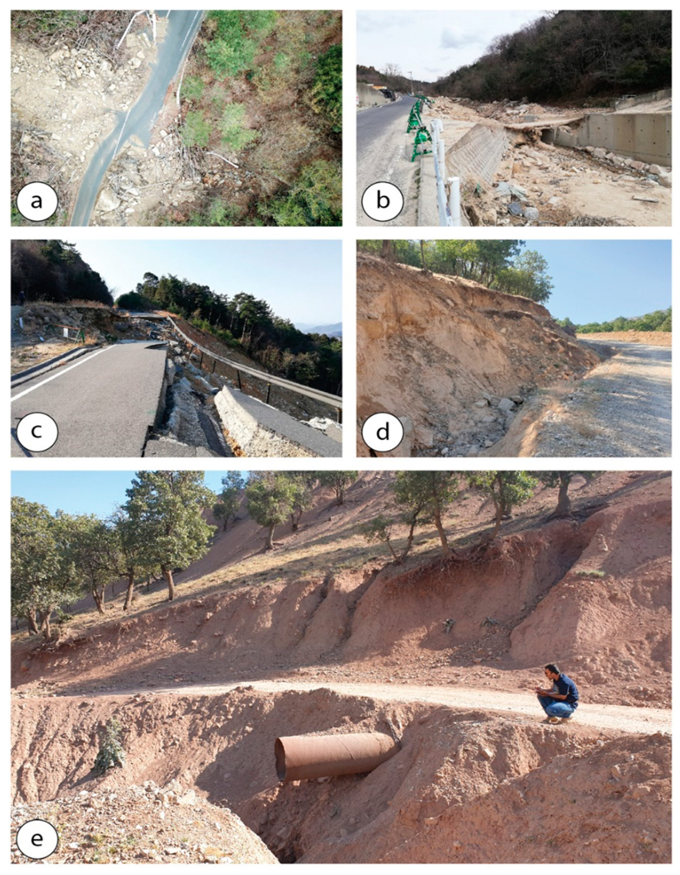
Road-side erosion materializes in different ways over the pathway, it can either be debris-spreading from the slope onto the road, making it unfit for purpose for a while (e.g. when a debris-flow crosses a road – Figure 1-a), or it can be a road failure due to short-lived high-impacts erosional events from waterways (e.g. Figure 1-b) or in the vicinity of mass movements (e.g. Figure 1-c). Road-side erosion also occurs as a progressive process, with measured changes of a few to a few tens of millimeters per year along hillroads of Spain for instance [3]. This erosion being accentuated when vegetation cover is sparse (e.g. in Iran Figure 1, d and e), eventually leading to land degradation [4].

The road itself also plays a crucial role in erosion and sediment transport, and it has become part of watershed restoration practices to let mountain and forest roads go in state of disrepair or even remove them, in order to limit erosion [5,6]. Comparing revegetated and decommissioned roads to newly reopened forestry mountain roads, interrill erodibility coefficient has been measured to vary between 0.007 and 0.2 x10⁶ kg s m^-4 for undisturbed forest floor to 1.0 and 1.8 x10⁶ kg s m^-4 for reopened road (cf. [7] for the erodibility coefficient equations) [7]. This work shows that the road plays an important role as it opens the canopy and the understory, but the position on the slope as well as the length of the slope are also essential controls in mountainous areas [8]. In wetter environment, concentrated erosion can be more severe, and even with existing understorey. In the Zenjiagou watershed (China), the average erosion is 18.61 t ha^-1 and annual precipitation 592 mm [9]. Their analysis emphasizes the role of multiple factors in controlling unpaved road erosion, the road gradients, where the erosion amount (EA) in ton per ha is correlated with the road gradient (Rg) as EA = 1695.2Rg-4008.7 (R² = 0.6) for cropland and EA = 1583.3Rg-6493.9 (R² = 0.5) for forest and grassland areas. The Erosion amount is further correlated with the drainage size per unit of road (Ur) with EA = 57.583Ur-533.87 (R² = 0.78) [9]. There is thus a combination of road characteristics, position, maintenance and management as well as land-cover and environmental factors that all combine in a complex way, so that field survey is essential.

To measure the 3D morphology of a surface and to detect any change over time, a high-resolution topographic model with a constrained error is necessary, to avoid mis-interpreting error for change of the surface over time. Pointcloud dataset generated from TLS have notably proven to provide accurate repeats over time [10], one can either rely on sequences of photographs [11], where most of the time the SIFT (Scale Invariant Feature Transform) algorithm [12] or one of its derivatives is used to match the different features images [1], and error is determined thanks to the RANSAC (RANdom Sample And Consensus) algorithm [13]. These two algorithms have been key to the development of the SfM-MVS method (Structure from motion and Multiple View Stereophotogrammetry), allowing the automation of feature matching and of the photogrammetric process [14]. Such method has been demonstrated to construct accurate models of gullies and rills of a few tens of centimeter scales, with a relative accuracy at check points to be between 87.7% and 97.5%. For linear scale-values, the same authors even rich values of 99.1% [11]. These results echo other findings, stating that SfM-MVS is generating results comparable to those of TLS (Terrestrial Laser Scanner) [14]. In a gully headcut-erosion study from 5 different locations, the comparison of SfM-MVS and TLS provided a RMSE (Root Mean Square Error) between 0.025 m and 0.091 m with a bias of 0.003 m and 0.019 m [15], which also confirms the previous conclusions. Recent research, has emphasized the importance to have clearly defined tie-points and GCPs (Ground Control Points), either obtained from a GNSS-RTK (Global Navigation Satellite System), or GNSS-PPK (Global Navigation Satellite System, post-processing Kinematic), or from TLS or topographic total stations, to scale the SfM-MVS model, and also detect any smoothing of the topographic details. It has been further suggested that even the high-contrast of the target could help the model locally, but also provide an error assessment that is overly optimistic [16].

In the present contribution, the authors aimed to propose a low-cost and light-weight system, that is highly portable and thus can be carried by practitioners and scientists on steep roads, and forested mountain trails. The feasibility of this objective is tested with a reflectorless and targetless method to compensate the issue related with targets [16].

2. Materials and Methods

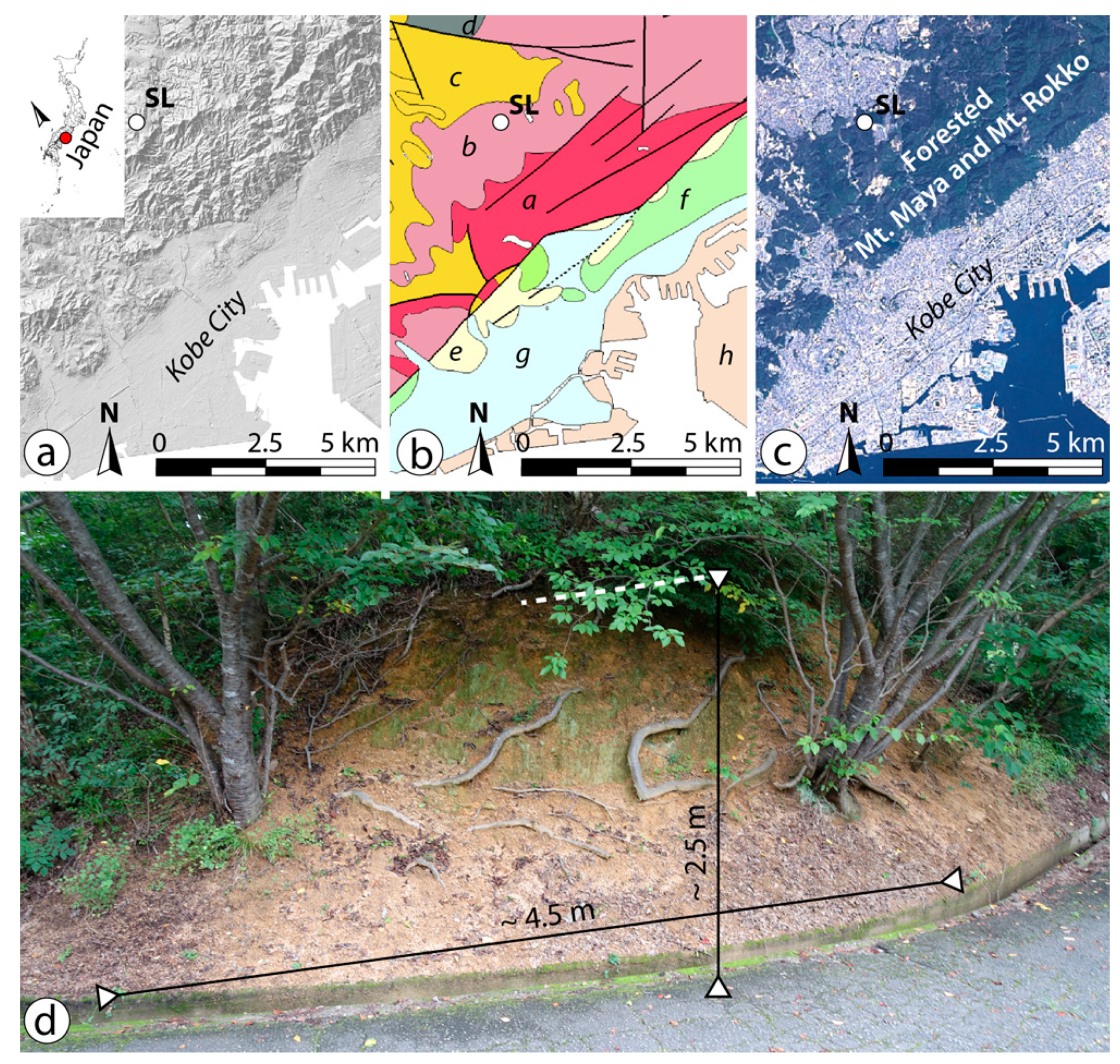
The fieldwork was conducted along a closed mountain road-side under forest cover in the mountains located above Kobe City in Japan (Figure 2). The road is mostly used for recreational activities, although it is maintained to service the telecommunication tower it connects to. The outcrop, which serves as research material, is about 4.5 m long and 2.5 m high. It is cut into weathered graniodiorite material from which a sandy soil has developed. At the survey site, it is laced with tree roots (Figure 2-d).

The research was conducted in the field in July 2022, and SLAM (Simultaneous Localization and Mapping) laser scanning and photographic survey. The SLAM laser scanning was conducted with an ipad Pro, using the inner laser-sensor and the open-source application RTAB-Map (Real-Time Appearance-Based Mapping) developed by a French research team in photogrammetry and robotic for 3D mapping [17,18] and available on github. The photographic survey is composed of 178 photographs taken at the site for SfM-MVS purposes, with a handheld Sony RX100 III Cybershot camera, which is mounted with a Zeiss Vario-Sonnar lense. The position of the camera was varied horizontally from the road plane, as well as vertically, by raising the camera over one’s head (about 2 m) and at chest level and a few tens of centimeter from the ground. The angle between each shot was < 30 degrees and the photographs were taken in a row, so that there is an overlap between each photograph, following the commonly suggested methodology for SfM-MVS [1].

Proceeding after field data acquisition, the SLAM-LiDAR dataset was converted from the binary file to asci file for reading in Cloud-Compare®. The photographs were processed using the software Metashape-Pro commercialized by Agisoft, following the now accepted process of (1) sparse point generation, (2) point-cloud densification [1], but the pointcloud was not scaled nor oriented at this stage (as it is usually done with UAV and other data that include geometric information at acquisition). The pointcloud from SfM-MVS was then processed in CloudCompare, by scaling and orienting the point-cloud using 4 common points found on both pointclouds. It resulted in a RMSE (Root Mean Square Error) of 0.019 m at the four points used to overlap the two pointclouds (Another method would have been to use targets, but it is suspected to create over-optimistic results [16]), and two pointclouds that are the base of the present analysis (Table 1).

The data analysis was then conducted as follows, using the two point-clouds in the python environment using the “Pandas dataframe” data analysis add-on as well as the sklearn computer learning toolbox:

(1) the two surfaces were compared using the C2C (Cloud to Cloud algorithm in CloudCompare), in order to define areas of local error (based on the concept that the two methods being different in what data are being collected and how the 3D is being produced, there is no intrinsic reason for the error to vary similarly).

(2) As the present research is to test a method that can be done from the road-side, the two point-clouds were acquired from the edge of the road (without stepping on the slope), and as there is slant on the slope. As the distance from the camera and the laser increases with the height, the first assumption is that the error may overall increase with height.

(3) As surface reflectance for the laser, and the photography may be hampered in very dark areas, areas that are not visible from the road, the correlation between the error was tested against the RGB value (the 0 value being black and the combination of the highest values (3x255) being white).

(4) Then a further assumption was made: vegetation, especially if it moves with the wind may be a source of error. Therefore, the Green band was tested against the local error.

(5) Finally, in order to test for any characteristic and pattern in the dataset that may exist besides the three assumptions above, the data were exported as text-file to the python environment, and using the Pandas dataframe, variable pairing and comparison was also performed.

3. Results

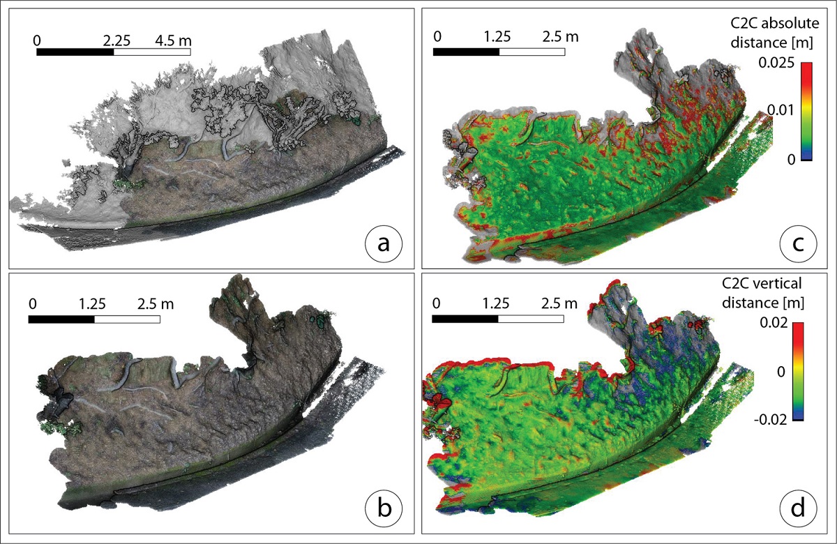
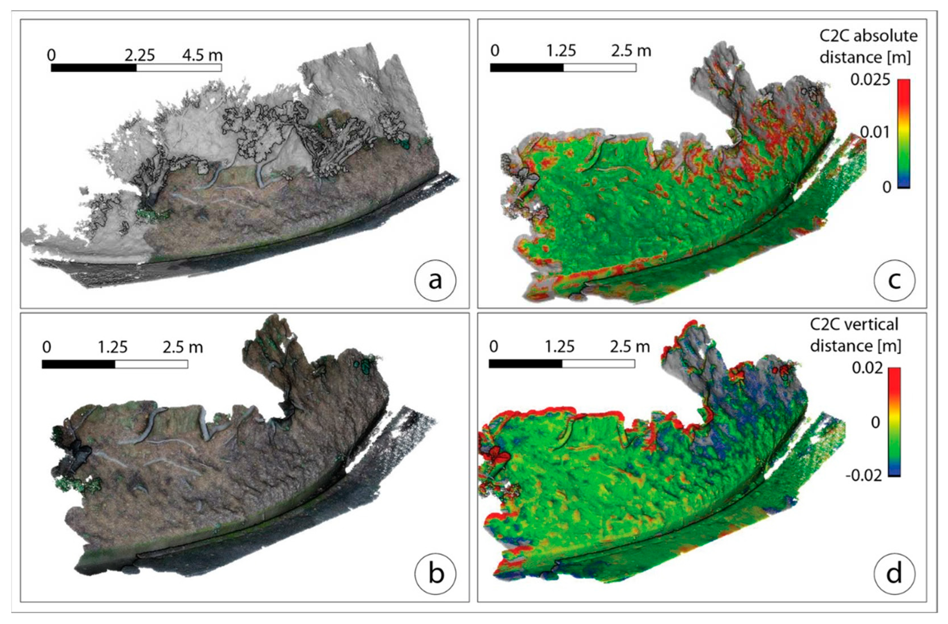
The section of the two pointclouds that overlap were extracted (Figure 3-a) and the area with the two pointclouds (Figure 3-b) have shown an absolute distance comprised between 0 and 0.025 m using the C2C absolute distance estimation algorithm. The central part of the studied outcrop is below 0.005 m absolute distance, with increased at and above 0.025 m at the top-edge of the pointclouds, as well as at the road-side water-drain, which has vertical walls. At the lower extent, the top corner-edge of the wall is also displaying errors in excess of 0.025 m (Figure 3-c). Within the central part of the outcrops, there are also some thin lineaments of discrepancy between the two pointclouds, and those have emerged on the top and back part of the tree-roots that are visible at the surface. Considering the distance in the vertical direction, a similar pattern of errors on the edges at the top of the outcrop was also calculated, but not in the lower part where the drain is and less significantly where the roots are located. This signifies that the error in the water drain is on the horizontal axis, and so are a large number of the errors where the tree roots are located (Figure 3-d).

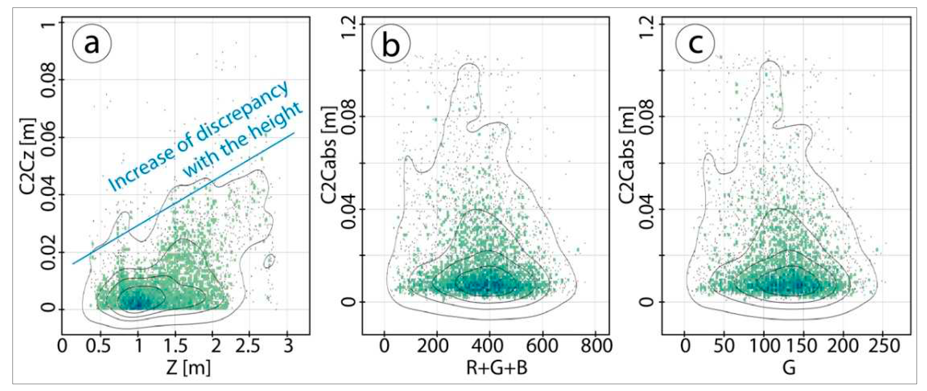
One of the assumption of the error distribution is that the distance to the camera or the laser optic was a source of error, and comparing the elevation above the road in meter (Z) with the results of the C2C algorithm of vertical data (C2Cz), the visual trend seen in Figure 3-d is confirmed from the scatter-plot (Figure 4). Although the error envelopes show a crude increase of C2Cz with Z, the density shows a dual-peak pattern with a broad spread of error underneath 1 m and then another broad spread above 1 m. The other assumptions were that vegetation on the outcrop may influence the results as well as any dark spot, but the distribution of the discrepancy between the two pointclouds as expressed by the results of the C2C absolute distance (C2Cabs) shows that the spread of error is only linked to the density of the dataset (figure 4), in other words, the more data are collected the higher the chances to have outliers and errors. There is thus no relation between the darkness of the scene nor live vegetation at the location, on the day the data was acquired (one will note that weather condition may modify those values).

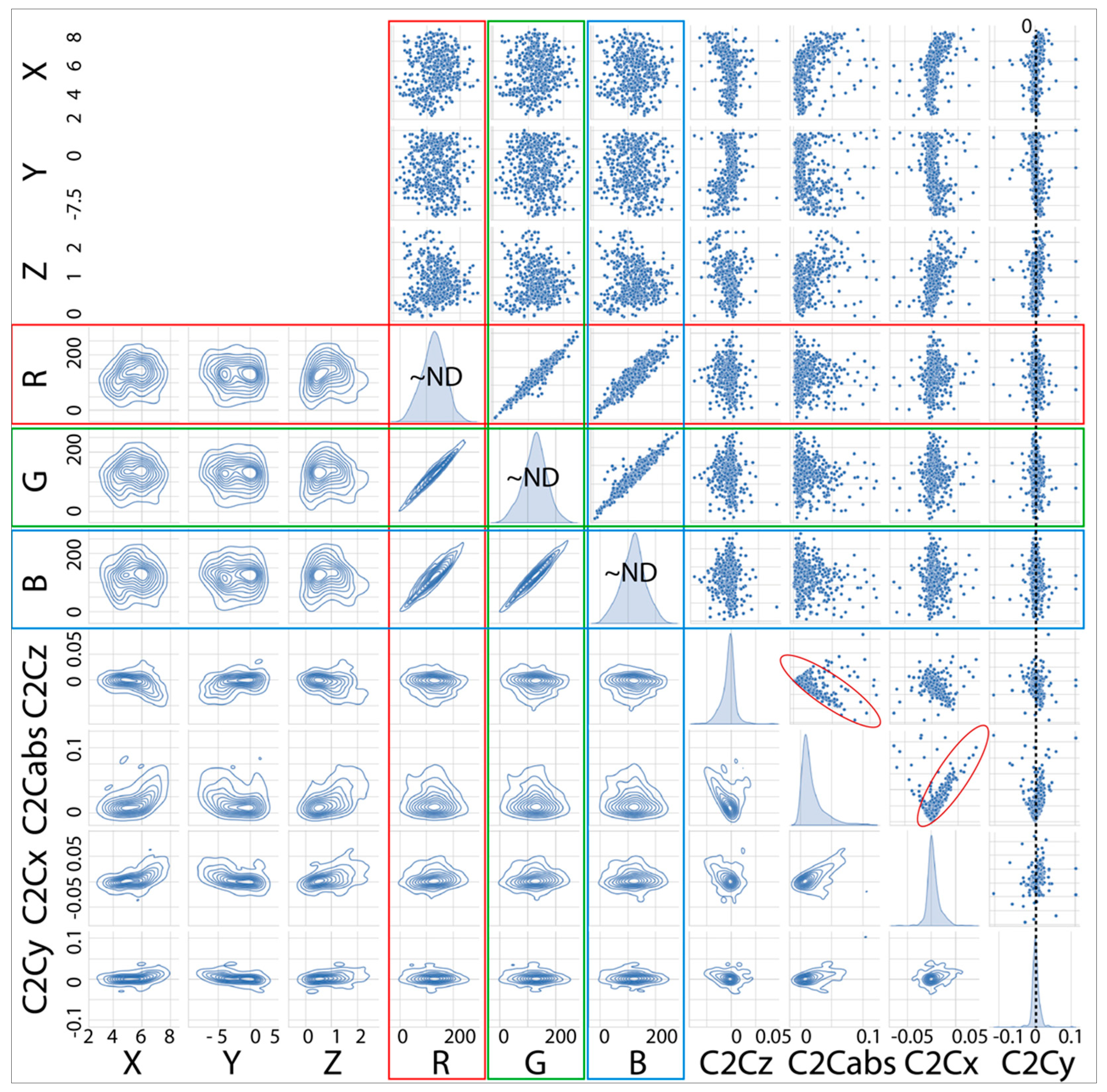
The distribution of colors over the overall survey area is well-spread, creating distribution that are close to normal distribution (ND in Figure 5), meaning that the outcrop is not dominated by dark nor very bright spot. This results in the dataset on a 45 degrees line between the different R,G and B (Figure 5). The error of the different elements of the C2C are also centered on 0, regardless of the spread of the other variables, except for the relationships between C2Cabs and C2Cz and between C2Cabs and C2Cx. For C2Cz, the data are represented in both the negative and positive direction. The difference between the SfM-MVS and the laser data is thus increasing both in the positive and the negative direction vertically. In other word, the Root Mean Square Error would underestimate the error by half. The error in the x direction is showing the same spread in both directions, although the majority of the data shows error in x increasing as the absolute error increases. The other error data are centered and do not show any particular trend however.

4. Discussion

Comparing the pointcloud data produced by SfM-MVS and by SLAM Lidar, the results show a local difference that is up to 2.5 cm absolute distance from the C2C algorithm, and that actually spreads vertically and in the X direction by a similar value. The absolute value of spread of 2.5 cm actually hides a variability that is < 5 cm overall. Therefore, the distribution of error is essential to better use the dataset. Both the camera and the iPad were carried up and down and left and right, so that the distance to the outcrop is supposedly controlled by the slope angle only, and the result have shown that the error increased with the height or more probably with the distance. The problem is that it is not possible to know whether it is an issue generated by the iPad or by the SfM-MVS. Either way, the model generated from the combination of the two methods provide a numerical estimate of the error.

This estimate, however, is only the error intrinsic to one surface, and one needs to use a combination for the two surfaces as it has been shown for the DoD (DEM of Difference) method [19]:

δ u_{D o D} = \sqrt{{({δ z}_{n e w})}^{2} + {({δ z}_{o l d})}^{2}}

In this equation the error propagation (

δ u_{D o D}

) is calculated as the combination of the error in Z in both surfaces, here written as the old and the new. A similar approach can be adopted - not for a DEM - but for the surfaces using the absolute error of each pointcloud, so that it can be resampled based on the necessity, so that:

\sum_{i = 1}^{n} \sum_{j = 1}^{m} [{C 2 C a b s}_{(i)} + {C 2 C a b s}_{(j)}] < E s t i m a t e d e r o s i o n

where, the C2Cabs for all the points of the first pointcloud i=1 to n, and the points on the second pointcloud are j from 1 to m, and these absolute values are similar to the results of

δ u_{D o D}

. When comparing two pointclouds, you can then determine whether the measure is reliable by comparing the “Estimated erosion” to the error, and then sample only the data that are of interest. For this purpose, one can export a file with the information included in the structure, like in the dataset that is provided with this contribution:

Pts n, X,Y,Z, […],R,G,B,C2Cabs₁, C2Cz₁, C2Cx₁, C2Cy₁, C2Cz₁, […], C2Cabs₂, C2Cz₂, C2Cx₂, C2Cy₂, C2Cz₂ , where the subscript 1 and 2 are the same data produced in the present study, but expanded to one (and potentially more) surfaces.

Based on the present research result, the combination of iPad and SfM-MVS works well for erosion that is > 5 ~ 10 cm between two time-steps, but forestry experiments on the forest road erosion [3] is certainly not appropriate for the present method, unless deep rills develop on the tracks [2]. Erosion on the roadside in Iran as seen in the photographs of the road in Iran are more appropriate.

5. Conclusions

The present contribution shows that with only an iPad and a regular camera, with at least one pointcloud generated by each method, and arguably better with several repeat of each method, it is possible to approximate the local error and then repeat the same operation at different times to create differential surfaces to measure erosion. Moreover, the error is not constrained to a small set of targets, nor is it impacted by the addition of targets. The combination of these two low-costs method allows geomorphologic and erosion surveys even in hard-to reach, even for practitioners and academics without sufficient access to buy the still expensive surveying tools.

Author Contributions

The present research is the result of an international collaborative project between Indonesia, Iran and Japan. All the authors have contributed to the manuscript and reflection on the project. The first author first drafted the paper, and then it was reworked and improved by the co-authors.

Funding

The present research was partly supported by the international collaboration funding of Kobe University, Graduate School of Maritime Sciences.

Data Availability Statement

The data are available on demand.

Acknowledgments

In this section, you can acknowledge any support given which is not covered by the author contribution or funding sections. This may include administrative and technical support, or donations in kind (e.g., materials used for experiments).

Conflicts of Interest

The authors declare no conflict of interest.

References

Gomez, C. Point-cloud Technology for Geomorphologists; Springer: Germany, 2022; pp. 1–245. [Google Scholar]
Salesa, D.; Cerda, A. Soil erosion on mountain trails as a consequence of recreational activities. A comprehensive review of the scientific literature. J Environ Manage 2020, 271, 110990. [Google Scholar] [CrossRef] [PubMed]
Arnaez, J.; Larrea, V. Erosion Processes and Rates of Road-Sides of Hill-Roads (Iberian System, La Rioja, Spain). Phys. Chem. Earth 1995, 20, 395–401. [Google Scholar] [CrossRef]
Panagos, P.; Borrelli, P.; Robinson, D. FAO calls for actions to reduce global soil erosion. Mitig Adapt Strateg Glob Chang 2020, 25, 789–790. [Google Scholar] [CrossRef]
Switalski, T.A.; Bissonette, J.A.; DeLuca, T.H.; Luce, C.H.; Madej, M.A. Benefits and impacts of road removal. Front Ecol Environ 2004, 2, 1195–1207. [Google Scholar] [CrossRef]
Yousefi, S.; Moradi, H.; Boll, J.; Schonbrodt-Stitt, S. Effects of road construction on soil degradation and nutrient transport in Caspian Hyrcanian mixed forests. Geoderma 2016, 284, 103–112. [Google Scholar] [CrossRef]
Foltz, R.B.; Copeland, N.S.; Elliot, W.J. Reopening abandoned forest roads in northern Idaho, USA: Quantification of runoff, sediment concentration, infiltration and iterrill. J Environ Manage 2009, 90, 2542–2550. [Google Scholar] [CrossRef] [PubMed]
Xu, X.-L.; Liu, W.; Kong, Y.-P.; Zhang, K.-. L, Yu, B.; Chen, J.-D. Runoff and water erosion on road side-slopes: Effects of rainfall characteristics and slope length. Transp Res D Transp Environ 2009, 14, 497–501. [Google Scholar] [CrossRef]
Wang, C.; Liu, B.; Yang, Q.; Pang, G.; Long, Y.; Wang, L.; Cruse, R.M.; Dang, W.; Wang, E. Unpaved road erosion after heavy storms in mountain areas of northern China. Int Soil Water Conserv Res 2022, 10, 29–37. [Google Scholar] [CrossRef]
Gao, C.; Li, P.; Hu, J.; Yan, L.; Latifi, H.; Yao, W.; Hao, M.; Gao, J.; Dang, T.; Zhang, S. development of gully erosion processes: A 3D investigation based on field scouring experiments and laser scanning. Rem Sens Env 2021, 265, 112683. [Google Scholar] [CrossRef]
Yao, Y.; Li, J.; Duan, P.; Cheng, F. Research on three-dimensional model reconstruction of slope erosion based on sequence images. Opt Laser Technol 2019, 110, 209–218. [Google Scholar] [CrossRef]
David, G.L. Distinctive image features from scale-invariant keypoints. Int J Comput Vis 2004, 60, 91–110. [Google Scholar]
Satkin, S.; Rashid, M.; Lin, J. 3dnn: 3d nearest neighbor. Int J Comput Vis 2015, 111, 69–97. [Google Scholar] [CrossRef]
James, M.R.; Robson, S. Straightforward reconstruction of 3D surfaces and topography with a camera: Accuracy and geoscience application. J Geophys Res 2012, 117, 1–17. [Google Scholar] [CrossRef]
Gomez-Gutierrez, A.; Schnabel, S.; Berenguer-Sempere, F.; Lavado-Contador, F.; Rubio-Delgado, J. Using 3D photo-reconstruction methods to estimate gully headcut erosion. Catena 2014, 120, 91–101. [Google Scholar] [CrossRef]
Schwendel, A.C.; Milan, D.J. Terrestrial structure-from-motion: Spatial error analysis of roughness and morphology. Geomorphology 2020, 350, 106883. [Google Scholar] [CrossRef]
Labbe, M.; Michaud, F. Multi-Session Visual SLAM for Illumination-Invriant Relocalization in Indoor Environments. Frontiers Robotic AI 2022, 9, 1–14. [Google Scholar] [CrossRef] [PubMed]
Labbe, M.; Michaud, F. RTAB-Map as an Open-Source Lidar and Visual SLAM Library for Large-Scale and Long-Term Online Operation. J Field Robotic 2019, 36, 416–446. [Google Scholar] [CrossRef]
Brasington, J.; Langham, J.; Rumsby, B. Methodological sensitivity of morphometric estimates of coarse fluvial sediment transport. Geomorphology 2003, 53, 299–316. [Google Scholar] [CrossRef]

Figure 1. Road-side erosion from sudden and progressive events (a) Debris-flow apron in the mountain between Hiroshima City and Kure City in Japan after the 2018 heavy-rain event; (b) waterway erosion in near Kure City in Japan; (c) road collapse at the head-scarp of a landslide; (d and e) progressive road-side erosion and storm-water pipe erosion in Iran.

Figure 2. Field research location and characteristics. (a) Grey-scaled relief map of Kobe and the mountains at the back, SL indicates the survey site seen in the photograph “d”; (b) Simplified geological map where the black lines are the known faults and the dotted black line, the supposed ones. On the map the letters in italic symbolize the different geological formations as follows: a: massive graniodiorite from Mesozoic Late Cretaceous; b: massive granite from Mesozoic late cretaceous; c: non-marine sandstone from Cenozoic; d: mixed rocks from Early Jurassic; e: Cenozoic Quaternary sediment mixtures; f: Quaternary terrace deposit; g: Holocene valley floor, river and coastal deposits; h: Holocene reclaimed land (source of the data: Geological Survey of Japan). (c) Satellite imagery of Kobe City, where the forested mountains adjacent to the city emphasizes its recreational and managed aspects, so that erosion control is an essential element (source of the data: Geographical Authority of Japan); (d) photograph taken in July 2022 of the surveyed road-side wall.

Figure 3. This is a figure. Schemes follow the same formatting.

Figure 4. Test of the assumptions that may increase the discrepancy between the two pointclouds: the height (Z) from the ground and distance to the recording apparatus, the brightness or darkness of the location (R+G+B) and finally the presence of green (G), which may move with the wind.

Figure 5. Pairing diagram of a random subsample (5,000 points) showing the density of points (with 10 equal bins (10x500 points), the probability distribution of the sample as well as the sample pointclouds themselves. X,Y,Z represents the Cartesian coordinates of the scene, R,G,B are the three color-channels attached to each point, C2Cz is the vertical difference (as it would appear in a DoD – DEM of differences), C2Cabs is the closest absolute distance between points and C2Cx and C2Cy are the distances calculated in the X and Y direction. In the top left corner of the matrix, the meaningless comparisons with the different XYZ were omitted (all the metric values are in meters).

Table 1. Basic characteristics of the two pointclouds generated by SLAM-LiDAR and SfM-MVS.

Point-cloud	Number of pts	Nb of pts in 10 cm radius	Density (per m²)
SLAM-LiDAR	364,054	1 – 890	315 – 30,617
SfM-MVS	17,704,702	3 -19870	11,548 – 900,735

Disclaimer/Publisher’s Note: The statements, opinions and data contained in all publications are solely those of the individual author(s) and contributor(s) and not of MDPI and/or the editor(s). MDPI and/or the editor(s) disclaim responsibility for any injury to people or property resulting from any ideas, methods, instructions or products referred to in the content.

© 2023 by the authors. Licensee MDPI, Basel, Switzerland. This article is an open access article distributed under the terms and conditions of the Creative Commons Attribution (CC BY) license (http://creativecommons.org/licenses/by/4.0/).

Copyright: This open access article is published under a Creative Commons CC BY 4.0 license, which permit the free download, distribution, and reuse, provided that the author and preprint are cited in any reuse.