Preprint
Article

A Visual Enhancement Network with Feature Fusion for Image Aesthetic Assessment

Altmetrics

Downloads

114

Views

23

Comments

0

A peer-reviewed article of this preprint also exists.

This version is not peer-reviewed

Submitted:

27 April 2023

Posted:

28 April 2023

You are already at the latest version

Alerts
Abstract
Abstract: Image aesthetic assessment (IAA) with neural attention has made significant progress due to its effectiveness in object recognition. Current studies have shown that the features learned by convolutional neural networks (CNN) at different learning stages indicate meaningful information. The shallow feature contains the low-level information of images and the deep feature perceives the image semantics and themes. Inspired by this, we propose a visual enhancement network with feature fusion (FF-VEN). It consists of two sub-modules, the visual enhancement module (VE module) and the shallow and deep feature fusion module (SDFF module). The former uses an adaptive filter in the spatial domain to simulate human eyes according to the region of interest (ROI) extracted by neural feedback. The latter not only takes out the shallow feature and the deep feature by transverse connection, but also uses a feature fusion unit (FFU) to fuse the pooled features together with the aim of information contribution maximization. Experiments on standard AVA dataset and Photo.net dataset show the effectiveness of FF-VEN.
Keywords: 
Subject: Computer Science and Mathematics  -   Computer Vision and Graphics

1. Introduction

With the increasing application of digital images, the studies of image aesthetic assessment (IAA) have made significant development. IAA has favorable commercial application value and potential. Feature extraction has long been a question of great interest in IAA [1]. Early studies focused on photographic methods and human perception. Deng et al. [2] summarized the manual production features and the deep features, indicating the limitations of machine learning. Among the early efforts, the diversity of aesthetic features and the complexity of photographic methods resulted in the poor performance of the models with manual extraction.
Recently, deep learning has become a hot topic for IAA [3], which overcomes the limitation of hand-crafted feature extraction. Neural networks have shown good advantages for image analysis and processing [4,5,6]. Dai et al. [7] introduced the existing research in the field of intelligent media. The pooling layers was utilized to increase the speed of processing the low-level features [8]. Talebi et al. [9] modified the last layer of convolutional neural networks (CNN), directly predicting the aesthetic score distribution. It transforms the classification model into a distributed task, increasing the training speed and improving the performance of neural networks. Based on [9], In [10], VGGNet stacks the convolutional layers, pushing the network depth to more than 16 weight layers. [11] showed that intermediate convolution layers of CNN contain meaningful information about the complexity of images. Thus, we analyze the network structure and try to fuse the features of CNN, aiming to combine the low-level information and the abstract image semantics.
Neural attention is a major area of interest within the field of IAA. How to assess the digital images based on human visual characteristics is challenging for researchers. The deep model (TDM) was designed to perceive the image scenes with the advantages of peripheral vision and central vision [12]. Ma et al. [13] introduced A-Lamp that can learn the detailed and overall information of images. The details of images are retained via dynamically selecting image blocks. The overall information is extracted from the attribute graphs of the image blocks. Zhang et al. [14] combined the spatial layout and the details of images on the basis of top-down neural feedback. Inspired by TDM [12], they also proposed GLFN-Net [15]. It calculates the image blocks of region of interest (ROI) and simulates the fovea vision. However, human observation of images is flexible, not in the fixed shape of a rectangle. We attempt to dynamically process the digital images according to ROI.
In this paper, we propose a visual enhancement network with feature fusion (FF-VEN). It is divided into two sub-modules: the visual enhancement module (VE module) and the shallow and deep feature fusion module (SDFF module). VE module simulates the human eyes based on the fovea visual characteristics. It adaptively filters the images according to ROI obtained by neural feedback. SDFF module consists of feature extraction and feature fusion. The shallow feature and the deep feature are taken out by the method of transverse connection. We design a feature fusion unit (FFU) that performs the weighted fusion to maximize the contribution to information. The aesthetic score distribution is learned by minimizing squared earth mover's distance (EMD) loss. Further, FF-VEN is evaluated in the classification task and the regression task. Therefore, the contributions made by this paper are as follows:
1)
We propose an end-to-end training network, consisting of two sub-modules. The former module considers top-down neural attention and fovea visual characteristics. The latter module extracts and integrates the features learned by CNN at different stages.
2)
An adaptive filter is designed to select the filters in the spatial domain. Specifically, each pixel in the images adjusts the parameters of filters according to the normalized interest matrix extracted by neural feedback.
3)
We optimize a feature fusion unit to combine the low-level information and the image semantics. The added pooling layers deal with the corresponding features, increasing the training speed and improving the precision of the predicted score prediction. Besides, it fuses the features for contribution maximization.
The rest of the article is structured as follows. Section 2 introduces the relevant work briefly and Section 3 describes the proposed FF-VEN. Section 4 evaluates the performance of the network and compares it with other models. In Section 5, we summarize the paper.

2. Related Work

There are two basic approaches currently being adopted in research into IAA. One is extracting the image features manually and the other is based on deep learning. On the one hand, hand-crafted feature extraction means designing the aesthetic attributes of digital images on the computer based on photography, psychology, aesthetics, and other subjects. Datta et al. [16] defined the aesthetic image features, including color, structure, and image content, aiming to explore the relationship between human emotions and the low-level features. Reference [17] depended on the global saliency map of images and located the region of visual attention. From a photographer's point of view, Dhar et al. [18] analyzed image layout, sky lighting, and other image attributes. The relative foreground position and visual weight ratio are combined to enhance the visual image features [19]. Tang et al. [20] integrated the regional and global features according to the eye-catching areas. They used a support vector machine (SVM) model for the classification task. However, the methods of hand-crafted feature extraction are unsuitable for all images. It enters a bottleneck, because aesthetics is abstract and the photographic methods are diverse.
On the other hand, deep learning has significant advantages for IAA [2]. For multi-scale image processing, Szegedy et al. [21] proposed GoogLeNet, increasing the width of the network via sparse connections. Because of its great performance on ImageNet, they developed InceptionNet, using optimization algorithms to improve the performance of the model [7]. DMA-NET [22] performed random image clipping and extracted local fine-grained information. A-Lamp learned the detailed information and the overall attributes of the input images [13]. Based on GoogLeNet [21], Jin et al. [23] considered the local and global views of images. They proposed ILG-NET, combing the InceptionNet and the connected layer. Yan et al. [24] obtained the aesthetic image features, including semantics, texture, and color. They weighted points of interest (POI) and segmented the image pixels. They proposed a circular attention network, which ignores irrelevant information and focuses on the attention region when extracting visual features [25]. From the gray value, contrast and spatial position relationships of pixels in color channels, the shallow feature perceives the image attributes like light, tone, clarity, and composition. The semantic information contains image object, theme, context, etc.
At present, the multi-channel frameworks have been widely used for IAA. She et al. [26] captured the image layout, using a special neural network composed of two sub-networks. A pooling layer of the multimodal factorized bilinear (MFB) was used to combine the features [25]. Based on [26], the GIF module integrated the weight generator into the feature fusion part [15]. They down-sampled the images to simulate peripheral vision, which missed the details and failed to assess the high-variance images. A gating unit (GU) performs dynamic weighted combination [27]. GU adds two fully connected layers and a Tanh layer, improving the effectiveness of the networks. It calculates the contribution of features to the result via analyzing the statistical characteristics. Inspired by this, we propose FFU, adding pooling layers for corresponding features based on GU. Ma et al. [13] showed that the ROI captured the spatial layout information of images and calculated the attention area of CNN. Zhang et al. [14] simulated fovea vision by generating image blocks via top-down neural feedback. Similarly, we use the incentive support method [28] to extract the interest matrix of images. However, the area of visual interest is not as the shape of a rectangle when humans assessing images. We develop an adaptive filter, which is such a pixel-based approach that it captures the fine-grained details of an image in any shape.
Early studies treated IAA as a task of aesthetic classification [13,29]. According to the aesthetic score distribution, the average of scores is compared with the threshold value, aiming to divide the images into the high quality images and the low quality images. The aesthetic score distribution is ordered in IAA. Cross-entropy loss in the classification ignores the relationships between scores. The regression model was utilized to assess images [2]. For ordered classes, Zhang et al. [30] showed that the models with the classification task can outperform the regression networks. Due to the cultural background, the emotion states, the physiological condition, and other factors of the assessors, the aesthetic scores are highly subjective. At present, the research mainly focuses on the direct prediction of the aesthetic score distribution. Cumulative distribution function with Jensen-Shannon divergence (CJS) loss was proposed to boost the performance of models [31]. Talebi et al. [8] regarded the score distribution as an ordered class. They used squared EMD loss to predict the score distribution. In this paper, we minimize EMD loss to make the results more accurate.

3. Proposed Method

Figure 1 shows the overall framework of FF-VEN proposed in this paper. VE module uses the excitation support method to extract ROI from images, aiming to get top-down neural attention of ResNet50. Based on ROI, the adaptive filter selects either Laplace filter or Gaussian filter. It also adjusts the parameters of filters depending on the degree of visual interest. SDFF module dynamically fuses the shallow feature and the deep feature of VGG16 [10] taken out via transverse connection. In FFU, the pooling layers are used for the corresponding features. FFU calculates the weights of contribution to information by analyzing the statistical characteristics of the features. Next, the pooled features are dotted with their contribution weights, and then put into fusion. Finally, EMD loss is selected to predict the score distribution.

3.1. Top-down Neural Attention

In this paper, ROI represents the level of interest of all pixels in the form of a two-dimensional matrix. The interest degree is calculated via top-down neural feedback from the decisive pixels to the all pixels of the original image. For the computer, the interest matrix shows the region with the prominent feature that CNN pays attention to when predicting. For humans, the value of the interest matrix represents the degree of attraction to the pixel by human eyes. On the basis of the probabilistic winner-take-all (WTA) model, the incentive support method [28] can calculate the interest matrix with the same size as the input image. In statistical concepts, the marginal winning probability P o i represents the attention rate transmitted from the decisive pixels, i.e.,
P o i = j = 1 N P o i o j
where o i is a pixel of the overall pixel set in the input image, N is the number of the decisive pixels in the upper layer generated by o i . In (1), P ( o i ) sums the pixel’s effect degree after quantization between the two layers. In the excitation backprop algorithm, neurons transmit signals through the excitation propagation. The marginal winning probability P o i is obtained via the top-down connections based on the conditional winning probability P ( o i o j ) . If the excitation connection m i , j exists, P ( o i o j ) is defined as:
P o i o j = m i , j o ^ i c j
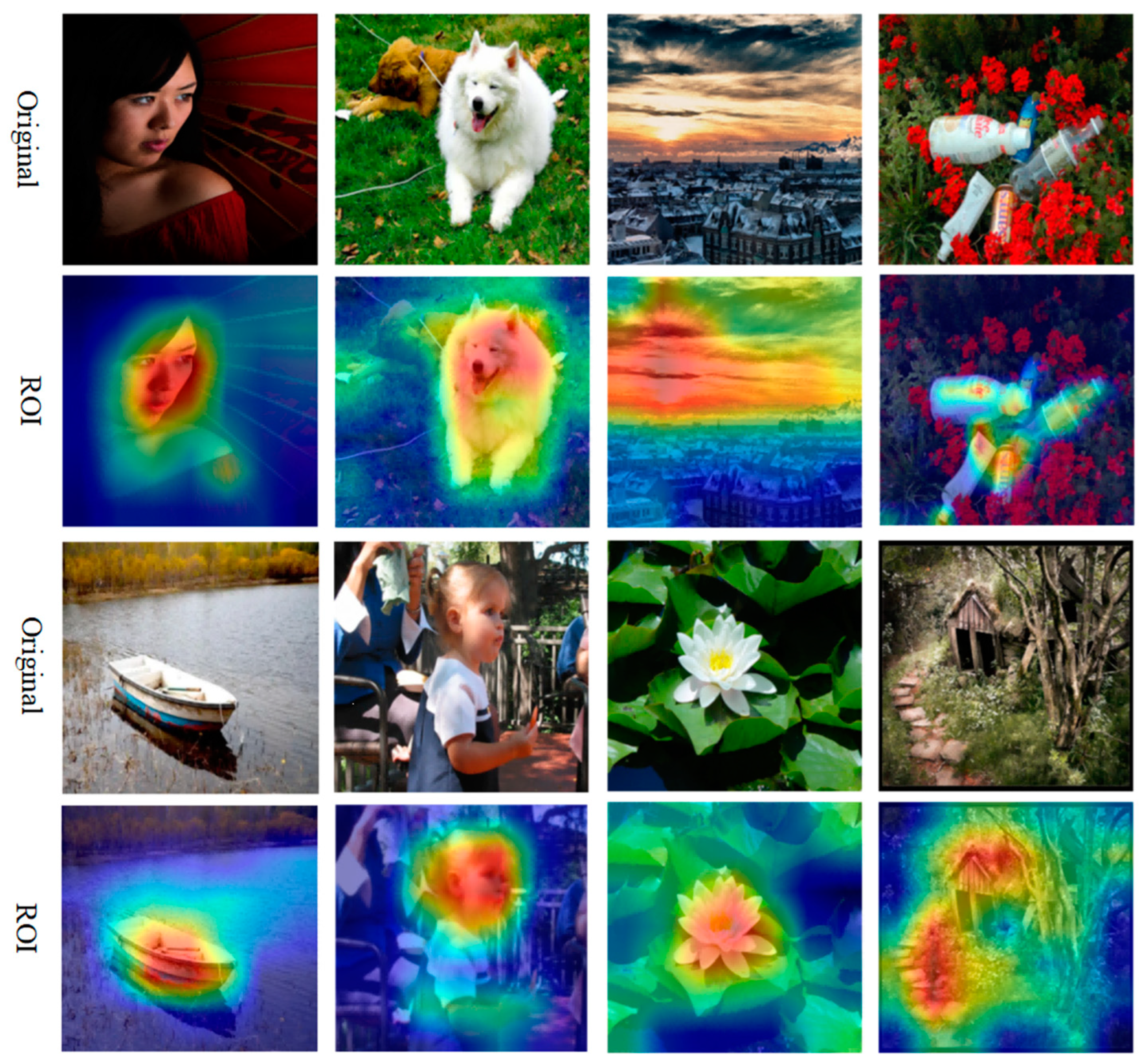
where m i , j represents the connection weight between o i and o j , o i means the response of o i , and c j is the normalization factor. According to (1) and (2), the recursive propagation of top-down signals can calculate the interest matrix of images layer by layer. The interest matrix represents ROI in pixels when CNN makes decisions. In this paper, pre-trained ResNet50 is used to extract the interest matrix. Some examples are shown in Figure 2. ROI of images is highlighted by the pseudo-color technique. In Figure 2, ROI not only distinguishes between the foreground and the background, but also displays the degree of neural attention.

3.2. Adaptive Filtering

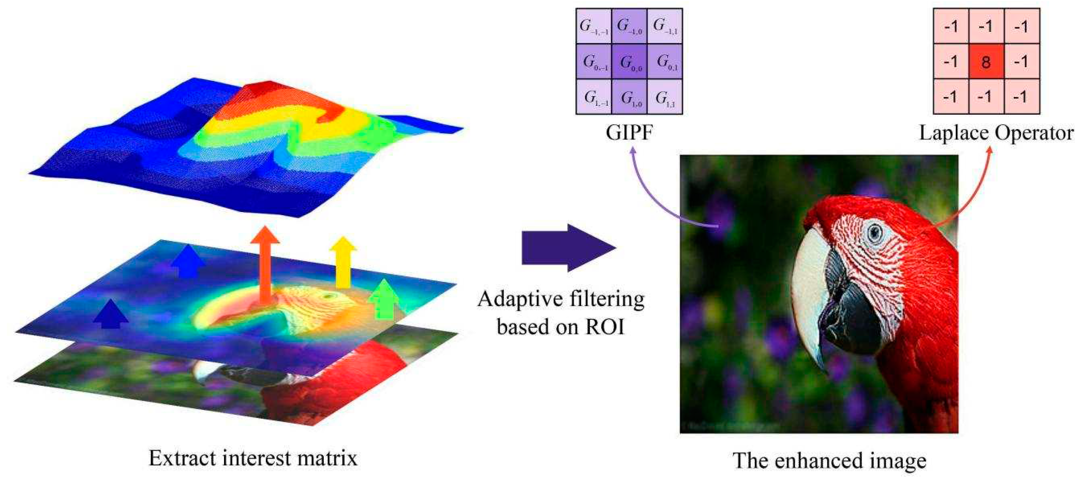
An adaptive filter is designed to simulate human eyes based on the fovea visual characteristics. The spatial domain filters conform to the convolution process of CNN, so the adaptive filter uses Laplace filter and Gaussian filter. The outermost edge of the images is retained to keep the image size unchanged. As shown in Figure 3, adaptive filtering is carried out on the basis of the interest matrix extracted in Section 3.1. First, the interest matrix is processed by the min-max normalization method. The value of the threshold is set as the average of the interest matrix. Experiments show that the average value accounts for about 60% of the maximum value. Next, the interest degree of each pixel is compared to the value of the threshold, selecting to sharpen or to blur.
On the one hand, for the process of sharpening, the Laplace operator is used to calculate the details of the images. The Laplace operator of 4 neighborhood pixels is defined as:
g L 4 ( x , y ) = f ( x , y 1 ) + f ( x , y + 1 ) + f ( x 1 , y ) + f ( x + 1 , y ) 4 f ( x , y )
where f ( x , y ) is the pixel located at coordinates ( x , y ) . There is another kind of expression of Laplace operator. Its definition is shown below:
g L 8 ( x , y ) = i = 1 1 j = 1 1 f ( x + i , y + j ) 9 f ( x , y )
where g L 8 ( x , y ) means the Laplace operator with diagonal distribution. g L 8 ( x , y ) detects more details and texture, combining fine-grained attributes of 8 neighborhood pixels. In addition, irregular noise belongs to fine-grained information in the spatial domain. Due to the noise’s impact on image assessment, the high-pass filter processes images directly. The high-boost filtering combines the original images and the weighted results of Laplace filtering. It linearly enhances the texture and the details of images, i.e.,
g ( x , y , k , b ) = f ( x , y ) + k g L ( x , y ) + b
where g L ( x , y ) represents the pixel after Laplace filtering and f ( x , y ) means a pixel of the input images. b and k are coefficients of the high-boost filtering and their values depend on the degree of the neural attention. In (5), the high-boost filtering adds the fine-grained texture (obtained by the Laplace operator) to the original pixel. The greater interest degree causes the greater enhancement of texture and details. On the other hand, two-dimensional Gaussian low-pass filter (GIPF) is utilized for the blurring process:
G ( x , y , σ ) = 1 2 π σ 2 e ( x 2 + y 2 ) 2 σ 2
where x and y are the coordinates of pixels, σ is the standard deviation of GIPF and its value is determined by the interest matrix. According to (6), the smaller the value of σ , the severer the peak’s change in Gaussian function, and the lower the blurring degree. On the contrary, the larger value of σ results in the higher blurring degree. Table 1 shows the specific parameters of the filters. Max is the highest interest degree of the input image and threshold is set to choose the corresponding filter.
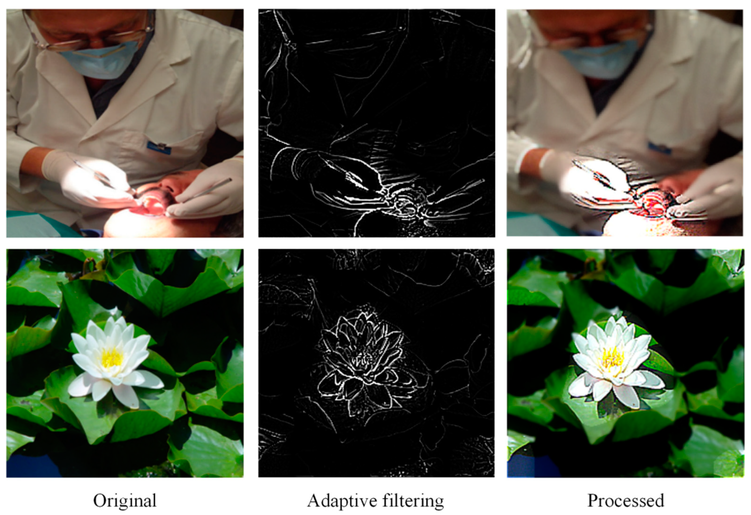
As mentioned above, the adaptive filter in the spatial domain with contrast processing achieves the goal of visual enhancement. Figure 4 shows some examples of this step. Column 2 shows the quadrupling of the results. In Figure 4, the adaptive filter sharpens or blurs the images in different degrees based on ROI. The process of sharpening leads to the brighter foreground and the sharper details. The result of blurring is weakening the presence of the background. For computer vision, the adaptive filter increases the difference between pixels of different interest levels based on the feedback after identifying the object. The cooperation of neural attention in Section 3.1 and the adaptive filtering in Scetion 3.2 takes advantage of the underlying physiological responses that human consciousness drives behavior.

3.3. Features at Different Stages

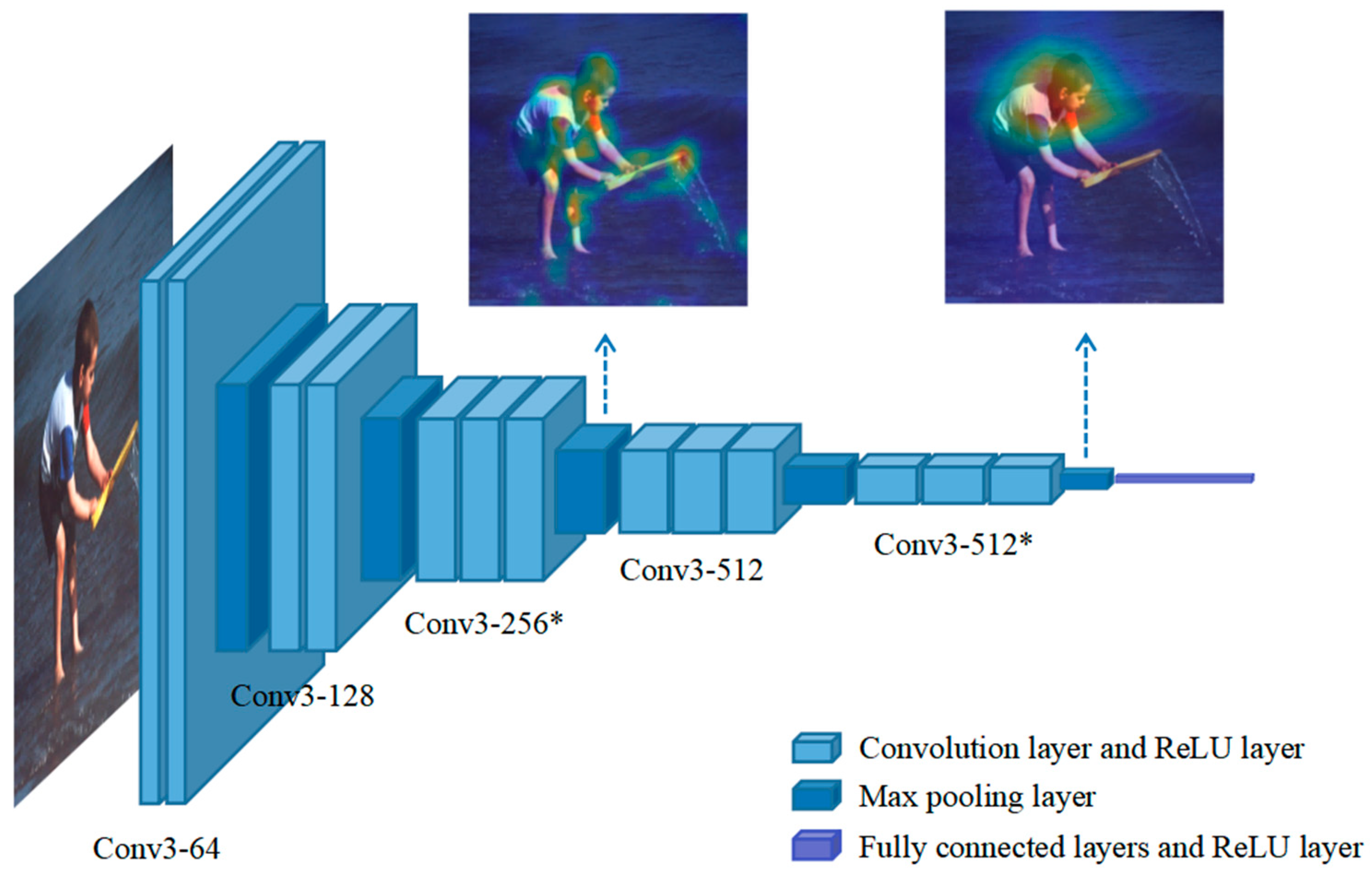
Current studies have found that there are different meanings of features learned by CNN at different learning stages [11]. The shallow feature contains the low-level information of images, such as color, edge, and texture. The deep feature perceives abstract semantic information. Similar to InceptionNet [7], SDFF module broadens the network structure, aiming to improve the performance of models. We use VGG16 [10] as the baseline and take out the shallow feature and the deep feature from different convolution layers. Figure 5 shows an example of the results. The main parameters of VGG16 are listed in Table 2. The max pooling layer after each convolution layer is omitted. From the Conv3-256* layer, we take out the shallow feature, whose size is 28 × 28 × 256 after passing through the max pooling layer. The deep feature is taken from the Conv3-512* layer. Its size is 7 × 7 × 512 . The above process is mathematically expressed as:
I 1 = P l 1 ψ W 1 I 0 I 2 = P l 2 ψ W 2 I 1
where I 0 represents an input image, I 1 and I 2 are the output of the transverse connection, ψ W i I i 1 is the state function of VGG16, and P l i I i 1 is the feature pooling function with i = 0 , 1 , 2 . In (7), I 1 is taken out when VGG16 is the state function ψ W 1 I 0 . By the feature pooling function P l 1 I 1 , the shallow feature I 1 is obtained. Similarly, the deep feature I 2 is taken out by the method of transverse connection. Adding the shallow feature reduces the influence of the deep feature on the results. In this way, the low-level and semantic information of the images can be integrated to improve the network performance.

3.4. Feature Fusion Unit

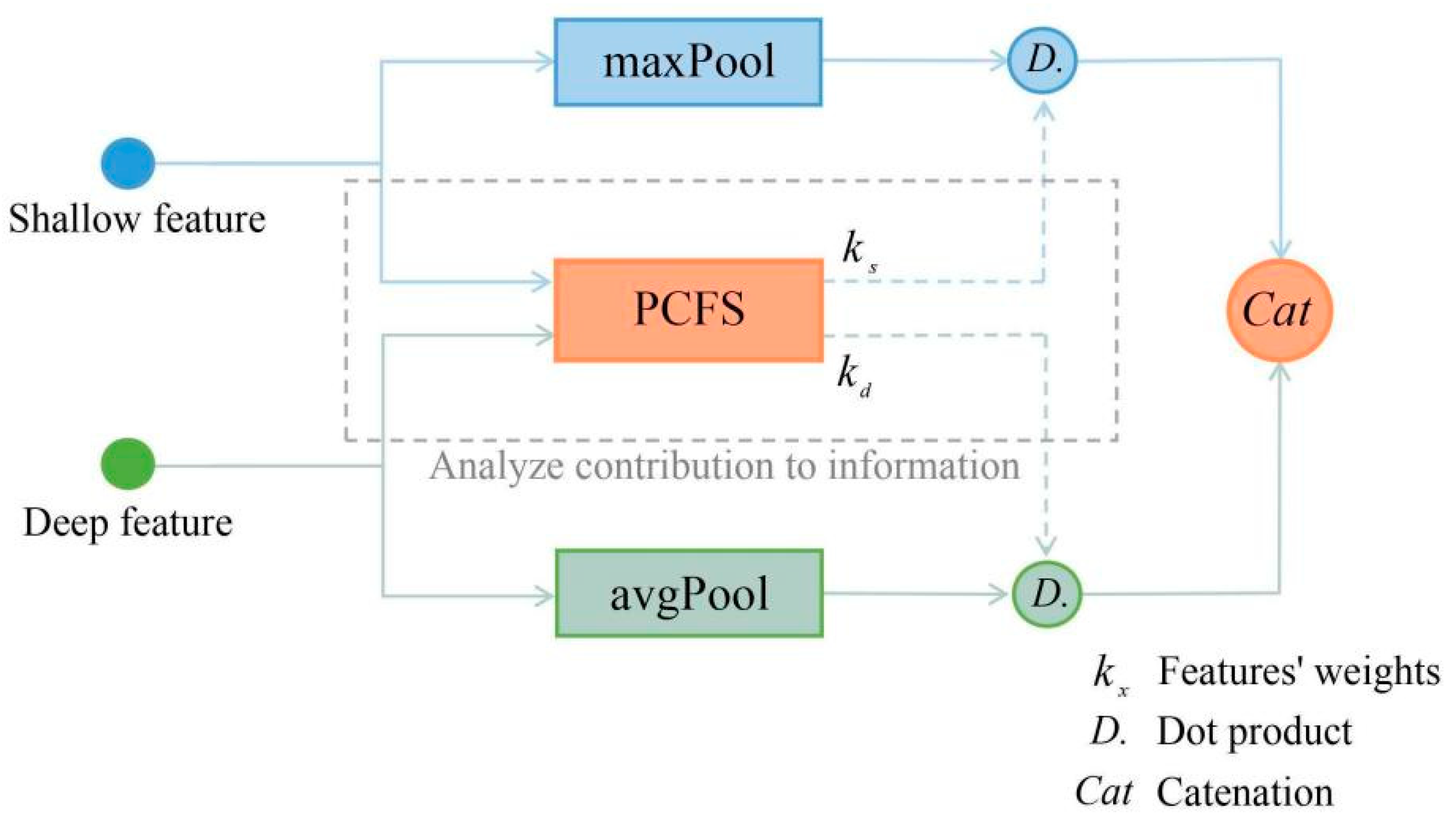
After taking out the features, SDFF module needs a feature fusion mechanism to combine the shallow feature and the deep feature. Figure 6 shows FFU after fine-tuning. PCFS means a pooling layer, a catenation layer, a fully connected layer, and a Sigmoid layer in turn. The pooling layer analyzes the statistical characteristics of the features. The next layers calculate the weights (denoted by k x with x = s or d in Figure 6) of the pooled features. s means the shallow feature and d is the deep feature. k x represents the contribution weight of the feature to the information. Then, the shallow feature and the deep feature pass through the max pooling layer and the average pooling layer, respectively. Max pooling not only selects the data with higher recognition but also provides the nonlinearity factor for FFU. The deep feature is the results that CNN learns in the later stage, so it influences CNN greatly. Average pooling considers all of the deep information. Because the sizes of the two pooling layers are 7 × 7 , the shallow feature and the deep feature are rescaled to 7 × 7 × 256 and 7 × 7 × 512 . Afterwards, we take the dot product of each pooled feature and its k x . Finally, the results are fused by the catenation layer. The main parameters of FFU are showed in Table 3.

3.5. EMD Loss

In AVA dataset and Photo.net dataset, the score distribution is intrinsically ordered. For ordered classes, the performance of classification models is better than regression frameworks. However, the classification task ignores the relationships between classes of score distribution. EMD loss penalizes mis-classifications according to class distances. In this paper, EMD loss is minimized to predict the score distribution directly. Because of the impact of the number of assessors on credibility, the distribution is normalized. The definition of EMD loss is shown below:
E M D l , p = 1 N i = 1 N C D F l i C D F p i r 1 r
where C D F x ( i ) represents the cumulative distribution function as n = 1 i e d n ( 1 i N ) . d n means the nth normalized number of assessors. x = l , p . (l is the label distribution and p is the predicted distribution.) In (8), EMD is the minimum distance between the mass of two score distributions. We set r as 2 to punish the Euclidean distance between CDFs, aiming to optimize the network.

4. Experiments

In this section, the performance of FF-VEN is evaluated on AVA dataset and Photo.net dataset. Compared with previous studies, FF-VEN is a promising model for IAA.

4.1. Datasets

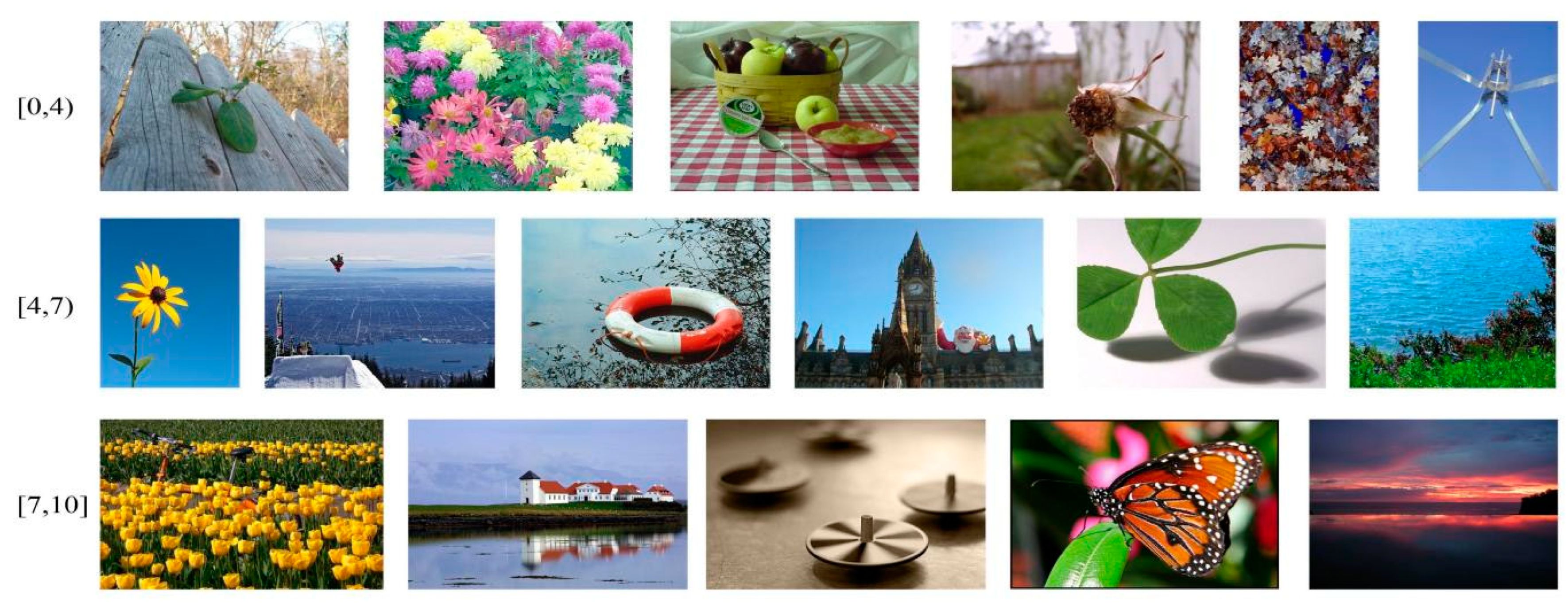
AVA dataset [32]: AVA dataset is a popular dataset for IAA because of the large number of images, the diversity of content, and the consistency of data. It can be seen at http://www.dpchallenge.com/. For an image, there are 66 semantic labels, 14 style labels, and a label distribution with 10 scores (from 1 to 10). In AVA dataset, the higher scores mean the higher quality. For an image with the average score in a certain interval, its score distribution tends to be Gamma or Gaussian [32]. Figure 8 shows some examples of AVA dataset. On average, each image is assessed by about 200 people, including professional image workers, photographers, and photography enthusiasts. AVA dataset contains more than 250,000 images. We remove the images whose variance is high or whose average score is 5. Thus, 235,086 images are used for training, 18,987 for verification, and 1,000 for testing.
Figure 7. The examples of images with the average score in different intervals in AVA dataset. Line 1, the images with the average score in [0,4); Line 2, the images with the average score in [4,7); Line3, the images with the average score in [7,10].
Preprints 72050 g007
Photo.net dataset [33]: Photo.net dataset contains about 20,000 images. We collect them from https://www.photo.net/, a platform for photography enthusiasts to share images. This website offers discussion forums, image reviews, galleries, etc. People assess images based on aesthetics and creativity, with a score between 1 and 7 for each. Photo.net explains that 1 means low quality and 7 means high quality. Reasons for a high score include rich colors, interesting composition, and eye-catching content. In Photo.net dataset, the images are diverse, which is a challenge for deep learning. Excluding invalid images and lost images, 16,663 images are obtained by crawlers. 14,000 images are used for training, 1,000 for verification, and the remaining 1,663 images are used for testing.

4.2. Details of the Experiment

The size of the input images is 224 × 224 × 3 . The images are resampled by the ANTIALIAS algorithm of PIL package in PYTHON library. Batch size is 16, initial learning rate is 1e-3, momentum is 0.9, learning decay rate is 0.0002, and epoch is 10. The number of iterations of AVA dataset is 14,693 and that of Photo.net dataset is 1,042. Our network is based on the open source TorhchRay, Caffe, and PyTorch frameworks. We use a single NVIDIA GeForce GTX 1650 GPU.
Based on the direct prediction of the score distribution, we evaluate FF-VEN in the classification task and the regression task. In the regression task, we use these indicators: Pearson linear correlation coefficient (LCC), Spearman rank-order correlation coefficient (SRCC), mean absolute error (MAE), and root mean square error (RMSE). The evaluation index formulas are showed as:
L C C = 1 N 1 i = 1 N l i l ¯ σ l p i p ¯ σ p S R C C = i = 1 N l i l ¯ p i p ¯ i = 1 N l i l ¯ 2 i = 1 N p i p ¯ 2 M A E = i = 1 N | p i l i | N R M S E = i = 1 N p i l i 2 N
where l is the label distribution and p is the predicted distribution, l ¯ is the average of l, σ l is the standard deviation of l, p ¯ is the average of p, σ p is the standard deviation of p. LCC applies to normally distributed data to predict the accuracy of the model. SRCC is suitable for nonlinear data. It calculates the correlation of the scores in the corresponding position in arrays between the prediction distribution and the label distribution. The values of SRCC and LCC vary between 0 and 1. The larger value means the better model performance. RMSE measures the deviation between the predicted results and the labels. MAE calculates the average of residuals directly. MAE and RMSE are expected to be smaller. In the classification task, we calculate Mean of the score distribution and compare it with the value of the threshold. We define Mean as:
M e a n = i = 1 N s i × i
where s i is the score when the class of the distribution is i. N is 10 when AVA dataset and 7 when Photo.net dataset. The value of the threshold is set as 5, as Ma et al. did in [13]. Images with the value of Mean above 5 are regarded as high quality. Otherwise, they are classified as the low quality images. In the classification task, the selected index is Accuracy, i.e.,
A c c u r a c y = T P + T N P + N
where P is positive cases, N is negative cases, TP is true and positive cases, and TN is true and negative cases.

4.3. Comparison on AVA Dataset

We compare FF-NET with other models on AVA dataset. The results are shown in Table 4. SPP-Net is a network with spatial pyramid pooling for the pretreatment of images [34]. AA-Net is a cropping model with attention box prediction (ABP) [35]. Zhang et al. [15] recorded the evaluation results of SPP-NET based on VGG16 [10]. In the classification task, Accuracy of FF-VEN is 83.64%, 9.23% higher than that of SPP-Net, 6.64% higher than that of AA-Net. Compared with SPP-Net, LCC of FF-VEN is 31.7% larger, SRCC is 25.7% larger, and EMD is 23.9% smaller. MAE and RMSE are slightly better than SPP-Net and AA-Net. The contrast between them suggests the superiority of our network. We list three advanced methods: NIMA [8], ResNet [36], and InceptionNet [7]. In their experiments, the network on the basis of InceptionNet performed best, with Accuracy larger more than 2% than InceptionNet. Specifically, NIMA outperforms by 2.08%, demonstrating that it is helpful to broaden the network structure of CNN. LCC and SRCC of GPF-CNN [15] are 2.6% higher and 2.1% higher, which reveals that neural attention benefits the computer to assess images from the perspective of human eyes. For ReLIC++ [27], Accuracy, LCC and SRCC are 82.35%, 0.76 and 0.748, respectively. It indicates the advantages of FFU. In addition, ReLIC++ has a deeper understanding of the features of images. These successful cases verified the rationality of FF-VEN. Accuracy of FF-VEN is 4.21% higher than InceptionNet. And our network is superior to previous studies in the regression task. It shows the effectiveness of FF-VEN.

4.4. Comparison on Photo.net Dataset

On Photo.net dataset, FF-VEN is compared with GIST-SVM [36], FV-SIFT-SVM [36], MRTLCNN [49], and GLFN [14]. The results are shown in Table 5. Marchesotti et al. [36] used the generic image descriptors to assess images and treated IAA as a classification problem. However, the indexes of two kinds of SVM are around 60%, for the classification task. Accuracy of FF-VEN is 78.1%, which is obviously better than the networks based on SVM. For the networks of deep learning (MRTLCNN, GLFN), we all choose VGG16 [10] as the baseline, similar to [14]. MRTLCNN is a multi-task framework that combines aesthetic labels and semantic labels [37]. Accuracy of FF-VEN is 12.9% higher than that of MRTLCNN and 2.5% higher than that of GLFN. In the regression task, LCC is 16.7% better and SRCC is 18.3% better. This indicates that FF-VEN outperforms GLFN on small-scale datasets like Photo.net dataset.

4.5. Evaluation of Two Sub-modules

The two sub-modules (VE module and SDFF module) are respectively experimented on AVA dataset. VE-CNN (VGG16) adds VE module on the basis of the original VGG16. SDFF (VGG16) takes out the features in VGG16 and then fuses them. We compare two sub-modules with VGG16 [36], Random-VGG16 [20], Saliency-VGG [38] and GPF-CNN (VGG16) [15]. The results are shown in Table 6. Saliency-VGG16 combined the global and local information according to the saliency map [38]. In Table 6, Random-VGG16 outperforms VGG16, indicating randomness improves the performance of models. In Accuracy, Saliency-VGG16 is 79.19% and GPF-CNN is 80.70%. It shows the importance of neural attention. VE-CNN (VGG16) is superior to previous studies in the regression task. LCC is 7.5% higher than GPF-CNN (VGG16) and SRCC is 6.25% higher. It suggests that adaptive filtering based on ROI helps FF-VEN to process the details of images. We use ResNet50 to extract ROI from images. The neural attention of ResNet50 benefits the network performance of VGG16. SDFF (VGG16) performs slightly better than GPF-CNN (VGG16) in the regression task. And Accuracy is 7.06% better. This indicates that SDFF module broadens the network structure of VGG16, deepening the memory of FF-VEN and reducing the number of required samples.

4.6. Quality-based Comparison

As mentioned in [32], the score distribution of images with Mean in [0,4) or [7,10] tends to be Gamma. The number of those images account for 4.5% of all images. If Mean in the range [4,7), the score distribution of the corresponding image is largely Gaussian. Inspired by this, we divide AVA dataset into three parts depending on Mean and conduct the experiments, respectively. The results are shown in Table 7. To be fair, we adopt VGG16 as the basic model. For Mean in [4,7), MAE of FF-VEN is 0.3748 and LCC is 0.8945. It indicates that the larger the number of images, the more consistent the scores predicted by CNN with the labels. As the score distribution of most images is Gaussian, the prediction of CNN tends to be Gaussian. As a result, the performance of CNN is poor to assess images with Gamma distribution. It is worth noting that Accuracy of the three models is greater than 90% for images with Mean in [7,10]. Because professional images are excellent at composition, tone, and other aspects, CNN is more likely to distinguish them. Accuracy of FF-VEN is 3.78% higher than NIMA [8] and 2.07% higher than ReLIC++ [27]. For professional images, this suggests that FF-VEN captures the object’s contour and increases the gap between the foreground and the background effectively.
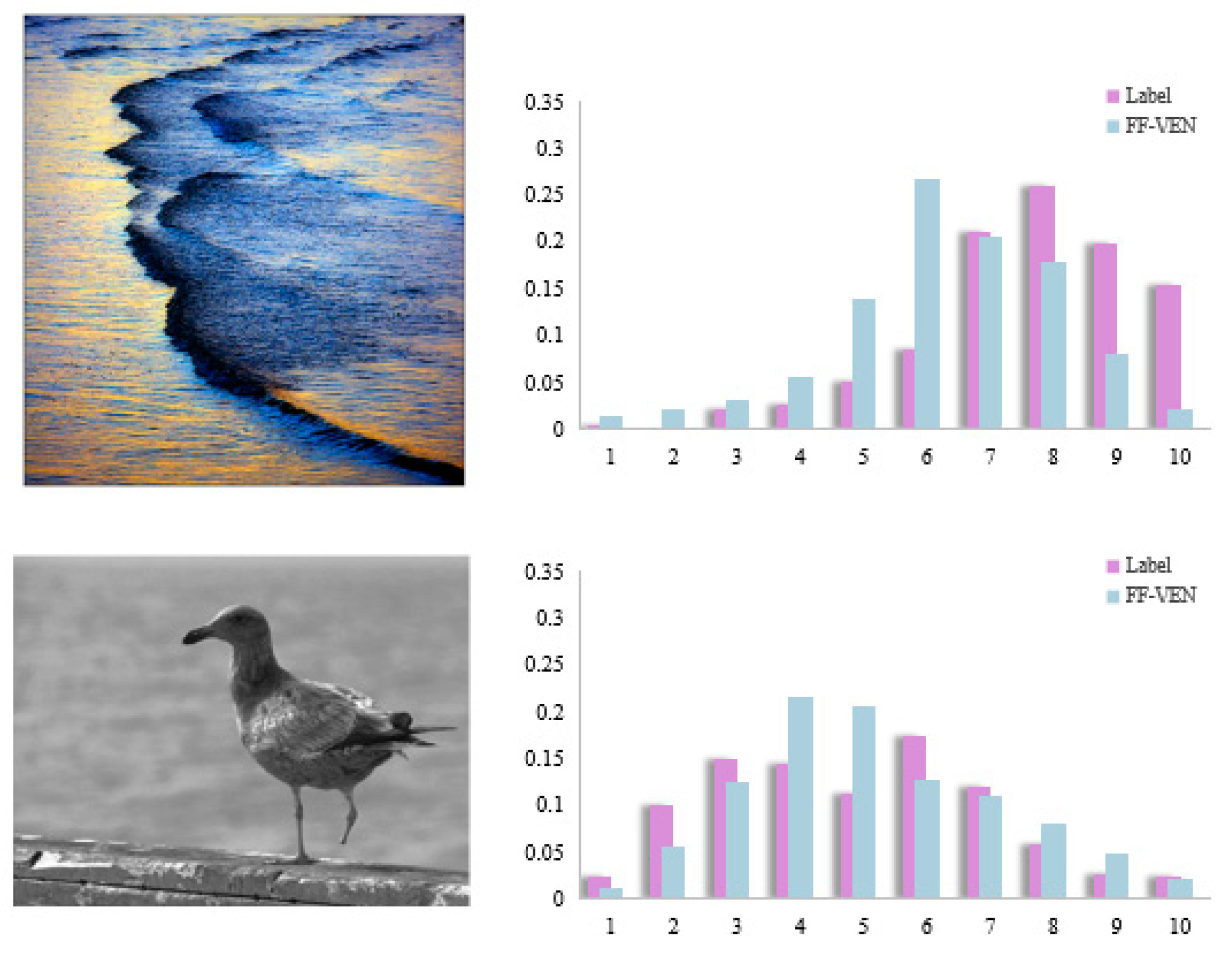
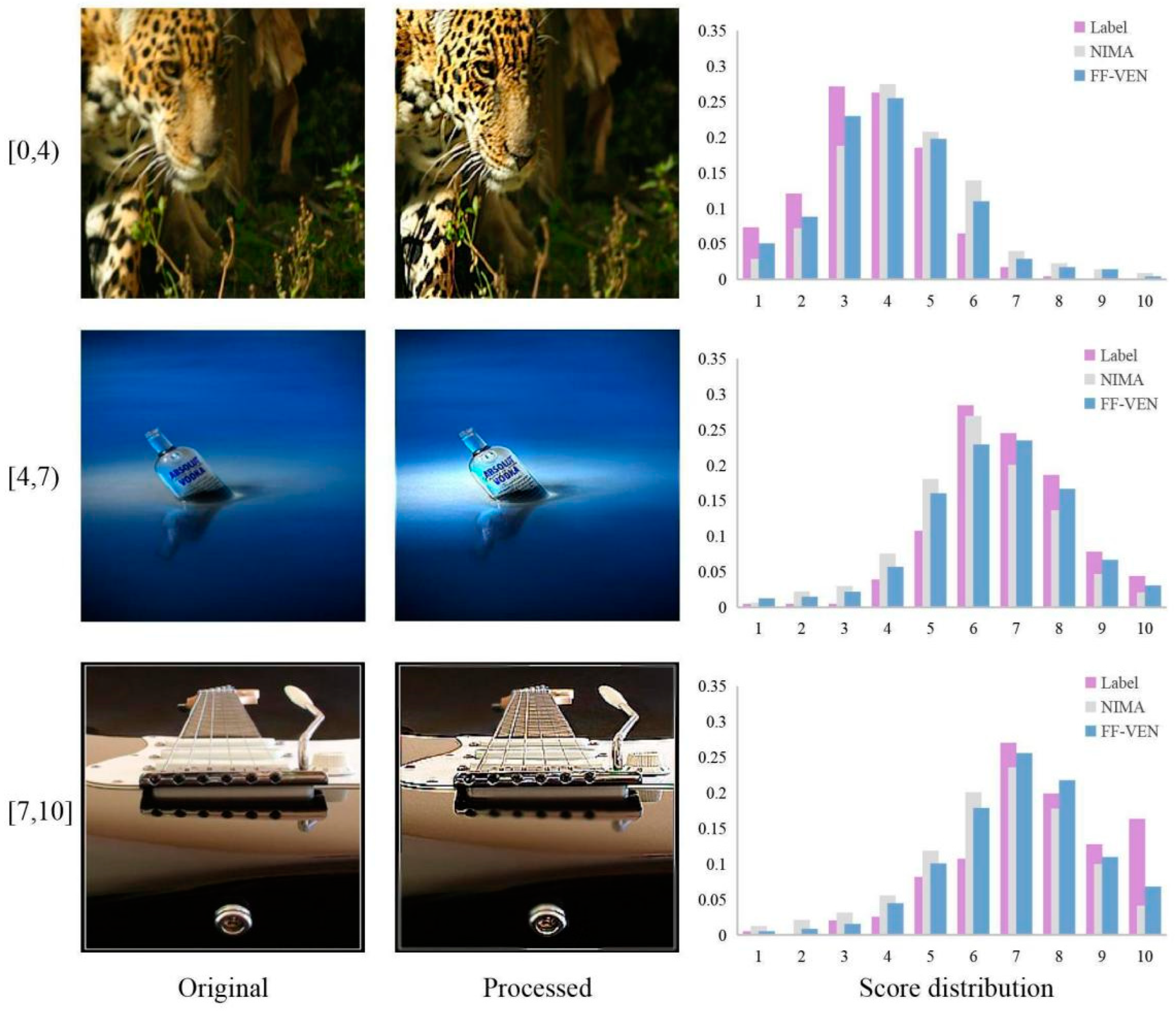
Figure 8 shows some examples of images with Mean in different intervals for comparison. It can be found that the difference between the distribution predicted by FF-VEN and that of the labels is smaller than the other two. Images with Mean in [7,10] are less controversial. Most people give these images high scores. The composition of professional images is abstract and artistic, which is difficult for CNN to learn. From the above experiments, it seems that VE module enhances the features of images based on human visual characteristics, leading to improving the prediction confidence of FF-VEN. Figure 9 shows some failure cases of FF-VEN. The network we trained does not perform well on images with very non-Gaussian distributions, like bimodal or very skewed distributions. However, the Gaussian functions perform adequately for 99.77% of all the images in the AVA dataset [15].
Figure 8. Some examples of the results of FF-VEN. Means of the images in Line 1, Line 2, and Line 3 are respectively in [0,4), [4,7), [7,10]. In Column 3, the magenta scores are the label distribution. The gray distribution is predicted by NIMA and the mazarine distribution is predicted by FF-VEN.
Preprints 72050 g008

4.7. Model Size Comparison

Timings of one pass of NIMA (VGG16) [8] models on an image of size 224×224×3 are 150.34ms (CPU) and 85.76ms (GPU). And it has 134.3 million parameters. In ReLIC++ [27], the attention map is of size 49×49. The training time cost of Full GoogLeNetV1-BN [21] is 16 days. The model size is 82.56 million. Training ILGNet-Inc.V1-BN [23] costs 4 days. In manuscripts, the model size of FF-VEN is 14.7 Million. Evidently, FF-VEN is significantly lighter than ReLIC++. SDFF module improves the model size by about 119.6 M, compared to NIMA (VGG16). Training FF-VEN costs 4 days, which is faster than Full GoogLeNetV1-BN. In general, FF-VEN is light-weight and achieves inspiring aesthetic prediction accuracy, as reported in Table 8.

5. Conclusion

FF-VEN proposed in this paper considers neural attention, human visual characteristics, and image understanding. It consists of VE module and SDFF module. According to ROI extracted by neural feedback, VE module not only selects the Laplace filter or GLPF but also adjusts the parameters of filters. It enables the computer to simulate human eyes assessing the digital images. SDFF module takes out the shallow feature and the deep feature via transverse connection, and fuses them on the basis of information contribution maximization. The results of comparison on AVA dataset and Photo.net dataset demonstrate the superiority of FF-VEN. In the future, we aim to analyze the network structure of ResNet, InceptionNet, and other CNN. To make the method more comprehensive, we attempt to focus on more factors, such as image themes, photography aesthetics, and human emotions.

Author Contributions

Methodology, X.Z.; Supervision, X.Z.; Validation, X.J.; Writing-original draft, X.J.; Formal analysis, Q.S.; Writing-review & editing, P.Z. All authors have read and agreed to the published version of the manuscript.

Funding Statement

This work was supported by National Key Research and Development Program of China (No. 2020AAA0108700).

Data Availability

We used publicly available datasets in order to illustrate and test our network. The AVA dataset can be found in http://www.dpchallenge.com/ and Photo.net dataset can be found in https://www.photo.net/.

Conflicts of Interest

The authors declare that they have no conflicts of interest.

References

  1. Yan, M.; Xiong, R.; Shen, Y.; Jin, C. Intelligent generation of Peking opera facial masks with deep learning frameworks. Herit. Sci. 2023, 11, 20. [Google Scholar] [CrossRef]
  2. Deng, Y.; Loy, C.C.; Tang, X. Image aesthetic assessment: an experimental survey. IEEE Signal Processing Magazine 2017, 34, 80–106. [Google Scholar] [CrossRef]
  3. Golestaneh, S.A.; Dadsetan, S.; Kitani, K.M. No-reference image quality assessment via transformers, relative ranking, and self-consistency. In Proceedings of the 2022 IEEE/CVF Winter Conference on Applications of Computer Vision (WACV), Waikoloa, HI, USA, 03-08 January 2022; pp. 3989–3999. [Google Scholar]
  4. Zhou, J.; Zhang, Q.; Fan, J.H.; Sun, W.; Zheng, W.S. Joint regression and learning from pairwise rankings for personalized image aesthetic assessment. Computational Visual Media 2021, 7, 241–252. [Google Scholar] [CrossRef]
  5. Yan, M.; Lou, X.; Chan, C.A.; Wang, Y.; Jiang, W. A semantic and emotion-based dual latent variable generation model for a dialogue system. CAAI Trans. Intell. Technol. 2023, 1–12. [Google Scholar] [CrossRef]
  6. Qian, Q.; Cheng, K.; Qian, W.; Deng, Q.; Wang, Y. Image Segmentation Using Active Contours with Hessian-Based Gradient Vector Flow External Force. Sensors 2022, 22, 4956. [Google Scholar] [CrossRef] [PubMed]
  7. Wang, D.; Zhang, H.; Shao, Y. A Robust Invariant Local Feature Matching Method for Changing Scenes. Wireless Communications and Mobile Computing 2021, 1–13. [Google Scholar] [CrossRef]
  8. Szegedy, C.; Vanhoucke, V.; Ioffe, S.; Shlens, J.; Wojna, Z. Rethinking the inception architecture for computer vision. In Proceedings of the 2016 IEEE Conference on Computer Vision and Pattern Recognition (CVPR), Las Vegas, NV, USA, 27-30 June 2016; pp. 2818–2826. [Google Scholar]
  9. Talebi, H.; Milanfar, P. NIMA: neural image assessment. IEEE Transactions on Image Processing 2018, 27, 3998–4011. [Google Scholar] [CrossRef]
  10. Simonyan, K.; Zisserman, A. Very deep convolutional networks for large-scale image recognition. Computer Science 2014, 1–14. [Google Scholar] [CrossRef]
  11. Saraee, E.; Jalal, M.; Betke, M. Visual complexity analysis using deep intermediate-layer features. Computer Vision and Image Understanding 2020, 195, 1–17. [Google Scholar] [CrossRef]
  12. Wang, P.; Cottrell, G.W. Central and peripheral vision for scene recognition: a neurocomputational modeling exploration. Journal of Vision 2017, 17, 1–22. [Google Scholar] [CrossRef]
  13. Ma, S.; Liu, J.; Chen, C.W. A-lamp: Adaptive layout-aware multipatch deep convolutional neural network for photo aesthetic assessment. In Proceedings of the 2017 IEEE Conference on Computer Vision and Pattern Recognition (CVPR), Honolulu, HI, USA, 21-26 July 2017; pp. 722–731. [Google Scholar]
  14. Zhang, X.; Gao, X.; Lu, W.; Yu, Y.; He, L. Fusion global and local deep representations with neural attention for aesthetic quality assessment. Signal Process.: Image Communication 2019, 78, 42–50. [Google Scholar] [CrossRef]
  15. Zhang, X.; Gao, X.; Lu, W.; He, L. A gated peripheral-foveal convolutional neural network for unified image aesthetic prediction. IEEE Transactions on Multimedia 2019, 21, 2815–2826. [Google Scholar] [CrossRef]
  16. Datta, R.; Joshi, D.; Li, J.; Wang, J.Z. Studying aesthetics in photographic images using a computational approach. In Proceedings of the 9th European Conference on Computer Vision (ECCV2006), Graz, Austria, 8-11 May 2006; pp. 288–301. [Google Scholar]
  17. Sun, X.; Yao, H.; Ji, R.; Liu, S. Photo assessment based on computational visual attention model. In Proceedings of the the 17th ACM international Conference on Multimedia, Beijing, China, 19-24 October 2009; pp. 541–544. [Google Scholar]
  18. Dhar, S.; Ordonez, V.; Berg T., L. High level describable attributes for predicting aesthetics and interestingness. In Proceedings of the 2011 Conference on Computer Vision and Pattern Recognition (CVPR), Colorado Springs, CO, USA, 20-25 June 2011; pp. 1657–1664. [Google Scholar]
  19. Bhattacharya, S.; Sukthankar, R.; Shah, M. A holistic approach to aesthetic enhancement of photographs. ACM Transactions on Multimedia Computing, Communications, and Applications 2011, 7, 1–21. [Google Scholar] [CrossRef]
  20. Tang, X.; Luo, W.; Wang, X. Content-based photo quality assessment. IEEE Transactions on Multimedia 2013, 15, 1930–1943. [Google Scholar] [CrossRef]
  21. Szegedy, C.; Liu, W.; Jia, Y.; et al. Going deeper with convolutions. In Proceedings of the 2015 IEEE Conference on Computer Vision and Pattern Recognition (CVPR), Boston, MA, USA, 07-12 June 2015; pp. 1–9. [Google Scholar]
  22. Lu, X.; Lin, Z.; Shen, X.; Mech, R.; Wang, J.Z. Deep multi-patch aggregation network for image style, aesthetics, and quality estimation. In Proceedings of the 2015 IEEE International Conference on Computer Vision (ICCV), Santiago, Chile, 07-13 December 2015; pp. 990–998. [Google Scholar]
  23. Jin, X.; Wu, L.; Li, X.; et al. ILGNet: inception modules with connected local and global features for efficient image aesthetic quality classification using domain adaptation. IET Computer Vision 2019, 13, 206–212. [Google Scholar] [CrossRef]
  24. Yan, G.; Bi, R.; Guo, Y.; Peng, W. Image aesthetic assessment based on latent semantic features. Information (Switzerland) 2020, 11, 1–17. [Google Scholar] [CrossRef]
  25. Zhang, X.; Gao, X.; Lu, W.; He, L.; Li, J. Beyond vision: a multimodal recurrent attention convolutional neural network for unified image aesthetic prediction tasks. IEEE Transactions on Multimedia 2020, 23, 611–623. [Google Scholar] [CrossRef]
  26. She, D.; Lai, Y.K.; Yi, G.; Xu, K. Hierarchical layout-aware graph convolutional network for unified aesthetics assessment. In Proceedings of the 2021 IEEE/CVF Conference on Computer Vision and Pattern Recognition (CVPR), Nashville, TN, USA, 20-25 June 2021; pp. 8471–8480. [Google Scholar]
  27. Zhao, L.; Shang, M.; Gao, F.; Li, R.; Yu, J. Representation learning of image composition for aesthetic prediction. Computer Vision and Image Understanding 2020, 199, 103024. [Google Scholar] [CrossRef]
  28. Zhang, J.; Bargal, S.A.; Zhe, L.; Brandt, J.; Shen, X.; Sclaroff, S. Top-down neural attention by excitation backprop. International Journal of Computer Vision 2018, 126, 1084–1102. [Google Scholar] [CrossRef]
  29. Kucer, M.; Loui, A.C.; Messinger, D.W. Leveraging expert feature knowledge for predicting image aesthetics. IEEE Trans. Image Processing 2018, 27, 5100–5112. [Google Scholar] [CrossRef]
  30. Zhang, R.; Isola, P.; Efros, A.A.; Shechtman, E.; Wang, O. The unreasonable effectiveness of deep features as a perceptual metric. In Proceedings of the 2018 IEEE/CVF Conference on Computer Vision and Pattern Recognition, Salt Lake City, UT, USA, 18-23 June 2018; pp. 586–595. [Google Scholar]
  31. Jin, X.; Wu, L.; Song, C.; et al. Predicting aesthetic score distribution through cumulative jensen-shannon divergence. In Proceedings of the AAAI Conference on Artificial Intelligence (AAAI), New Orleans, Louisiana, USA, 2-7 February 2018; pp. 77–84. [Google Scholar]
  32. Murray, N.; Marchesotti, L.; Perronnin, F. AVA: a large-scale database for aesthetic visual analysis. In Proceedings of the 2012 IEEE Conference on Computer Vision and Pattern Recognition, Providence, RI, USA, 16-21 June 2012; pp. 2408–2415. [Google Scholar]
  33. Joshi, D.; Datta, R.; Fedorovskaya, E.; et al. Aesthetics and Emotions in Images. IEEE Signal Processing Magazine 2011, 28, 94–115. [Google Scholar] [CrossRef]
  34. He, K.; Zhang, X.; Ren, S.; Sun, J. Spatial pyramid pooling in deep convolutional networks for visual recognition. IEEE Transactions on Pattern Analysis and Machine Intelligence 2015, 7, 1904–1916. [Google Scholar] [CrossRef] [PubMed]
  35. Zeng, H.; Zhang, L.; Bovik, A.C. A probabilistic quality representation approach to deep blind image quality prediction. CaRR 2017, 1–12. [Google Scholar] [CrossRef]
  36. Wang, W.; Shen, J.; Ling, H. A Deep Network Solution for Attention and Aesthetics Aware Photo Cropping. IEEE Transactions on Pattern Analysis and Machine Intelligence 2018, 4, 1531–1544. [Google Scholar] [CrossRef]
  37. Marchesotti, L.; Perronnin, F.; Larlus, D.; Csurka, G. Assessing the aesthetic quality of photographs using generic image descriptors. In Proceedings of the 2011 International Conference on Computer Vision, Barcelona, Spain, 06-13 November 2011; pp. 1784–1791. [Google Scholar]
  38. Hao, Y.; He, R.; Huang, K. Deep aesthetic quality assessment with semantic information. IEEE Transactions on Image Processing 2017, 26, 1482–1495. [Google Scholar] [CrossRef]
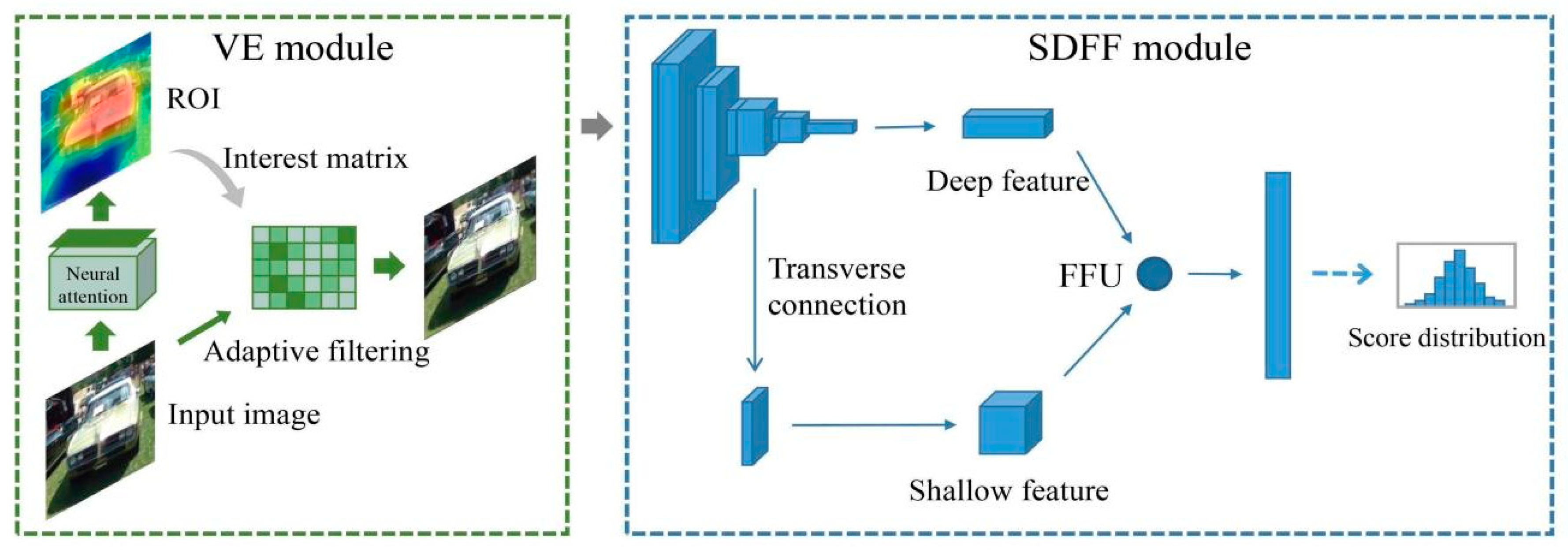
Figure 1. The overall framework of FF-VEN. VE module filters images adaptively based on ROI. SDFF module uses FFU to fuse the shallow feature and the deep feature extracted by the method of transverse connection. Finally, the score distribution is directly predicted.
Preprints 72050 g001
Figure 2. The examples of images with ROI. We apply pseudo-color technique to the interest matrix (JET mapping). The colors are red, orange, yellow, green, blue and purple in turn. Red indicates the highest degree of interest and purple represents the lowest degree of interest.
Preprints 72050 g002
Figure 3. The process of adaptive filtering. The adaptive filter analyzes the interest degree in each pixel depending on the extracted interest matrix. GIPF or Laplace filter is dynamically selected to simulate human eyes.
Preprints 72050 g003
Figure 4. The examples of adaptive filtering. Column 1, the original images; Column 2, the results of adaptive filtering; Column 3, the processed images.
Preprints 72050 g004
Figure 5. The feature's understanding of an image in VGG16. The information contained in the features is attached to the original image with the incentive support method. It is confident for the deep feature to recognize objects. The shallow feature captures the foreground by learning low-level information.
Preprints 72050 g005
Figure 6. The framework of FFU. PCFS analyzes the contribution of features. Meanwhile, features pass through the max pooling layer and the average pooling layer, respectively. FFU dot pooled features with their weights and then fuse the results via the catenation layer. The gray dotted box represents the process of analyzing the contribution without changing the features numerically.
Preprints 72050 g006
Figure 9. Some examples of the failure cases.
Preprints 72050 g009
Table 1. The parameters in the adaptive filter.
Filter size k b σ
The high-boost filter (including Laplace filter) 9×9 i t h r e s h o l d M a x t h r e s h o l d 2 i t h r e s h o l d -
Gaussian filter 9×9 - - t h r e s h o l d i t h r e s h o l d M i n
Table 2. The main parameters of VGG16.
Layer a The size of input data The number of the layer
Conv3-64 224x224x3 2
Conv3-128 112x112x64 2
Conv3-256* 56x56x128 3
Conv3-512 28x28x256 3
Conv3-512* 14x14x512 3
a The layers from Line 1 to Line 5 are the convolution layer of VGG16. The asterisk * represents the layer that we take out the feature from.
Table 3. The main parameters of FFU.
Layer The size of input data The number of the layer
PCFS 28x28x256,7x7x512 1
FC 7x7x256+7x7x512 1
Table 4. The results of comparison on AVA dataset.
Network architecture Accuracy
(%)
LCC
(mean)
SRCC
(mean)
MAE RMSE EMD
SPP-Net [34] 74.41 0.5869 0.6007 0.4611 0.5878 0.0539
AA-Net [35] 77.00 - - - - -
InceptionNet [7] 79.43 0.6865 0.6756 0.4154 0.5359 0.0466
NIMA [8] 81.51 0.636 0.612 - - 0.050
GPF-CNN [15] 81.81 0.7042 0.6900 0.4072 0.5246 0.045
ReLIC++ [27] 82.35 0.760 0.748 - - -
FF-VEN 83.64 0.773 0.755 0.4011 0.5109 0.044
Table 5. The results of comparison on Photo.net dataset.
Network architecture Accuracy
(%)
LCC
(mean)
SRCC
(mean)
MAE RMSE EMD
GIST-SVM [37] 59.9 - - - - -
FV-SIFT-SVM [37] 60.8 - - - - -
MRTLCNN [38] 65.2 - - - - -
GLFN [14] 75.6 0.5464 0.5217 0.4242 0.5211 0.070
FF-VEN 78.1 0.6381 0.6175 0.4278 0.5285 0.062
Table 6. The results of comparison on AVA dataset.
Network architecture Accuracy
(%)
LCC
(mean)
SRCC
(mean)
MAE RMSE EMD
VGG16 [36] 74.41 0.5869 0.6007 0.4611 0.5878 0.0539
Random-VGG16 [20] 78.54 0.6382 0.6274 0.4410 0.5660 0.0510
Saliency-VGG16 [38] 79.19 0.6711 0.6601 0.4228 0.5430 0.0475
GPF-VGG16 [15] 80.70 0.6868 0.6762 0.4144 0.5347 0.0460
VE-CNN (VGG16) 81.03 0.7395 0.7185 0.4073 0.5279 0.0441
SDFF (VGG16) 81.47 0.7119 0.7021 0.4103 0.5317 0.0462
Table 7. Evaluation results for images with Mean in different intervals.
Mean Network architecture Accuracy
(%)
LCC
(mean)
SRCC
(mean)
MAE RMSE EMD
NIMA [8] 78.46 0.6265 0.6043 0.5577 0.6897 0.067
[0,4) ReLIC++ [27] 80.02 0.6887 0.6765 - - -
FF-VEN 80.59 0.7095 0.6971 0.5037 0.6139 0.059
NIMA [8] 80.43 0.7271 0.7028 0.4037 0.5256 0.048
[4,7) ReLIC++ [27] 81.15 0.8733 0.8547 - - -
FF-VEN 81.33 0.8945 0.8831 0.3748 0.4851 0.039
NIMA [8] 94.93 0.5936 0.5645 0.5927 0.7314 0.073
[7,10] ReLIC++ [27] 96.64 0.6223 0.6084 - - -
FF-VEN 98.71 0.6113 0.6492 0.5343 0.6457 0.061
Table 8. Comparison of model size.
Model Size
NIMA(VGG16) [8] 134.3 M
GoogLeNet [21] 82.36 M
ReLIC++ [27] 17.51M
FF-VEN 14.7 M
Disclaimer/Publisher’s Note: The statements, opinions and data contained in all publications are solely those of the individual author(s) and contributor(s) and not of MDPI and/or the editor(s). MDPI and/or the editor(s) disclaim responsibility for any injury to people or property resulting from any ideas, methods, instructions or products referred to in the content.
Copyright: This open access article is published under a Creative Commons CC BY 4.0 license, which permit the free download, distribution, and reuse, provided that the author and preprint are cited in any reuse.
Prerpints.org logo

Preprints.org is a free preprint server supported by MDPI in Basel, Switzerland.

Subscribe

© 2024 MDPI (Basel, Switzerland) unless otherwise stated