Preprint
Article

Variable Speed Control in PATs: Theoretical, Experimental and Numerical Modelling

Altmetrics

Downloads

114

Views

23

Comments

0

A peer-reviewed article of this preprint also exists.

Submitted:

28 April 2023

Posted:

28 April 2023

You are already at the latest version

Alerts
Abstract
pump as turbine (PAT); computational fluid dynamics; variable rotational nominal speed; OpenFoam.
Keywords: 
Subject: Engineering  -   Civil Engineering

1. Introduction

The availability of water resources at the global level has significantly decreased. Among the main agents that have caused this situation are climate change, environmental pollution, human activities, and failures in hydraulic structures, among others. It is becoming increasingly complicated to access appropriate sources that meet the quality and quantity of the resource. Despite this, water loss due to leaks in pressurized distribution systems still manages considerable values, with losses of 8% to 24% in developed countries [2]. If it is considered that the need for water is increasing, there is an urgent need to implement sustainable projects that allow the user to be carried out efficiently[3]. This type of project requires the use and development of new technologies that are easy to implement and apply[4].
In the case of sustainable water systems, there are some approaches from which improvements can be proposed. Among these approaches are the determination of water quality parameters [5], optimization of energy efficiency [6,7]reduction of water leaks [8,9], mathematical modelling of management, and optimization of systems [10,11], among others.
Water distribution systems are not energy efficient because they depend on pressure demands that can generate leaks, increasing energy costs [12]. One of the elements that have a negative effect from the point of view of energy efficiency, but is necessary for the hydraulic operation of the systems is the pressure-reducing valve (PRV) [13]. PRVs are used to reduce the pressure at one point by regulating the flow passage. An alternative to the use of these devices, to reduce dependence on non-renewable energy[14]and take advantage of the excess energy of these systems [15], is the use of PATs (Pumps working as a turbine). In addition, PATs have been used as energy-generating devices in micro-hydroelectric power plants as a sustainable solution in the water industry[16]. For this reason, it is a trend to study the use of PATs to optimize different water systems to improve their sustainability [17,18,19].
PATs are pumps that work in reverse mode to generate energy. This machine's cost is cheaper than a conventional turbine of the same size[20], although they have lower hydraulic efficiencies in ranges between 0.6 and 0.7 [21]. When all electromechanical equipment is considered, the overall efficiency decreases to values between 0.5 to 0.6 [1]. The use of pumps operating as turbines (PATs) increases due to their application, availability, and cost advantages [7,22,23,24,25,26,27]. For example, Novara et al. [28]conclude that an installation with PATs could be 5 to 15 times cheaper than a conventional installation with turbines.
The PATs study begins with Thoma and Kittredge [29], who accidentally found that pumps can operate efficiently as turbines when trying to evaluate the complete characteristics of the pumps. In 1957, Stepanoff [30] reported several modes of operation of the pumps on performance curves plotted in quadrants. Once it was discovered that PATs could be applied in the chemical industry and the supply of drinking water, different researchers developed some techniques to predict the operation of this type of machine. In 1962 Childs [31] carried out comparative studies between efficiencies in devices working in both modes (pump-turbine). Subsequently, the first studies were carried out to predict the performance values in turbine mode and get the Best Efficient Point (BEP) through linear equations. The PATs study has been developed with different approaches, such as in water distribution systems, where Jain's [32] research stands out the results of placing PATs in distribution systems. Fecarotta [33] y Morani [12] proposes an analysis regarding the proper location of PATs; the latter focuses its research looking for cost reduction and maximization of production and energy savings. Moazeni [34] investigates finding the optimal number and location of PATs through mixed nonlinear programming models. Macias [19] established a methodology that was applied in an irrigation project in a rural area in the province of Valencia (Spain) that focuses on optimizing the location and selection of PATs based on the influence of leaks. The same author [14] develops a new methodology for self-calibration of leaks to know the injected flow rate and the volume consumed in the water networks. This methodology was applied in the city of Manta, Ecuador.
Since the performance curves are not available in pumps that work in turbine mode [27], different studies and methodologies have been carried out to obtain them, and to select the appropriate machine depending on the type of working condition required. Rossi [35] proposes a general method to predict PATs performance using artificial neural networks (ANN). Based on the datasheets provided by the pump manufacturers, the author obtains the BEP and off-design performance using the ANN methodology. In addition, the resulting predictions were compared with experimental data not used in the training process, which resulted in a high degree of compatibility. The study concluded that the BEP flow rate increases in reverse mode while the specific speed in BEP decreases slightly and also recommends the use of this tool to choose the proper PAT. To estimate the BEP and the characteristic curves of the PATs, Perez-Sánchez [21] proposed new approach equations from an experimental base of 181 machines. In the same sense, Plua [1] presents new empirical expressions to estimate head, efficiency, and power curves for PATs with variable speed. These equations allow the application of various operation strategies in hydraulic simulation tools (e.g., Epanet, WaterGEMS).
Micro hydroelectric power plants (MHP) have become very effective solutions for rural sectors with powers of 5-100 kW. The big problem with these facilities is the high turbine cost concerning the entire project [27]. In the case of MHP, the price of these elements can be higher than 60%–70% [36]. One possibility to reduce this cost is to use PATs instead of a conventional turbine [37], which would favour the expansion of MHP and the reduction of greenhouse gas emissions [28]. In 2012 Pascoa [38]proposed a new approach for a hydroelectric plant with PAT with constant flow. Rossi [39]suggested the economic feasibility of placing PATs in the Merano aqueduct, which resulted in the production of 338 kWh of daily electricity and power of 19.18 kW. Table 1 [27]shows different PATs installations in power generation projects.
CFD techniques have been widely used to predict characteristic curves and performance of pumps in direct and reverse modes and proved to be an effective solution in PATs approaches [40,41,42,43]. Also, an experimental investigation is fundamental for obtaining reliable results in PATs under different optimization stages [1,15,44,45]. Different types of machines such as axial, mixed, and radial PATs; with horizontal and vertical axis; single and multistage [46], have been studied using CFD simulations for fixed and variable speeds [24,25,26]. However, very few studies related to numerical modelling in PATs of variable rotational speed have been executed, so it is imperative to establish equations and laws that predict their behaviour [47]. The numerical simulations were carried out to define the performance of the pump [48], analyze flow in turbine mode [49], predicting and extrapolate characteristic curves [50], among others.
Plua [40] presented research in which the main parameters and techniques that have been simulated for PATs through CFD are shown and whose main simulation ranges are mentioned: specific speed: 0.8 -306; rotational speed: 250-3900 rpm; flow rate: 2.9-300 l/s; mass flow: 13-17.8 kg/s. Concerning numerical simulations, the principal turbulence models used were Reynolds Average Navier Stokes (RANS) and Unsteady Reynolds Average Navier Stokes(URANS). The most used closure model was k-e, followed by k-w and k-w-SST, among others. Regarding packages, ANSYS-CFX was the most used, followed by CFD Code Fluent and OpenFOAM. Respecting mesh generation, the number of cells was 1x10⁶ to 4.2x10⁶, with hexahedral, tetrahedral, mixed blocks, and pyramids. Depending on each situation, boundary conditions such as total pressure, mass flow rate, stagnation pressure, constant total pressure, static pressure, and volumetric flow were placed at the inlet and outlet of the model. In conclusion, it was established that the CFD methodology to predict the performance of a pump working as a turbine presented adequate accuracy based on the comparison of results with the experimental tests. However, numerous errors were also reported in some studies. The authors assumed that the reported errors are due to the geometries between the tests and the simulations not being identical, the loss estimation is not exact, and more experience in computational analysis is required for modelling this type of phenomenon. Finally, the same author [47] evaluated the application of numerical CFD simulation in PATs in comparison with experimental results and obtained conclusions for future numerical analysis. As a result, it was evidenced that there are few simulated cases where flow with variable speed is simulated and that the number of studies with free code computational packages is minimal, and that its use should be promoted due to its outstanding capabilities.
Therefore, the present study is focused on a numerical simulation in the OpenFOAM 3D free code package of PATs that have experimental data to validate the use of the new empirical expressions proposed for machines with different rotational speeds. The particularity in the modelling is that the study of a rotating PAT at different speeds will be carried out, and comparisons will be made with experimental results obtained on a test bench to calibrate the model.

2. Materials and Methods

Figure 1 depicts the main tasks performed to determine the validity of new expressions obtained by Plua [1] to predict the behaviour of PATs with variable speed:

2.1. Preprocess

2.1.1. Computational Domain

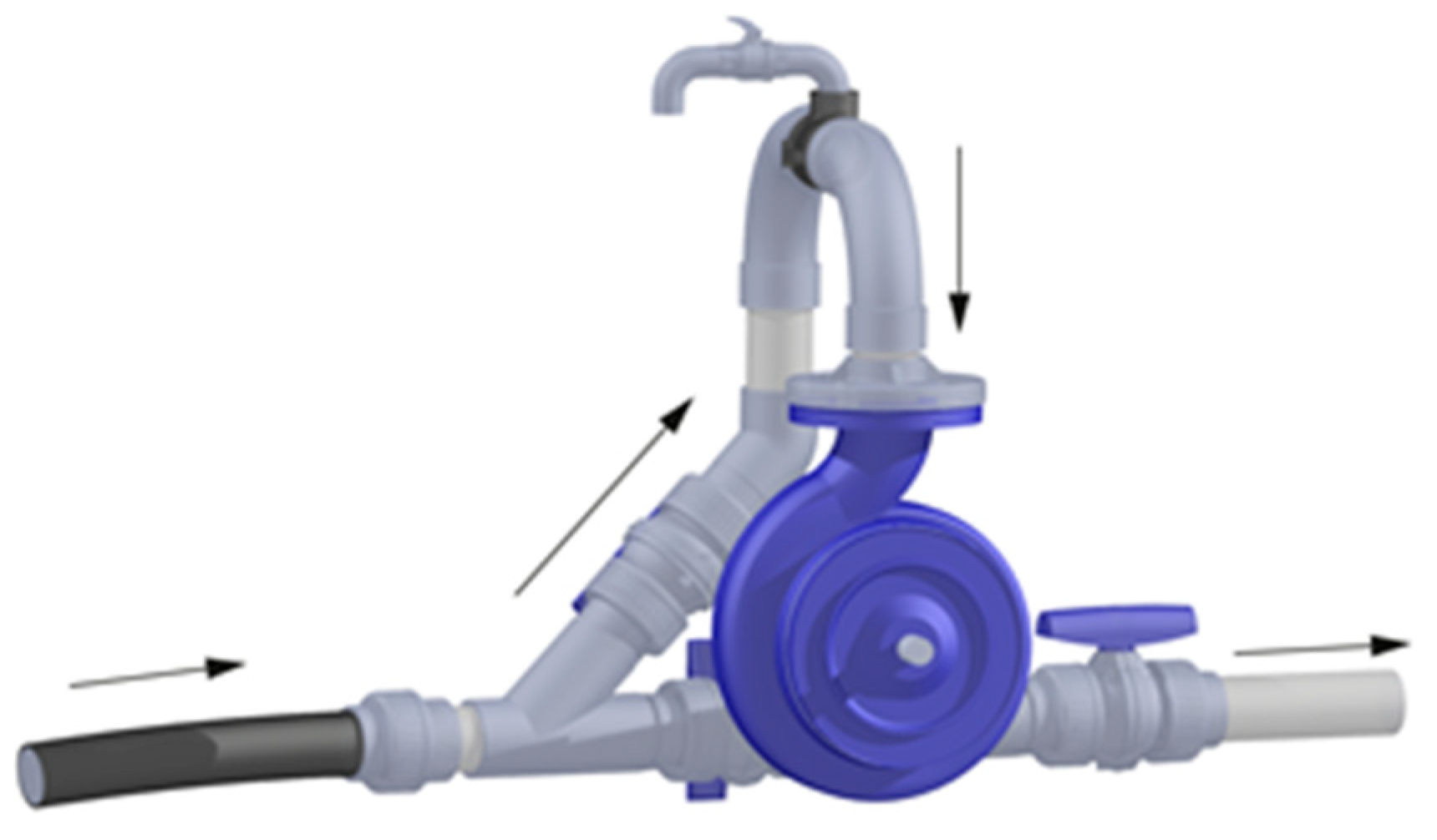
The PAT model presented in this study was taken from research conducted by Pérez Sánchez [51] and experimentally tested at the CERIS-Hydraulic Lab of Instituto Superior of Lisbon. Geometry corresponds to an installation of a PAT in a laboratory that allows experiments where flow, pressure conditions, and rotational speed can be varied. The hydraulic facility consists of a 1m3 air-vessel tank, a 50 mm HDPE pipe, a KSB radial impeller centrifugal pump (model Etarnom 232) that operates in turbine mode, regulating tank, pressure transducers, valves, and a flow recirculation pump. The air-vessel tank sends water to reach the PAT, which finally discharges to the open free surface tank and then incorporates it into the system through the recirculation pump. The 3D model was built in SolidWorks CAD system from which the following drawing view is extracted, see Figure 2.
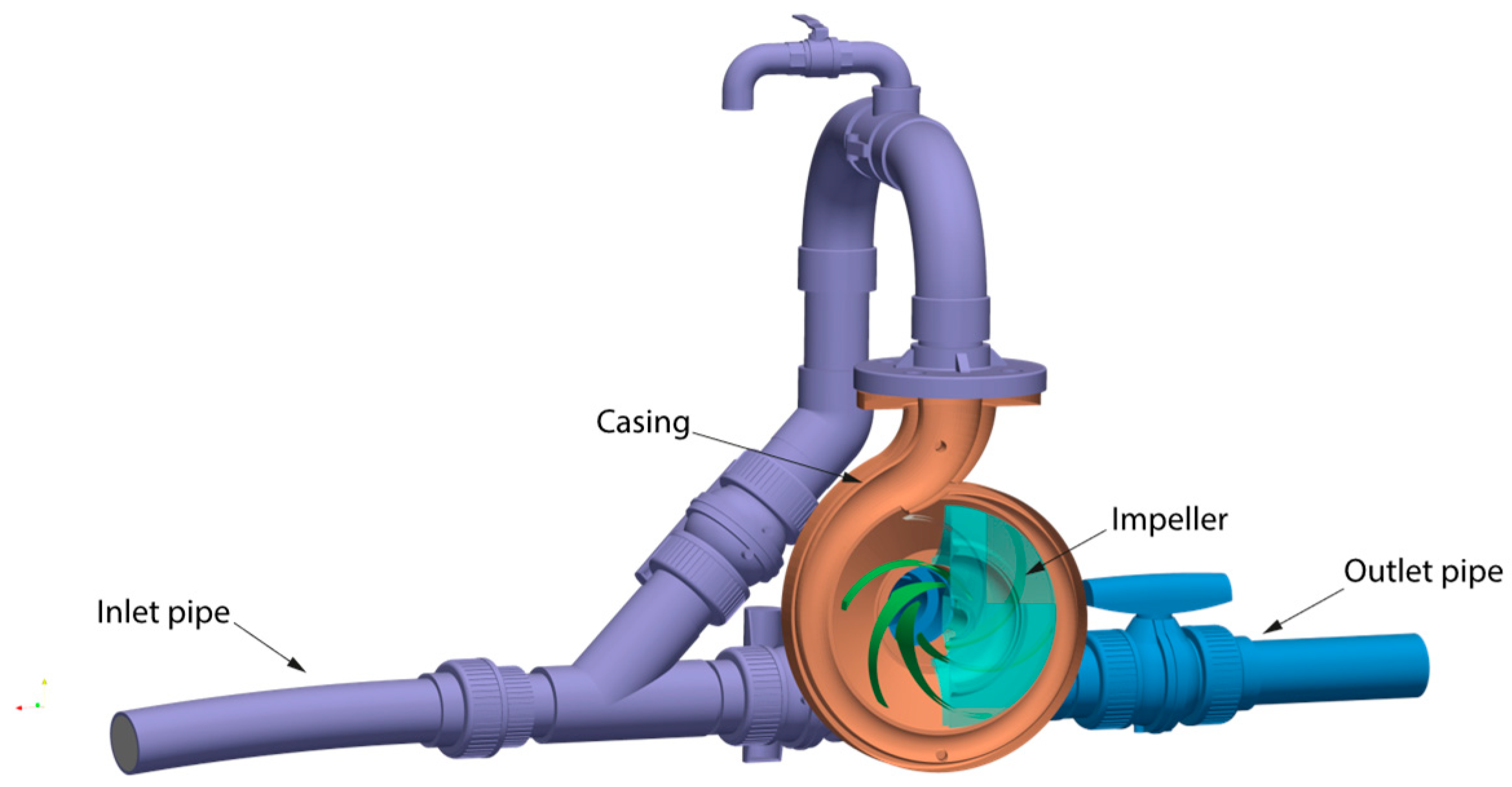
The computational domain consists of four parts: Inlet pipe starting in the inlet section and reaching the pump's runner, rotating part that is the impeller of PAT, rotating part of the domain; Casing, stationary part of the pump and; Outlet pipe, which corresponds to the discharge of the pump to the outlet. The original geometry was redefined according to the configuration of the control volumes to obtain optimal meshing. See Figure 3.
Depending on the actual geometry and its characteristics, the .stl files were modified with the Autodesk Inventor Software to get a better-quality mesh. The areas of meshing interest were prioritized: the casing, the impeller, and the blades. Each has different elements and details simultaneously with different levels and definition angles. It allows the surfaces to stick more to the edges, bringing the mesh's geometry closer to the actual configuration. The geometries modelled were the volute, the discharge pipe, the inlet pipe, and the impeller. In the case of the impeller, it was divided into three parts, as seen in Figure 3. The impeller is composed of the lower and upper parts and the blades. These elements are treated independently to improve the mesh quality and then facilitate the visualization of results at the post-processing stage. In addition, six blades were configured inside the impeller, which allows a better study of the phenomenon presented in the PAT.

2.1.2. Mesh

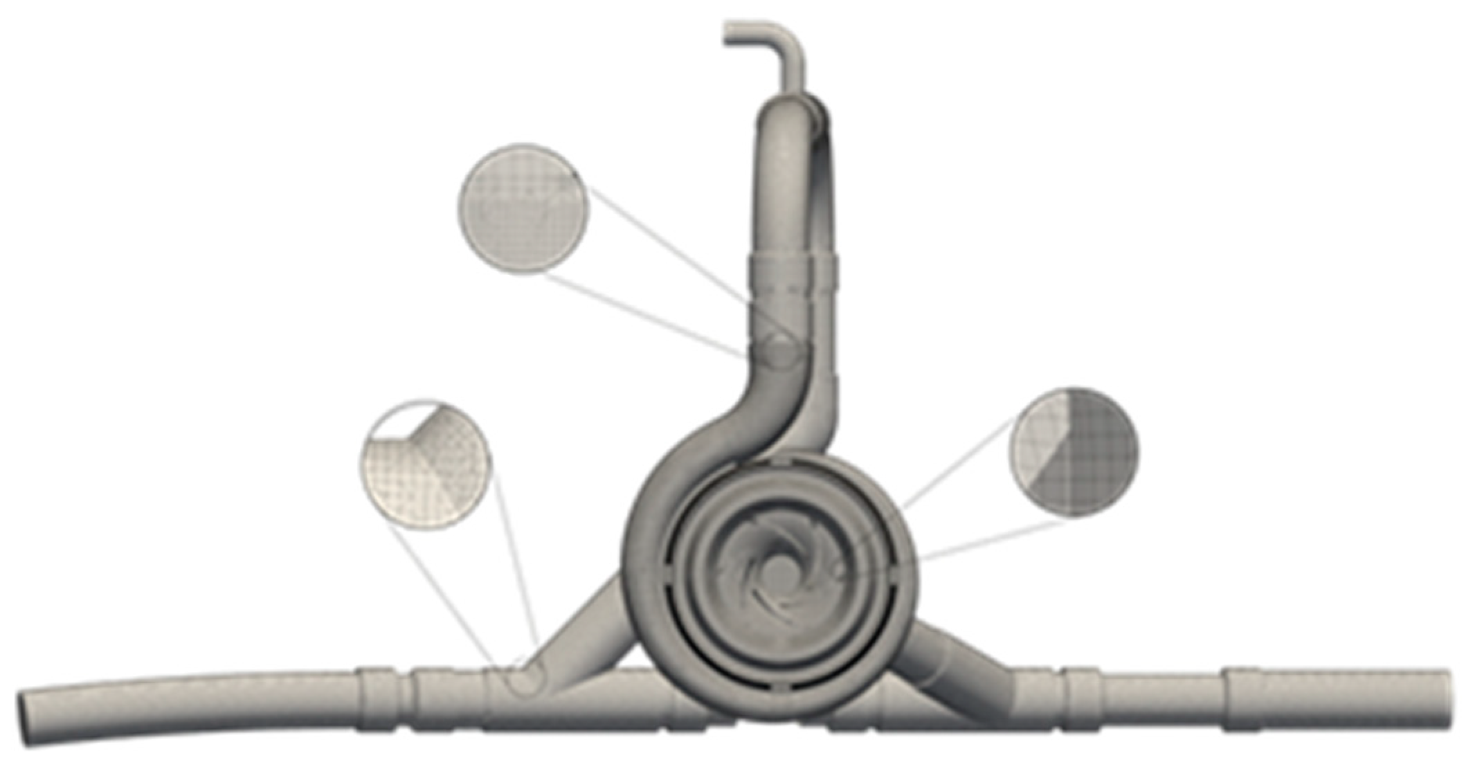
The mesh was created with snappy Hex Mesh, an automatic mesh generator that adjusts to the surface to obtain the required mesh. First, the 3D model was exported to the format.stl through Autodesk® Inventor® software. Later, with the help of HELIX-OS, the BlockMeshDict file was created to generate through BlockMesh utility orthogonal mesh elements for the Casing, Inlet pipe, Impeller, and Outlet, respectively. Once the block meshing was ready, the domain geometries were admitted in the snappyHexMeshDict file. The local refinement was defined through castellatedMesh, and the internal points within the closed domain were entered. Finally, it was necessary to use the topoSet tool to generate zones with movable cells for the runner and merge the meshes with the mergeMeshes utility. Mesh characteristics are presented in Table 2, and generated mesh is in Figure 4.

2.1.3. Approach

MRF Technique (Multiple Reference Frame) is the technique used for modelling rotation in CFD in this case. This methodology establishes a separate reference frame for each region of the domain, for both rotational and static [49]. It is based on the creation of a local region around the rotating object where the relative velocity is determined for each point. First, Navier Stokes equations are built, taking account of centrifugal and Coriolis forces, and then, a set of equations for stationary and rotational regions are created. This technique can accurately capture instantaneous local flow, which depends on the relative position of the rotative element versus static geometry. In the MRF approach, the Navier-Stokes equations are solved in terms of the global/inertial velocity. Since, in this case, there is a separation between the impeller and the scroll, the AMI approach is not applicable. For that reason, a set was used that allows simulation these elements in the MRF approach.

2.1.4. Boundary and Initial Conditions

Initial and boundary conditions should be applied when solving the Navier-Stokes and continuity equations. Table 3 summarizes the initial conditions related to the turbulence models used of this research. For the calibration of the mathematical model, the k-e turbulence model was used (the same one used by [51]). k is turbulent kinetic energy, and e is turbulent dissipation rate. The k-w(specific turbulent dissipation rate)-SST turbulence model was used to analyze the experimental data, the nominal rotational speed curve, and the results of the new expressions contained in [1].
The turbulent kinematic viscosity value “nut” represents the roughness in the walls confirming the domain. Regarding boundary conditions, a constant velocity input condition and a static pressure output condition were used. The boundary conditions of the computational domain are detailed in Table 4.

2.2. Numerical Simulation

2.2.1. CFD

The Navier-Stokes equations were solved using CFD methods based on a continuum mechanics approach for fluid mechanics to define the fluid behaviour in the PATs [50]. For that, two equations were considered that obtain the values of velocity and pressure that allow for defining the average behaviour of the flows. The equations correspond to the conservation of mass and linear momentum and are indicated in a tensor with the following expressions:[47]:
Preprints 72124 i001(1)
Preprints 72124 i002(2)
where i and j are subscripts for the three axes of space respectively, u ¯ is the filtered velocity magnitude, P ¯ is the filtered pressure, the subgrid stress tensor is T ¯ i j , and T ¯ i j the filtered viscous stress tensor.

2.2.2. CFD and Solvers

The CFD package used is the CFD OpenFOAM 9 which models multiphysics simulations applicable to Computational Fluid Dynamics for incompressible and compressible flows with application in dynamic mesh management to make rotating reference frames with adaptable mesh refinements as required. OpenFOAM uses a directory structure to solve the cases, where the case is the name of the analysis case; the system sets the numerical control to run time and solver; the constant contains the physical properties, modelling and mesh information; 0 has the edge conditions as well as the beginning to modelling and, time-directories that correspond the solutions and derived cases.
Regarding meshing, OpenFOAM has some mesh utilities such as BlockMesh, SnappyHexMesh, foamyHexMesh, and foamyQuadmesh. OpenFOAM also allows the mesh to be generated with other packages since mesh conversion utilities are compatible with popular mesh formats (Gmsh, Fluent, Ideas, and Netgen, among others). As stated above, SnappyHexMesh generated the mesh. SnappyHexMesh utility is an automatic hybrid mesh that divides, refines, and adjusts to the analyzed surface, attaching the mesh with complex details of geometry [52]
For the calibration of the model, the solver simpleFoam was applied to steady-state incompressible flow based on the SIMPLE (Semi-Implicit Method for Pressure Linked Equations) algorithm for pressure velocity-coupling [54] with applications in turbulent and transient flows in pipes.

3. Results

3.1. Numerical simulation validation

3.1.1. Mesh quality

The checkMesh tool was used to evaluate the mesh quality, giving the mesh stats, the overall number of cells of each type, topology, geometry, and conclusions about the mesh. Two parameters are used to verify the quality of the mesh; one of them is Ω, which corresponds to the following expression Ω =NE/ND, where ND is the number of nodes and NE is the number of elements.Ω indicating the homogeneity of the mesh, a good mesh quality will present Ω values close to 1, and values close to 2 have very dispersed meshes. For this case study, the calculated Ω value is 0.69, which is acceptable. The other value is the so-called y+ which verifies the acceptable range of values for the turbulence model. If this value is less than 1, it is considered that the quality of the mesh is good. In this study, it was found that the average y+ values in all the simulations of the mesh are less than 1.

3.1.2. Calibration

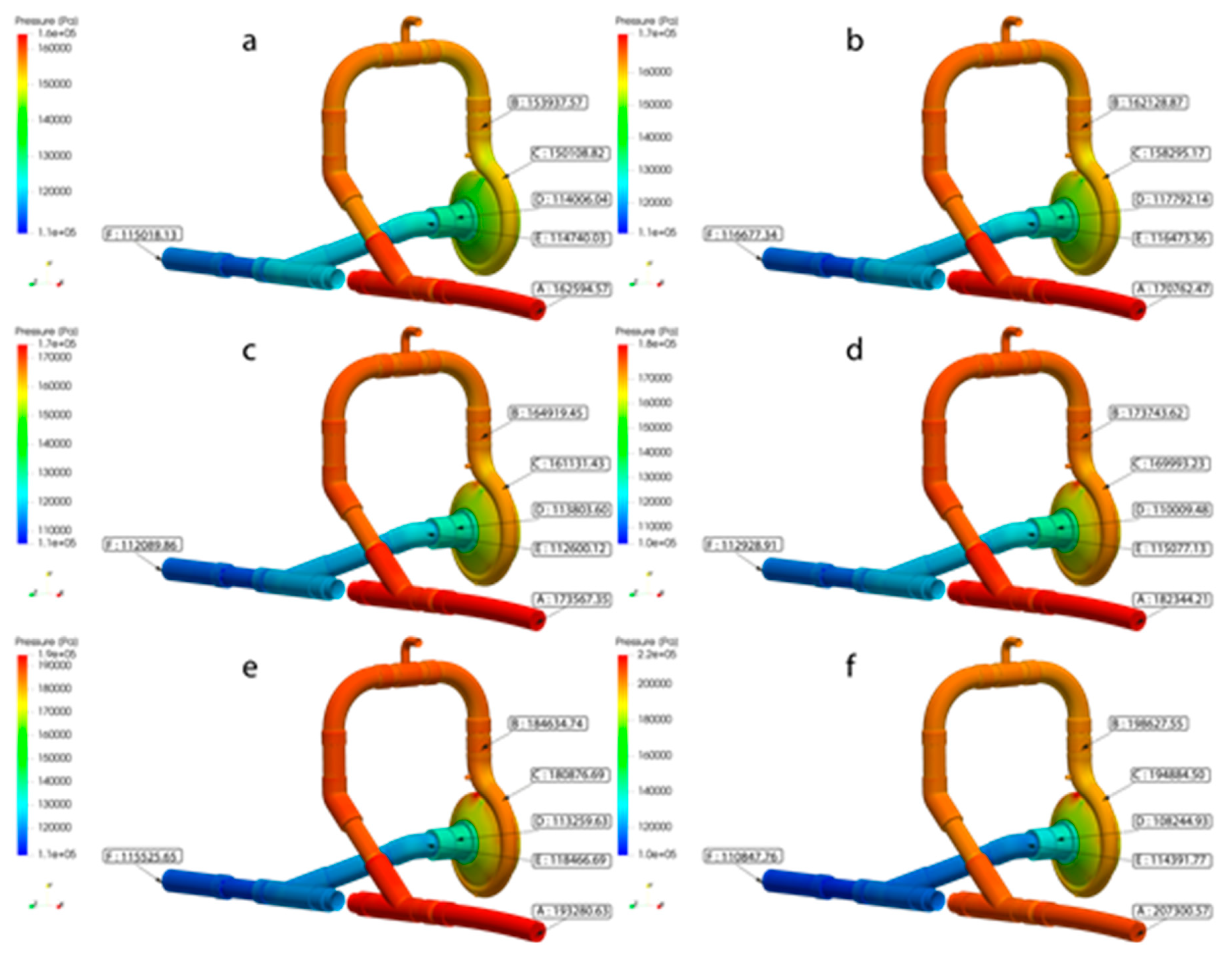
For the CFD simulation validation, two calibrations were performed concerning the Pérez-Sánchez study [51]. The first concerns the mathematical model made with SolidWorks-FloEFD and the second concerns experimental research. In the Pérez-Sánchez CFD model, the simulated global variables were: the head (H), the output hydraulic torque (T), the discharge (Q), and the rotational speed (N). Within the simulations, the absolute static pressure contours were obtained for a flow rate of 4.5 l/s and rotation speeds of 810rpm, 930rpm, 1050rpm, 1170rpm, 1275rpm, and 1500rpm. The results show that the pressure decreases from upstream to downstream as the fluid flows within the domains and along the impeller, from the inner to the outer region, as the energy is transmitted to the shaft. On the other hand, it was found that the higher the speed, the lower the pressure value downstream of the impeller.
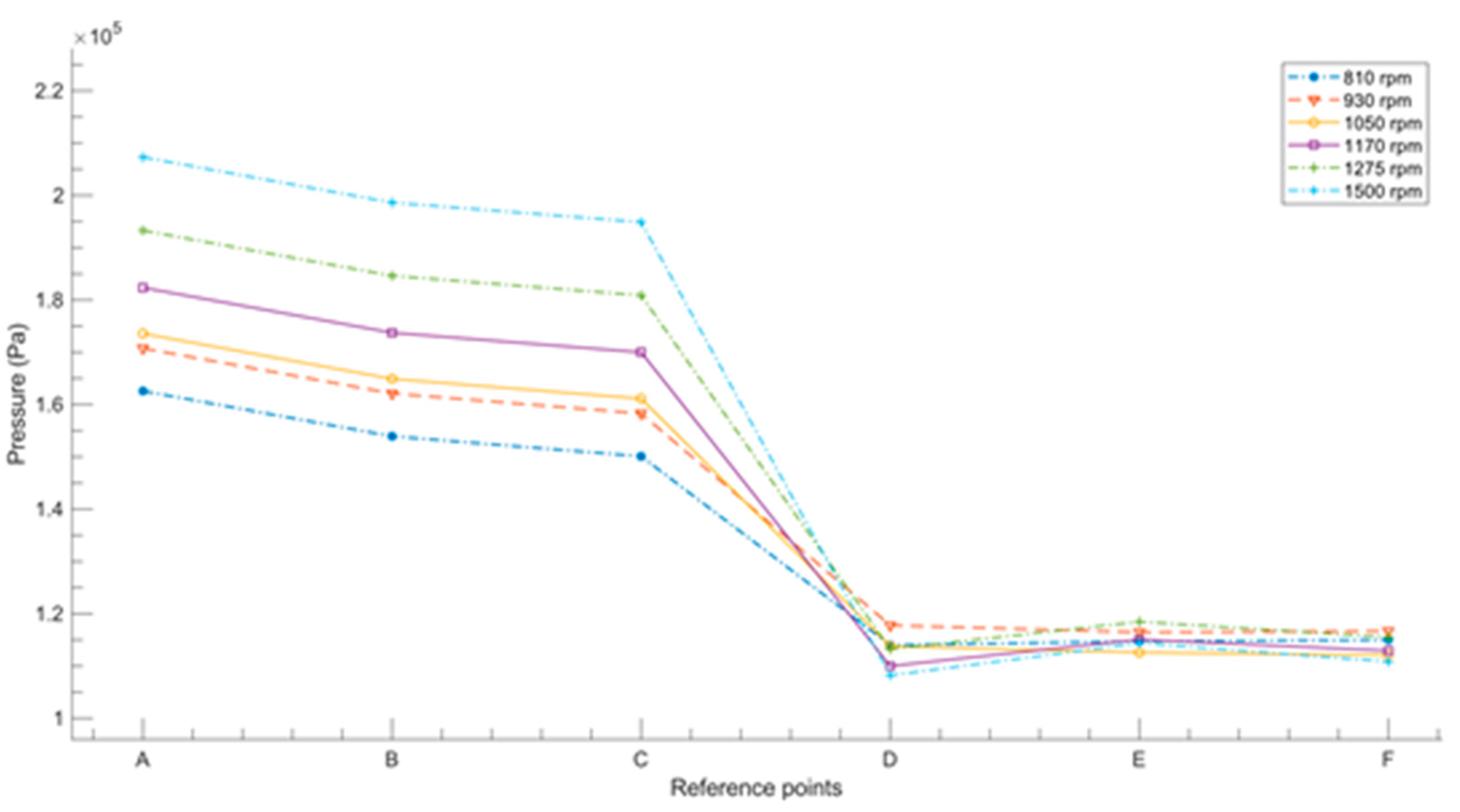
The results of the simulation performed with OpenFOAM in this study, are shown in Figure 5 and Figure 6. As can be seen, the pressure decreases from upstream to downstream, and the lowest pressure value occurs at point D (before the first elbow of the volute outlet) for maximum speed. The error of this simulation concerning the original work varies in ranges from 0.014% up to 14.297% at points A, B, C, and F of the model see Table 5.
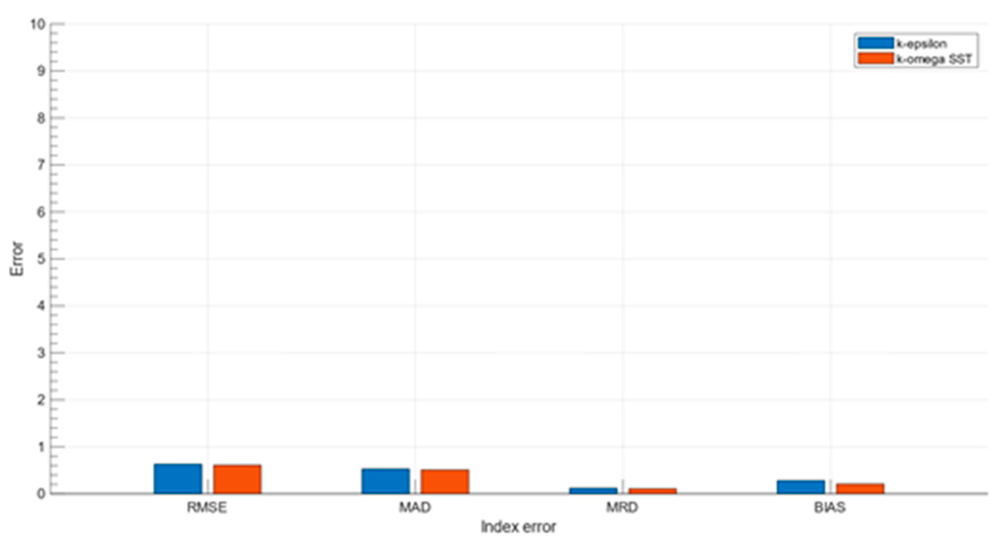
Regarding the calibration of the mathematical simulation with the experimental data, a sensitivity analysis was performed to identify which turbulence model produces the best results. Simulations were executed on the machine's Best Efficient Point (BEP) tested in [51] when operating in turbine mode (QBEP=3.6 l/s) for speeds of 200, 600, 880, 1020, 1200 and 1500 rpm, using the k-e k-w-SST models. The results obtained for both simulations are shown in Table 6. As can be seen, the simulations produced errors of similar magnitude. Still, for the nominal rotational speed of 1020 rpm, the k-w-SST model is the one with the lowest error. An error index analysis was performed to define the turbulence model with which the cases of experimental data, nominal rotational speed curve, and the results of the new expressions [1] will be simulated. Figure 9 shows that in all cases, the k-w-SST model has better performance. So k-w-SST turbulence model was adopted for the rest of the cases.
Once the mathematical model has been validated concerning the results obtained in the numerical modelling and experimental works of [51], the curve of the machine working at nominal speed is contrasted, as seen in Figure 10.
Figure 8. The nominal curve obtained with CFD OpenFoam vs Nominal curve in [51].
Preprints 72124 g008
As can be seen, the simulation performed with OpenFOAM presents satisfactory results, and therefore the model is considered validated.

3.2. Analytical Expressions Validation

3.2.1. Analytical Expressions-New expressions to predict PATs behaviour

Considering that in the case of PATs, the information to select the suitable machines is not known because it is not provided by the manufacturers [55], polynomial expressions have been proposed as a function of semi-empirical methods to estimate the characteristic curves in PATs when the rotational speed is constant [21,55,56,57]. However, considering that flow rates in water systems are variable due to user demand, an optimal energy analysis for PATs cannot be performed if the rotational speed is considered constant. Therefore, strategies have been proposed to maximize energy when the machine works at different rotational speeds, called variable operation strategy (VOS) (19). Plua et al. [1]propose new empirical expressions applying the VOS strategy in water systems for different rotational speeds of 15 different machines and analyzing 87 different curves with 56450 operating points.
Through a mathematical analysis of 10 general expressions (polynomial 6 and 4 potential) considering specific variables as the ratio of rotational speed α, and the ratio Q/QBEP, it was possible to adjust a polynomial function for experimental values of head and efficiency, and a potential function for power. These expressions are observed in equations (3) to (7) and presented the lowest error (30 to 50% compared to other models) in the respective analyses performed where the RMSE, MAD, MRD, and BIAS indices were calculated. Figure 6 of [1] shows a head and efficiency curve comparison between the proposed model, experimental data, and other models.
q = 0 , 1525 ( α Q Q B E P ) + 0 , 1958 ( Q Q B E P ) 2 0 , 0118 ( Q Q B E P ) 0 , 6429 α 2 + 1 , 8489 α 0 , 2241
h = 0 , 31070 ( α Q Q B E P ) + 0 , 3172 ( Q Q B E P ) 2 0 , 0546 ( Q Q B E P ) + 0 , 242 α 2 + 1 , 1708 α 0 , 3426
e = 0 , 8271 ( α Q Q B E P ) 0 , 3187 ( Q Q B E P ) 2 0 , 1758 ( Q Q B E P ) 1 , 035 α 2 + 1 , 1815 α + 0 , 5019
p = α 2 , 4762
q = α 0 , 7439
where
q = Q i Q B E P ; h = H i H B E P ; e = η i η B E P ; p = P i P B E P = q h e

3.2.2. Analytical Expressions Validation

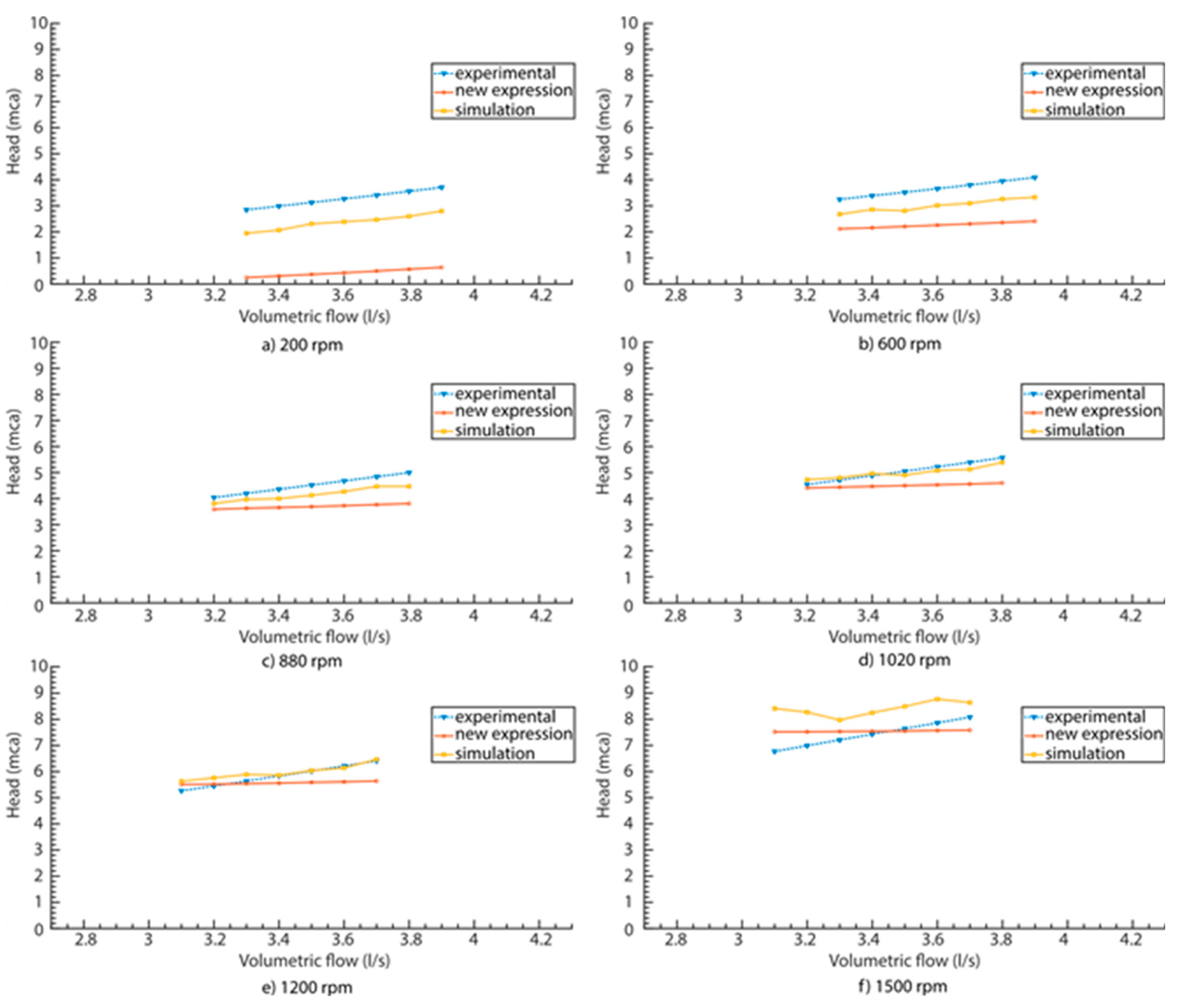
The Head value H for different rotational speeds at points close to the BEP was compared with the experimental Head obtained in [51], the expressions proposed in [1], and the mathematical model. See Figure 11. As can be seen, the relationship between Q and H is increasing in all cases. The predictions made in the numerical simulation with OpenFOAM and with the new expressions present values close to the experimental ones when the operation of the machine approaches the BEP.

3.2.3. Error Analysis

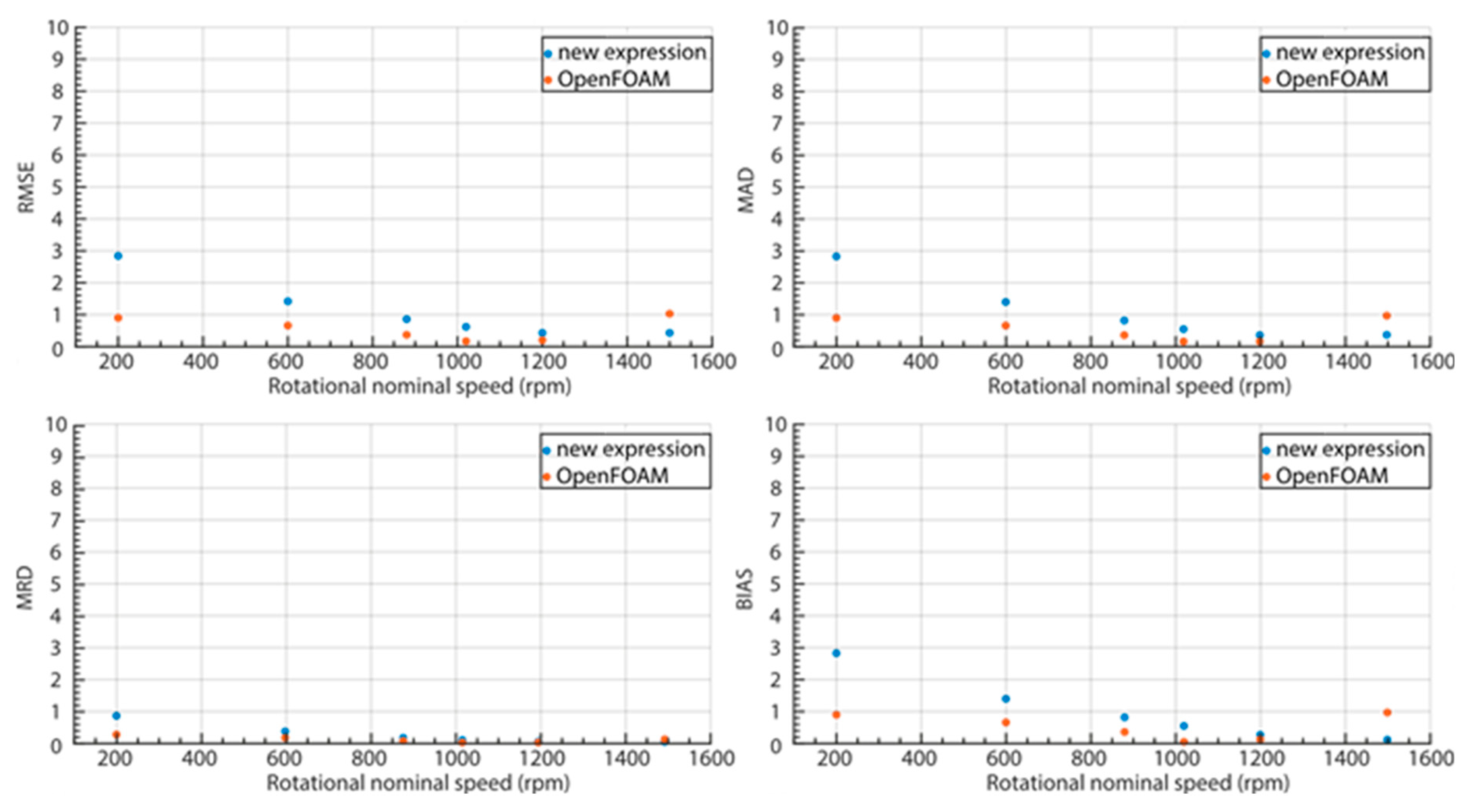
The error rates obtained in the predictions made as a function of the rotational speed are presented in Figure 12. As can be seen, as the conditions approach those of the BEP, the predictions reflect values closer to reality. The range of calculated absolute error for rotational speeds 880 rpm, 1020 rpm,1200 rpm, and 1500 rpm is between 5% to 24%; 2% to 17%, 0% to 12%, and 1% to 24%, respectively.

4. Conclusions

This research proposes to validate as a prediction methodology of Flow (Q) vs Head (H) curves of variable speed PATs, the numerical simulation with OpenFOAM 3D Free Code Package depending on its configuration and working conditions. It also proposes to validate the new expressions submitted by Plua [1]. It was demonstrated that the simulation presents adequate results since the mathematical model and the nominal curve of the Pérez-Sánchez [51] research were calibrated. Furthermore, based on experimental data from a PAT, the Q vs. H curves were calculated through the new expressions [1] as well as with the numerical simulation performed in Openfoam, presenting satisfactory results as the operation point of the work approaches the BEP, since the trend of the generated curves, the slope thereof and the error indices demonstrate acceptable values. However, when moving away from the BEP conditions, the error increases.
The computational domain was divided into four parts: Inlet pipe, rotating part, casing, and outlet pipe. The mesh was created with snappyHexMesh con elements type Hexahedra, Polyhedra, Prism in several 827578. The control conditions imposed on the model were flow and static pressure, and the k-e turbulence model and the k-w-SST model were used, showing that the latter has better results.

Author Contributions

Conceptualization, MPS PALJ; methodology, FP FJSR and MPS software, writing – original draft preparation, VH, FP, MPS; writing – review and editing, PAL-J and MP-S.; visualization MPS PALJ; supervision, MPS and PALJ. All authors have read and agreed to the published version of the manuscript

Funding

Grant PID2020-114781RA-I00 funded by MCIN/AEI/ 10.13039/501100011033.

Institutional Review Board Statement

Not applicable.

Informed Consent Statement

Not applicable.

Data Availability Statement

Not applicable.

Conflicts of Interest

The authors declare no conflict of interest.

References

  1. A Plua, F.; Sánchez-Romero, F.-J.; Hidalgo, V.; López-Jiménez, P.A.; Pérez-Sánchez, M. New Expressions to Apply the Variation Operation Strategy in Engineering Tools Using Pumps Working as Turbines. Mathematics 2021, 9, 860. [Google Scholar] [CrossRef]
  2. M. Farley, “Leakage Management and Control,” Who, pp. 1–98, 2001, [Online]. Available: http://whqlibdoc.who.int/hq/2001/WHO_SDE_WSH_01.1_pp1-98.pdf.
  3. Niu, W.-J.; Feng, Z.-K. Evaluating the performances of several artificial intelligence methods in forecasting daily streamflow time series for sustainable water resources management. Sustain. Cities Soc. 2020, 64, 102562. [Google Scholar] [CrossRef]
  4. Ebrahimi, S.; Riasi, A.; Kandi, A. Selection optimization of variable speed pump as turbine (PAT) for energy recovery and pressure management. Energy Convers. Manag. 2020, 227, 113586. [Google Scholar] [CrossRef]
  5. Orouji, H.; Haddad, O.B.; Fallah-Mehdipour, E.; Mariño, M.A. Modeling of Water Quality Parameters Using Data-Driven Models. J. Environ. Eng. 2013, 139, 947–957. [Google Scholar] [CrossRef]
  6. Vakilifard, N.; Anda, M.; Bahri, P.A.; Ho, G. The role of water-energy nexus in optimising water supply systems – Review of techniques and approaches. Renew. Sustain. Energy Rev. 2018, 82, 1424–1432. [Google Scholar] [CrossRef]
  7. Ferrarese, G.; Malavasi, S. Perspectives of Water Distribution Networks with the GreenValve System. Water 2020, 12, 1579. [Google Scholar] [CrossRef]
  8. Islam, M.S.; Babel, M.S. Economic Analysis of Leakage in the Bangkok Water Distribution System. J. Water Resour. Plan. Manag. 2013, 139, 209–216. [Google Scholar] [CrossRef]
  9. Bibri, S.E.; Krogstie, J. Smart sustainable cities of the future: An extensive interdisciplinary literature review. Sustain. Cities Soc. 2017, 31, 183–212. [Google Scholar] [CrossRef]
  10. Bach, P.M.; Rauch, W.; Mikkelsen, P.S.; McCarthy, D.T.; Deletic, A. A critical review of integrated urban water modelling – Urban drainage and beyond. Environ. Model. Softw. 2014, 54, 88–107. [Google Scholar] [CrossRef]
  11. Raboaca, M.S.; Bizon, N.; Trufin, C.; Enescu, F.M. Efficient and Secure Strategy for Energy Systems of Interconnected Farmers′ Associations to Meet Variable Energy Demand. Mathematics 2020, 8, 2182. [Google Scholar] [CrossRef]
  12. Morani, M.C. , Carravetta, A., D’Ambrosio, C. and Fecarotta, O. A new preliminary model to optimize PATs location in a water distribution network. Environmental Sciences Proceedings 2020, 2, 57. [Google Scholar]
  13. Gupta, A.; Bokde, N.; Marathe, D.; Kulat, K. Leakage Reduction in Water Distribution Systems with Efficient Placement and Control of Pressure Reducing Valves Using Soft Computing Techniques. Eng. Technol. Appl. Sci. Res. 2017, 7, 1528–1534. [Google Scholar] [CrossRef]
  14. Ávila, C.A.M.; Sánchez-Romero, F.-J.; López-Jiménez, P.A.; Pérez-Sánchez, M. Optimization tool to improve the management of the leakages and recovered energy in irrigation water systems. Agric. Water Manag. 2021, 258, 107223. [Google Scholar] [CrossRef]
  15. Ramos, H.; Borga, A. Pumps as turbines: an unconventional solution to energy production. Urban Water 1999, 1, 261–263. [Google Scholar] [CrossRef]
  16. Gallagher, J.; Harris, I.M.; Packwood, A.J.; McNabola, A.; Williams, A.P. A strategic assessment of micro-hydropower in the UK and Irish water industry: Identifying technical and economic constraints. Renew. Energy 2015, 81, 808–815. [Google Scholar] [CrossRef]
  17. Ávila, C.A.M.; Sánchez-Romero, F.-J.; López-Jiménez, P.A.; Pérez-Sánchez, M. Leakage Management and Pipe System Efficiency. Its Influence in the Improvement of the Efficiency Indexes. Water 2021, 13, 1909. [Google Scholar] [CrossRef]
  18. Ávila, C.A.M.; Sánchez-Romero, F.-J.; López-Jiménez, P.A.; Pérez-Sánchez, M. Definition of the Operational Curves by Modification of the Affinity Laws to Improve the Simulation of PATs. Water 2021, 13, 1880. [Google Scholar] [CrossRef]
  19. Ávila, C.A.M.; Sánchez-Romero, F.-J.; López-Jiménez, P.A.; Pérez-Sánchez, M. Optimization tool to improve the management of the leakages and recovered energy in irrigation water systems. Agric. Water Manag. 2021, 258, 107223. [Google Scholar] [CrossRef]
  20. García, I.F.; Novara, D.; Mc Nabola, A. A Model for Selecting the Most Cost-Effective Pressure Control Device for More Sustainable Water Supply Networks. Water 2019, 11, 1297. [Google Scholar] [CrossRef]
  21. Pérez-Sánchez, M.; Sánchez-Romero, F.J.; Ramos, H.M.; López-Jiménez, P.A. Improved Planning of Energy Recovery in Water Systems Using a New Analytic Approach to PAT Performance Curves. Water 2020, 12, 468. [Google Scholar] [CrossRef]
  22. Lee, S.; Pomeroy, C.; Burian, S. Setting Future Water Rates for Sustainability of a Water Distribution System. J. Water Resour. Plan. Manag. 2021, 147, 04020108. [Google Scholar] [CrossRef]
  23. Ahmadi, S.; Saboohi, Y.; Vakili, A. Frameworks, quantitative indicators, characters, and modeling approaches to analysis of energy system resilience: A review. Renew. Sustain. Energy Rev. 2021, 144, 110988. [Google Scholar] [CrossRef]
  24. Stefanizzi, M.; Capurso, T.; Balacco, G.; Binetti, M.; Camporeale, S.M.; Torresi, M. Selection, control and techno-economic feasibility of Pumps as Turbines in Water Distribution Networks. Renew. Energy 2020, 162, 1292–1306. [Google Scholar] [CrossRef]
  25. Renzi, M.; Rudolf, P.; Štefan, D.; Nigro, A.; Rossi, M. Installation of an axial Pump-as-Turbine (PaT) in a wastewater sewer of an oil refinery: A case study. 10th International Conference on Applied Energy (ICAE). LOCATION OF CONFERENCE, COUNTRYDATE OF CONFERENCE; pp. 665–676.
  26. M. Pérez- Sánchez, F. J. M. Pérez- Sánchez, F. J. Sánchez-Romero, H. Ramos M, and P. A. López-Jiménez, Bombas operando como turbinas (PAT) : principios de funcionamiento y selección. Universidad Politécnica de Valencia, 2020.
  27. Binama, M.; Su, W.-T.; Li, X.-B.; Li, F.-C.; Wei, X.-Z.; An, S. Investigation on pump as turbine (PAT) technical aspects for micro hydropower schemes: A state-of-the-art review. Renew. Sustain. Energy Rev. 2017, 79, 148–179. [Google Scholar] [CrossRef]
  28. Novara, D.; Carravetta, A.; McNabola, A.; Ramos, H.M. Cost Model for Pumps as Turbines in Run-of-River and In-Pipe Microhydropower Applications. J. Water Resour. Plan. Manag. 2019, 145, 04019012. [Google Scholar] [CrossRef]
  29. C. P. Thoma, D. C. P. Thoma, D., & Kittredge, “Centrifugal pumps operated under abnormal conditions,” J. Power Sources, vol. 73, no. 1, pp. 881–884, 1931.
  30. P. D. A.J. Stepanoff, Centrifugal and Axial Flow Pumps: Theory, Design, And Application. 1957.
  31. S. Childs, “Convert pumps to turbines and recover HP.,” Hydro Carbon Proces- sing Pet. Refine, vol. 41, pp. 173–174.
  32. Jain, S.V.; Patel, R.N. Investigations on pump running in turbine mode: A review of the state-of-the-art. Renew. Sustain. Energy Rev. 2014, 30, 841–868. [Google Scholar] [CrossRef]
  33. Fecarotta, O.; McNabola, A. Optimal Location of Pump as Turbines (PATs) in Water Distribution Networks to Recover Energy and Reduce Leakage. Water Resour. Manag. 2017, 31, 5043–5059. [Google Scholar] [CrossRef]
  34. Moazeni Faegheh; Khazaei Javad, “Optimal energy management of water-energy networks via optimal placement of pumps-as-turbines and demand response through water storage tanks.,” Appl. Energy, vol. 283, p. 116335, 2021.
  35. Rossi, M.; Renzi, M. A general methodology for performance prediction of pumps-as-turbines using Artificial Neural Networks. Renew. Energy 2018, 128, 265–274. [Google Scholar] [CrossRef]
  36. S. G. Prasad, V. S. G. Prasad, V., Shukla, S. N., & Joshi, “Performance characteristics of pump as turbine. Indian PumpsTitle,” Indian Pumps, vol. 38, no. 4, pp. 5–9, 2006.
  37. Williams, A. Pumps as turbines for low cost micro hydro power. Renew. Energy 1996, 9, 1227–1234. [Google Scholar] [CrossRef]
  38. J. C. Páscoa, F. J. J. C. Páscoa, F. J. Silva, J. S. Pinheiro, and D. J. Martins, “A new approach for predicting PAT-pumps operating point from direct pumping mode characteristics,” 2012.
  39. Rossi, M.; Righetti, M.; Renzi, M. Pump-as-turbine for Energy Recovery Applications: The Case Study of An Aqueduct. Energy Procedia 2016, 101, 1207–1214. [Google Scholar] [CrossRef]
  40. Plua, F.; Hidalgo, V.; Cando, E.; Pérez-Sánchez, M.; López-Jiménez, P. Pumps as Turbines (PATs) by Analysis with CFD Models. Int. J. Adv. Sci. Eng. Inf. Technol. 2022, 12, 1098–1104. [Google Scholar] [CrossRef]
  41. S. Rawal, “Numerical Simulation on a Pump Operating in a turbine mode,” Proc. 23rd Int. users Symp., 2007.
  42. Nautiyal, H.; Kumar, V.; Thakur, A. CFD Analysis on Pumps Working as Turbines. Hydro Nepal: J. Water, Energy Environ. 1970, 6, 35–37. [Google Scholar] [CrossRef]
  43. Páscoa, J.C.; Silva, F.J.; Pinheiro, J.S.; Martins, D.J. Accuracy details in realistic CFD modeling of an industrial centrifugal pump in direct and reverse modes. J. Therm. Sci. 2010, 19, 491–499. [Google Scholar] [CrossRef]
  44. H. Carravetta, A. H. Carravetta, A., Fecarotta, O., & Ramos, “Numerical simulation on Pump As Turbine: mesh reliability and performance concerns.,” in 2011 International Conference on Clean Electrical Power (ICCEP), 2011, pp. 169–174.
  45. Carravetta, A.; Fecarotta, O.; Del Giudice, G.; Ramos, H. Energy Recovery in Water Systems by PATs: A Comparisons among the Different Installation Schemes. Procedia Eng. 2014, 70, 275–284. [Google Scholar] [CrossRef]
  46. F. Pugliese, F. F. Pugliese, F. De Paola, N. Fontana, M. Giugni, G. Marini, and J. F. Francos, “Experimental and numerical investigation of centrifugal Pumps As Turbines,” in Proceedings of the 10th International Conference on Energy Efficiency in Motor Driven System, 2017, pp. 6–7.
  47. Plua, F.; Hidalgo, V.; López-Jiménez, P.A.; Pérez-Sánchez, M. Analysis of Applicability of CFD Numerical Studies Applied to Problem When Pump Working as Turbine. Water 2021, 13, 2134. [Google Scholar] [CrossRef]
  48. Nautiyal, H.; Kumar, V.; Thakur, A. CFD Analysis on Pumps Working as Turbines. Hydro Nepal: J. Water, Energy Environ. 1970, 6, 35–37. [Google Scholar] [CrossRef]
  49. Hidalgo, V.; Velasco, M.; Cando, E.; Valencia, E.; Simbaña, S.; Puga, D.; Mora, C.; Escaler, X. Rotatory 3D structured mesh study using openFOAM to simulate the flow in francis turbine. Mater. Today: Proc. 2022, 49, 142–148. [Google Scholar] [CrossRef]
  50. Hidalgo, V.; Escaler, X.; Valencia, E.; Peng, X.; Erazo, J.; Puga, D.; Luo, X. Scale-Adaptive Simulation of Unsteady Cavitation Around a Naca66 Hydrofoil. Appl. Sci. 2019, 9. [Google Scholar] [CrossRef]
  51. Pérez-Sánchez, M.; Simão, M.; López-Jiménez, P.A.; Ramos, H.M. CFD Analyses and Experiments in a PAT Modeling: Pressure Variation and System Efficiency. Fluids 2017, 2, 51. [Google Scholar] [CrossRef]
  52. Hidalgo, V.; Díaz, C.; Erazo, J.; Simbaña, S.; Márquez, D.; Puga, D.; Velasco, R.; Mafla, C.; Barragán, G.; Parra, C.; et al. Simplified simulation of a small Pelton turbine using OpenFOAM. 2021, 774, 012075. [CrossRef]
  53. File structure of OpenFOAM cases.” https://www.openfoam.com/documentation/user-guide/2-openfoam-cases/2.1-file-structure-of-openfoam-cases (accessed Jan. 11, 2022).
  54. Huang, S.; Wei, Y.; Guo, C.; Kang, W. Numerical Simulation and Performance Prediction of Centrifugal Pump’s Full Flow Field Based on OpenFOAM. Processes 2019, 7, 605. [Google Scholar] [CrossRef]
  55. Fecarotta, O.; Aricò, C.; Carravetta, A.; Martino, R.; Ramos, H.M. Hydropower Potential in Water Distribution Networks: Pressure Control by PATs. Water Resour. Manag. 2014, 29, 699–714. [Google Scholar] [CrossRef]
  56. Novara, D.; McNabola, A. A model for the extrapolation of the characteristic curves of Pumps as Turbines from a datum Best Efficiency Point. Energy Convers. Manag. 2018, 174, 1–7. [Google Scholar] [CrossRef]
  57. Shah, S.R.; Jain, S.V.; Patel, R.N.; Lakhera, V.J. CFD for centrifugal pumps: A review of the state-of-the-art. Procedia Eng. 2013, 51, 715–720. [Google Scholar] [CrossRef]
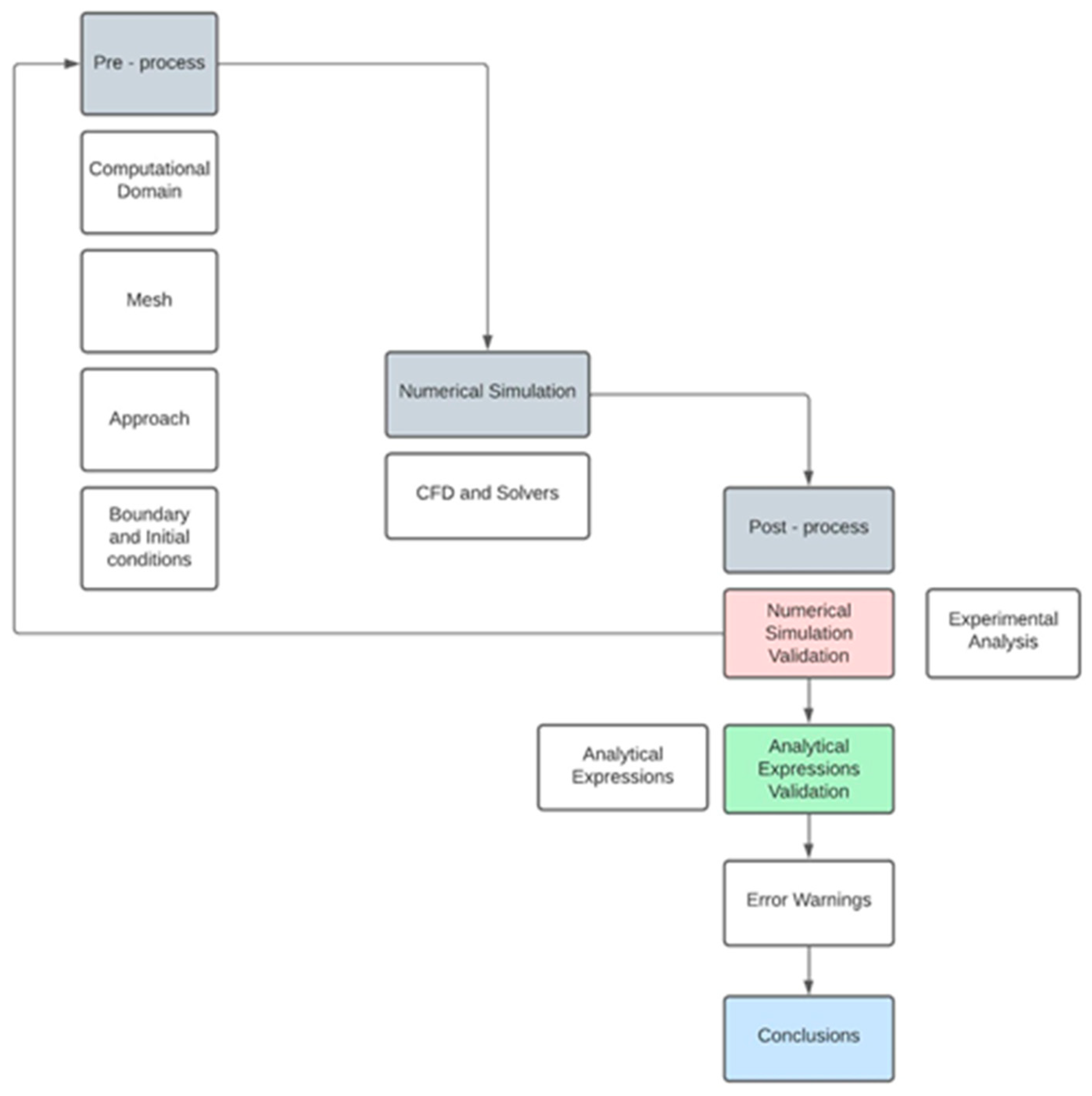
Figure 1. Methodology Flowchart.
Preprints 72124 g001
Figure 2. PAT 3D Model.
Preprints 72124 g002
Figure 3. Domains of the case.
Preprints 72124 g003
Figure 4. Generated mesh.
Preprints 72124 g004
Figure 5. Absolute static pressure contours for Q = 4.50 l/s: (a) N = 810 rpm; (b) N = 930 rpm; (c) N. = 1050 rpm; (d) N = 1170; (e) N = 1275 rpm; (f) N = 1500rpm. .
Preprints 72124 g005
Figure 6. Absolute static pressure vs Referenced sections.
Preprints 72124 g006
Figure 7. Index error analysis for sensitivity analysis.
Preprints 72124 g007
Figure 11. Experimental Head [51] vs Head obtained with new expressions in [1], and CFD OpenFOAM simulation.
Preprints 72124 g009
Figure 12. Error indexes.
Preprints 72124 g010
Table 1. PATs installations in MHP [27].
Location The Capacity of the Plant (kW) Year of Installation
Sainyabulli Province, Laos 2 2008
Thima Kenya 2.2 2001
Mae Wei Village, Thailand 3 2008
West Java, Indonesia 4.5 1992
Kinko village, Tanzania 10 2006
Fazenda Boa Esperanca, Brazil 45 2007
Ambotia Micro-hydro project, India 50 2004
British Columbia, Canada 200 -
Vysni Lhoty, Czech Republic 332 2008
Table 2. Mesh characteristics.
Parameter Value/Characteristic
Element type Hexahedra, Polyhedra, Prism
Number of Elements 827578
Hexaedral 639704
Prism 28238
Polyhedra 159612
Number of Nodes 1203219
Number of Patches 8
Max.Aspect Ratio 14.68619
Min.Surface Area 6.19213 e-09
Min.Volume 1.39587e-11
Max Skewness 12.918596
Table 3. Initial Conditions.
Initial Conditions Value
Turbulent Kinetic Energy ( ) 0.032856(m2/s2)
Turbulent Dissipation Rate ( ) 0.320573(m2/s3)
Specific turbulent Dissipation Rate ( ) 108.4104(s-1)
Turbulent kinematic viscosity (nut) 3.03 x 10⁻⁴(m2/s)
Table 4. Boundary Conditions.
Runner1 Runner RunnerIn Volute Pipe-Inlet Pipe-Outlet Inlet Outlet
Velocity (u-m/s) movingWallVelocity
uniform (0 0 0)
movingWallVelocity
uniform (0 0 0)
movingWallVelocity
uniform (0 0 0)
fixedValue
uniform (0 0 0)
fixedValue
uniform (0 0 0)
fixedValue
uniform (0 0 0)v
flowRateInletVelocity
volumetricFlowRate constant 0.0045
inletOutlet
valueuniform (0 0 0)
Static Pressure
(p-m2/s2)
zeroGradient zeroGradient zeroGradient zeroGradient zeroGradient zeroGradient zeroGradient uniform
115.198(810)
116.694(930)
112.472(1050)
112.909(1170)
115.756(1275)
110.971(1500)
Table 5. Calibration results at points A, B, C and F compared to [51].
%Error
Referenced sections 810 930 1050 1170 1275 1500
A 8,724% 14,297% 8,218% 0,035% 12,881% 14,042%
B 4,455% 10,425% 4,286% 5,324% 9,068% 13,066%
C 5,979% 12,040% 5,643% 3,999% 10,389% 11,936%
F 0,156% 0,014% 0,340% 0,018% 0,199% 0,111%
Table 6. Sensitivity analysis k-e vs k-w-SST.
Experimental Simulation
k-e k-w-SST
n(rpm) H (mca) H (mca) % Error H (mca) % Error
200 3,27 2,28 30,23 2,39 27,00
600 3,66 2,90 20,74 3,02 17,58
880 4,68 4,21 10,10 4,27 8,73
1020 5,22 5,03 3,67 5,08 2,70
1200 6,22 6,21 0,12 6,14 1,30
1500 7,86 8,60 9,35 8,77 11,52
Disclaimer/Publisher’s Note: The statements, opinions and data contained in all publications are solely those of the individual author(s) and contributor(s) and not of MDPI and/or the editor(s). MDPI and/or the editor(s) disclaim responsibility for any injury to people or property resulting from any ideas, methods, instructions or products referred to in the content.
Copyright: This open access article is published under a Creative Commons CC BY 4.0 license, which permit the free download, distribution, and reuse, provided that the author and preprint are cited in any reuse.
Prerpints.org logo

Preprints.org is a free preprint server supported by MDPI in Basel, Switzerland.

Subscribe

© 2024 MDPI (Basel, Switzerland) unless otherwise stated