Submitted:
29 April 2023
Posted:
30 April 2023
Read the latest preprint version here
Abstract
This article derives the closed form solution to finding the roots of a quadratic equation in SU3.
Keywords:
Quaternion
; Quadratic Equation
; Roots
Theorem 1.
The Quadratic Equation , The General Depressed Case
Quadratic Quaternionic Calculator, Closed Form Solution
https://docs.google.com/spreadsheets/d/1X8sKNNuxFq5HLq5qk-93SDVdk6yeh14Xp_OV3bVl2ZI/edit?usp=sharing
Let , which can also be written: We know that there exists a two dimensional basis in the four dimensional space of quaternions that describes the given roots. Namely the bisector of the roots (mistakenly known as the Axis of Symmetry), and the straight line that is between the two roots and the bisector.
We shall define the bisector as as the first vector of the basis.
We now define the locator as
EQ.1 EQ.2 , compelling and EQ.3 Let , therefore EQ.4a EQ.5 EQ.6 EQ.7 EQ.8a EQ.8b If is upon the same great circle as , then the traditional quadratic equation suffices to resolve the roots:
Let , then , where is the Great Circle Function (see page 5).
However, in the general case, it would be exceptionally rare for , so we proceed.
EQ.9a EQ.9b .
EQ.9c . This is the fundamental middle handed form, from which we derive the solution.
EQ.10a Let , such that EQ.11a EQ.12a EQ.13a EQ.14a EQ.15a EQ.16a Let EQ.17a . This is the second fundamental form, the left-handed form.
EQ.9b (a restatement of EQ 9a)
EQ.10b Let , such that , thence:
EQ.11b EQ.12b EQ.13b . This is the third fundamental form, the right-handed form.
However, before we can proceed to resolve the roots of , some general definitions and lemmas are in order.
Definition 1.
Orthogonal Imaginary Bases
EQ.7d and ; furthermore that, and .
and ; furthermore that, and .
and ; furthermore that, and .
If, and only if:
- 1.
- Let ; let ;
- 2.
- 3.
- 4.
- 5.
-
This rigid body rotation of …
- a.
- to
- b.
- to
- c.
- to
which maintains the relative spatial property that .
Definition 2.
A Two-Dimensional Plane in Hypercomplex Space, Absolute Shape.
In Cartesian space, we can define a plane as , however, we cannot do so over the quaternions, there are no real numbers for 72 such that . Rather, we define a plane as a continuum of points that satisfy the below property.
Space and Time Newton and Leibniz https://youtu.be/ZuDkAQvbWj8
EQ.8d Let be the set of all points in the form , where is a purely imaginary unit vector, and is a sum of
all remaining pairwise orthogonal imaginary unit vectors that are orthogonal to , such that there exists an chiral isomorphism from
onto where is the number of hypercomplex dimensions and that all is the set of orthogonal imaginary unit
vectors that this orthogonal basis is Cayley Geodesic, Orientable, Chiral and furthermore Cayley Algebraic (see Appendix A).
Thence such that, .
For the quaternions .
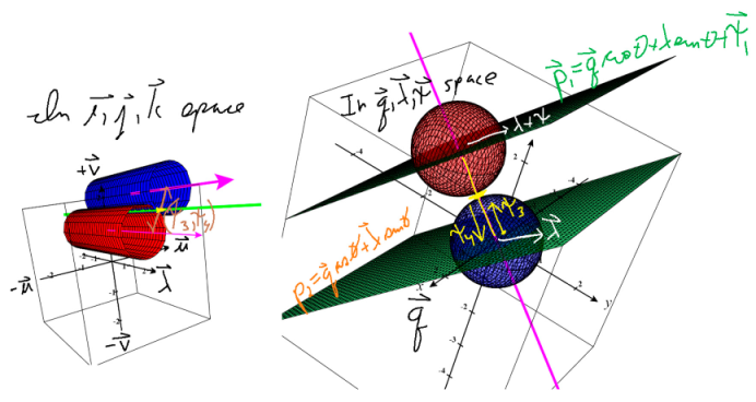
Regardless of the position and facing of different observers, all observers will agree that a collection of objects in (from our perspective) defines a plane from all perspectives. Thus, position and orientation may be relative, but Shape…Shape is Absolute, and Quadratic Equations have a well-defined Shape. In the below image there are three parabolas…but they are all the same, just from three different perspectives.
Definition 3.
Affine Two Dimensional Planes Hypercomplex Space.
EQ.9d Let be the hypercomplex plane such that , EQ.10d Let be the hypercomplex plane such that ,
Corollary 4.
Parallel Two Dimensional Planes Hypercomplex Space.
If and , then and define two parallel two-dimensional subspaces, separated by both , as preference can be given to neither nor and that , such that define the unique line of intersection between two congruent cylinders about and with radii equal to one-half the real number magnitude of in space (which is rotated space, they are the same space, with different bases).
Lemma 5.
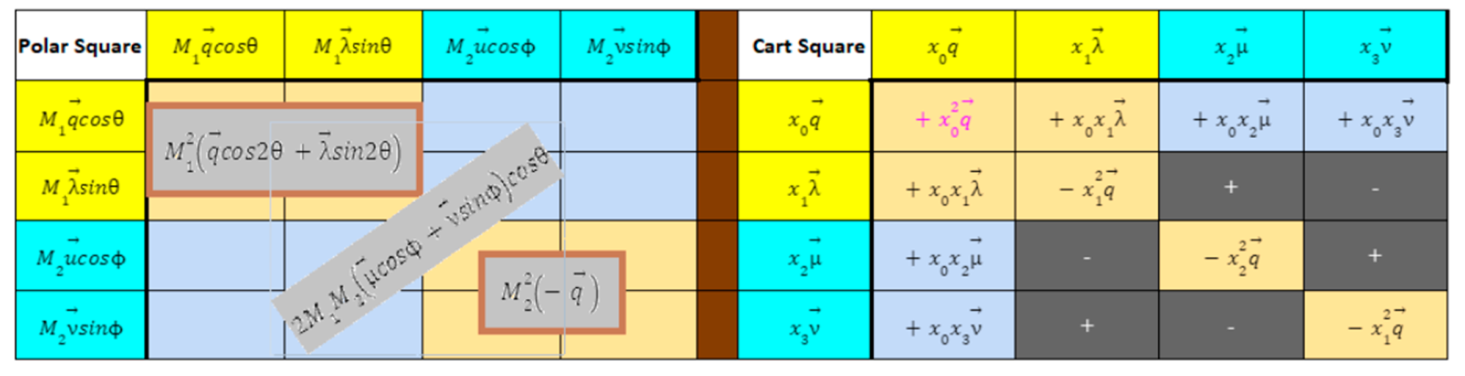
Cayley Multiplication over the General Quaternions, The Square of a Quaternion, Polar and Cartesian Forms.
The rules of are well defined over any imaginary orthogonal basis. Let first separate as .
EQ.1e EQ.2e EQ.3e EQ.4e EQ.5e EQ.6e EQ.7e EQ.8e (this is well known Cartesian form of a quaternionic square)
EQ.9e EQ.10e EQ.11e
Definition 6.
Hypercomplex Chiral Orthogonal Basis Conversion, For the Quaternions
EQ.1f Since , we are only concerned with the imaginary bases, thus:
EQ.2f We already know that:
- 1.
- ;
- 2.
- 3.
- 4.
Let us rename the above as:
EQ.3f EQ.4f EQ.5f Which yields the system of three linear equations:
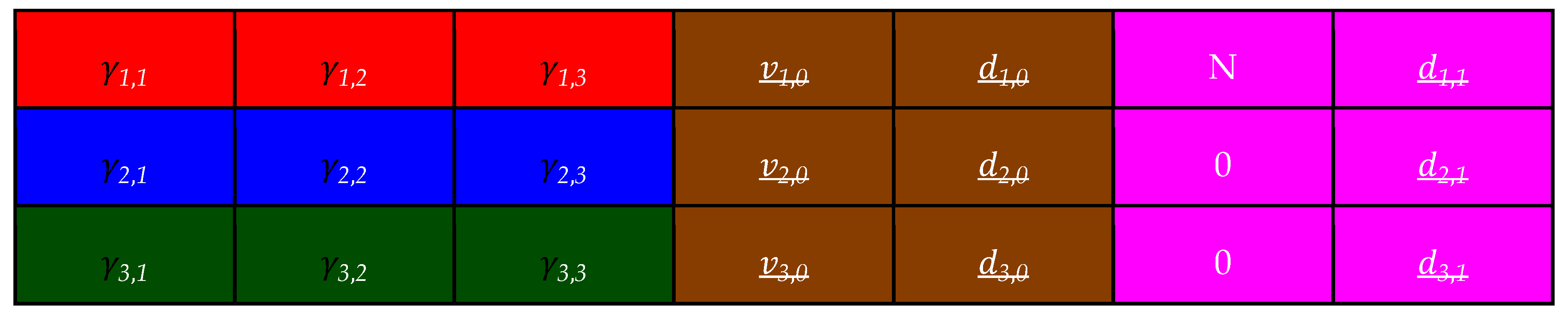
EQ.5f EQ.6f EQ.7f EQ8f Let 𝚪 be a 3x3 real matrix whose pairwise entries are equal to .
EQ9f Let be a 1x3 real column matrix whose entries are and respectively.
EQ10f Let =𝚪-1 , which is also a 1x3 real column matrix
Then are the respective entries of from top to bottom.
Theorem 7.
The Lambda Choice Quaternion Eraser
Statement One when both and are on the same Great Circle of .
Statement Two when both and are not on the same Great Circle and is orthogonal to both and .
Proof.
EQ.1 Let , establishing as the reference frame, compelling the orthogonal basis , then:
EQ.2 Let EQ.3 EQ.4 , since they commute upon the same Great Circle.
EQ.5 EQ.6 EQ.7 , such that is orthogonal to , vanishing and and .
Q.E.D.
Likewise we could establish as the reference frame via: , compelling the orthogonal basis , and the expression will result in vector that is also orthogonal to , vanishing the real part and part of , leaving only and as the remaining dimensions.
Regardless of which reference frame we choose, we know that is orthogonal to both and , and, by definition, anything in the form of is strictly orthogonal to ; however, not everything in form of is strictly orthogonal to .
Also observe that the matrix X = is non-invertible, since any vector with the same imaginary components, but any real component, will evaluate to X . This occurs not only for the hypercomplex numbers, but for the real and complex numbers as well. Consider the following equation:
EQ.8 . Obviously, any real value of will suffice, and any complex value shall also suffice.
EQ.9 . Even though has a non-zero magnitude and is orthogonal to both and , any real or (in respect to ) shall suffice to resolve , hence the inherent invertibility of X = .
However, this does not imply that the appearance of some X = within an equation renders the solution impossible, rather it cannot appear alone, for instance most certainly has a solution for a given and , we would rewrite this as:
EQ.10 .
Hence, the statement also has a solution…two in fact.
However, the most important takeaway is that , meaning the real part of , which is , has no effect; thus, the equation remains equal to , no matter the real part of . Allowing us to reduce the equation to (let and be positive reals):
EQ.11
Theorem 8.
The Right Triangle Theorem
Thence, the expression: geometrically compels to be the hypotenuse of a right triangle, since is orthogonal to both and its square, as both and lay upon the same Great Circle.
Although there exists an entire family of right triangles that share as the hypotenuse, there are only two congruent right triangles within this family that satisfy .
EQ.1 , which is the orthogonal basis in respect to .
EQ.2 EQ.3 is orthogonal to by definition. We shall choose this orthogonality to generate the family of solutions.
EQ.4 is orthogonal to by definition. We discard this orthogonality in favor of the former.
EQ.5 EQ.6 EQ.7 EQ.8 Let EQ.9 Let EQ.10 Let EQ.11 EQ.12 EQ.13 EQ.14 The above relationship provides us with enough information to brute the roots of the quadratic equation by simply comparing every value of the angular argument of against the real number magnitude of error from the return on in a preliminary search, and then converge rapidly upon the roots via bisection.
In fact, it was by empirical observation of the roots (using the above rapidly convergent algorithm) that I was able to resolve the closed form solution. We shall first simplify the quadratic equation further in lieu of those empirical results.
Theorem 9.
The Orthogonal Basis Rotation Theorem; The Relative Frame Theorem.
EQ.1 Let EQ.2a EQ.2b EQ.3 We are able to perform this basis conversion because all we did was rotate about ; hence, preserves the multiplicative relationships expected in the original basis. In fact, there is no preferred frame of reference for the and axes for an Observer on the Great Circle of , only is absolute from the Observer’s perspective. The Observer is free to rotate the axes in any manner that simplifies the existing problem.
Thus, in the equation , the variable establishes , and the variables establishes and . However, we have yet one more simplification to make:
Empirical observation revealed that the equation , always yielded two roots, such that:
EQ.5 , where . That is, when both roots were added together, they left no nor part, and both roots always had the same part. This was true for in excess of 100,000 random trials.
Although empirical observation cannot be used to claim a proof; most certainly assisted in realizing how to derive the closed form solution. Let us briefly examine why the form of would be the solution to our roots.
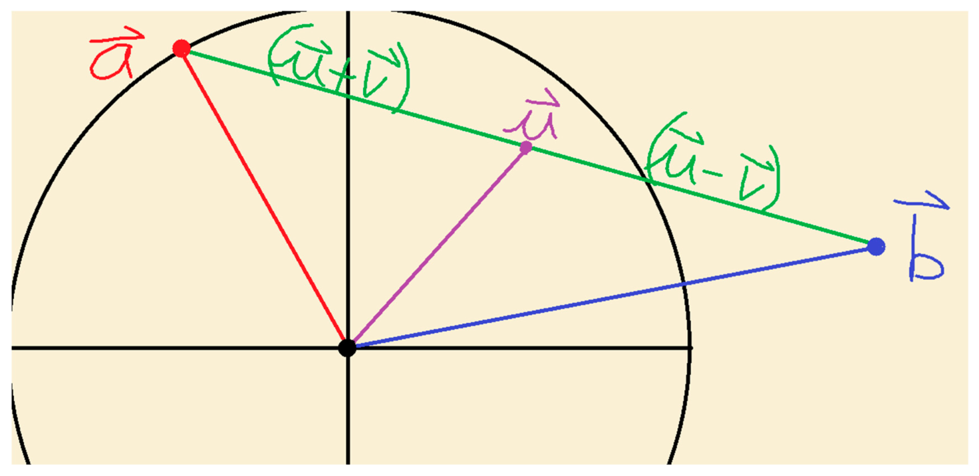
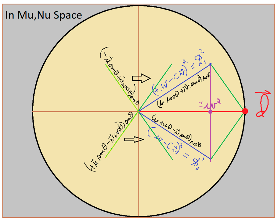
In the image below it shows as the purple vector, located at for some arbitrary chosen theta. It follows that and will form an isosceles triangle, since and will have an equal but opposite reaction with . The green vectors are forced via , since they must be orthogonal to both and . The question of course is which value of in the below diagram produces the correct pair of magnitudes for the blue and green legs that have a sum square of one when they interact with the magnitude of .
Theorem 10.
The Fully Depressed Case of the Quadratic Equation
We now combine Theorems 14 and 15 to yield the fully depressed case of the quadratic equation. We shall remove the real part of and rotate the orthogonal axes in respect to and then divide by the orthogonal magnitude of … and we shall simply write as EQ.1a , where is in respect to .
EQ.1b EQ.1c , where is the initial orthogonal basis in respect to .
EQ.2a Let EQ.2b Let EQ.2c Let EQ.2d Let EQ.2e Let EQ.3a EQ.3b EQ.3c (Lambda Choice Quaternion Eraser)
EQ.4a EQ.4b EQ.4c EQ.4d
Lemma 11.
The Mu Part and Nu Part Equivalence.
EQ.5a EQ.5b EQ.5c EQ.6a EQ.6b EQ.6c EQ.7a EQ.7b EQ.7c .
Lemma 12.
The Real Part and Nu Part Equivalence.
EQ.1a EQ.1b EQ.2a EQ.2b EQ.2c EQ.2d EQ.3a EQ.3b EQ.3c EQ.3d
Lemma 13.
The Lambda Part Identity
EQ.1 EQ.2 EQ.3
Lemma 14.
The Real Part Identity
EQ.1 EQ.2 EQ.3 EQ.4 EQ.5 EQ.6 EQ.7 EQ.8 EQ.9 EQ.10 EQ.11 EQ.12 EQ.13 EQ.14 EQ.15 EQ.16 EQ.17 EQ.17a EQ.17b EQ.17c EQ.17d
Definition 15.
Cardano’s Theorem: The Real Cubic Identity of the Nu Part
We now use the Cardano Method to depress the Cubic of the Nu Part.
EQ.1 EQ.2 EQ.3 EQ.4 EQ.5 Completing Cardano’s depression of the Cubic. We now implement Vieta’s Substitution:
Definition 16.
Vieta’s Theorem: The Resolution of the Nu Part.
EQ.1 EQ.2 EQ.3 EQ.4 EQ.5 EQ.6 EQ.7 , either sign of the square root shall suffice.
EQ.8 EQ.9 We now use the identities from to yield and .
EQ.10 EQ.11 EQ.12 Of course, we have a serious dilemma. Which of the three real roots do we accept for ? Which sign of the above squares do we choose in unison? Only the polar form of solution will elucidate which root of to accept, and then how to produce and .
Theorem 17.
The Offset Circle Theorem
For the moment, let us suppose we know which cubic root to select as , then we now examine the following relationship: . This equation informs us that the coordinate lays upon a circle, with a radius of , offset from the origin by .
Let , then the Law of Cosines reveals that:
EQ.1 EQ.2 EQ.3 , upholding the Law of Sines.
We now examine the relationship .
EQ.4 EQ.5 EQ.6 EQ.7 EQ.8 EQ.9 EQ.10 , which leads to a nasty degree six equation with 6 pairs of conjugate solutions for .
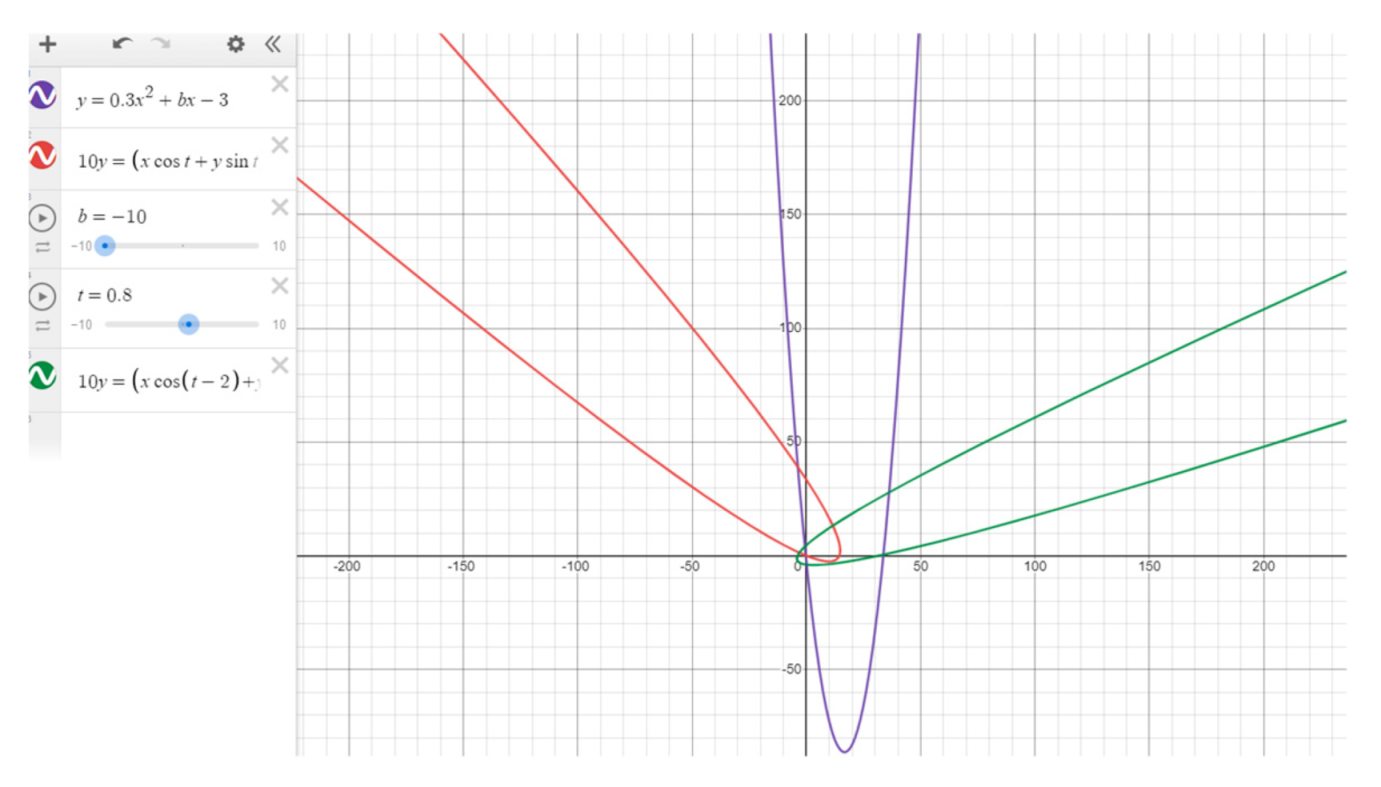
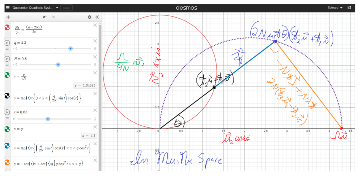
Before we proceed, the below image is the geometric appearance of the question at hand in space.
In the following url link, is Omega, N is N, and t is theta: https://www.desmos.com/calculator/q2bfcbs7wq
However, when we yield the roots of the cubic to produce we can solve for theta without any of the hassle that the polar form introduces.
EQ.11 EQ.12 EQ.13 EQ.14 EQ.15 . We know to take the positive root, since the coordinate resides in the first quadrant, since both magnitude variables, and , are positive by definition, forcing the red circle (in the above image) in the upper two quadrants. We also both angles for the Arcsine function. This is not because we cannot resolve the ambiguity; rather, both solutions fulfill simultaneously. Hence:
EQ.16 ; yielding the empirically observed form: , where has no part.
With both values of theta known, we simply use the identities above to yield EQ.17a EQ.17b . Q.E.D.
Theorem 18.
The Six Root Equivalence Theorem
At this moment in the paper, there is no known method to determine which of the three cubic roots to choose for . However, a simple guess and check on the resulting coordinates suffices, since the coordinate must have a magnitude of . That is, given:
EQ.1 , when does:
EQ.2 EQ.3 EQ.4 EQ.5 EQ.5 EQ.6 EQ.7 EQ.8 EQ.9 Which informs us that all three cubic roots suffice, and thus a Quadratic Equation over the Quaternions has three pairs of roots that conjugate over the 307 axis, since all resultant Arcsine values yield the reflexive property . Thus there exists six solutions to a Quaternionic Quadratic.
However, only one of the three real roots with return a Real Value of Theta for , while the other two roots shall return imaginary values for theta.
That does not mean however that we discard these solutions, since any resulting imaginary unit is equal to , but rather that it introduces non-real coefficients against the vector components, and culmination of these coefficients in the form of recombine when multiplied against the and vector components to yield the exact same value of as the real coefficients that resulted from the root whose was also real.
That is, all three Arcsine arguments of produce the same vector after recombination.
Q.E.D.
Theorem 19.
The Closed Form Solution for a General Quadratic Equation for the Quaternions.
We now combine all of the steps to solve original query:
EQ.1 EQ.2 Let EQ.3 EQ.4 EQ.5 EQ.6 Let , therefore EQ.7 EQ.8 Let EQ.9 EQ.10 EQ.11 EQ.12 EQ.13 EQ.14 329 EQ.15 EQ.16 Let 𝚪 be a 3x3 real matrix whose pairwise entries are equal to .
EQ.17 Let be a 1x3 real column matrix whose entries are and respectively.
EQ.18 Let be a 1x3 real column matrix whose entries are and respectively.
EQ.19 Let 𝐕 =𝚪 , which is also a 1x3 real column matrix, let it the results be named . is our first primary variable.
EQ.20 Let =𝚪 , which is also a 1x3 real column matrix, let it the results be named We do not require the inverse Gamma Matrix for this process.
𝚪 Gamma Matrix Matrix Matrix 𝚪 = Matrix 𝚪 = Matrix
EQ.21 EQ.22 EQ.23 EQ.24 EQ.25 EQ.26 EQ.27 EQ.28 EQ.29 EQ.30 EQ.31 EQ.32 EQ.33 EQ.34 EQ.35 EQ.36 EQ.37 EQ.38 EQ.39 EQ.40 EQ.41 EQ.42 EQ.43 , either sign of the square root shall suffice, and any cube root will suffice.
EQ.44 EQ.45 . All roots will be real.
EQ.46 . If is a complex number, then is the imaginary unit.
The complex arguments of can be used, substituting for and then wielding these complex coefficients against the and vector components of . However, to avoid confusion, it is most practical check all three roots of and just select the real argument of EQ.47 EQ.48 The above two equations are the roots in the proper orthogonal basis of , however we must now convert back to .
EQ.49 EQ.50 EQ.51 EQ.52 EQ.53 EQ.54 EQ.55 EQ.56 EQ.57 EQ.58 Recall that and therefore and that .
EQ.59 EQ.60 EQ.61 EQ.62 EQ.63 The above two equations satisfy the original query , proving that all Quadratic Equations over the Quaternions adhere to the same closed form solution.
Q.E.D.
Statements and Declarations
I have nothing to declare.
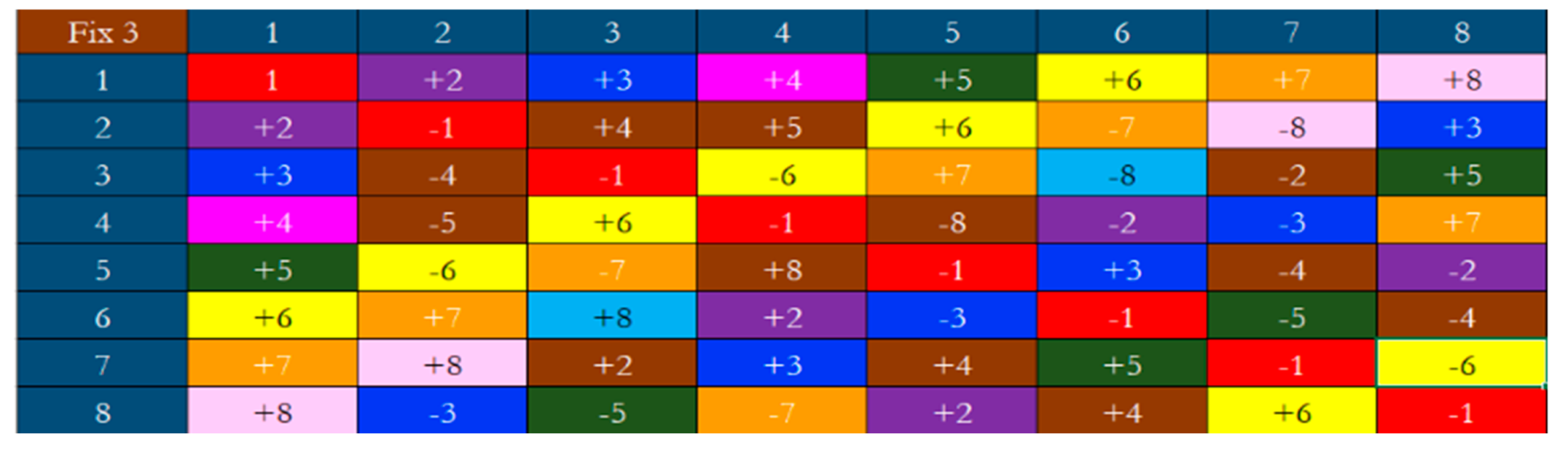
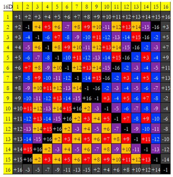
Appendix A. Overview of Cayley Geodesicity, Orientability, Chirality, Algebraicity
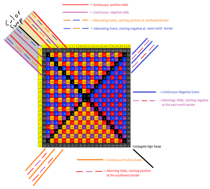
In Volume Two, when we move beyond the Quaternions, we shall give this topic proper treatment. For now, a summary of the definitions of Geodesicity, Orientability, Chirality and Algebracity shall suffice. Below are three Cayley Tables of four, six and twenty-two dimensional hypercomplex spaces that satisfy these four properties. We shall not address odd dimensional spaces until Volume Three.
1 . A Cayley Table is said to be Geodesic if each orthogonal imaginary unit vector appears once, and only once, in each row and column.
2 . A Cayley Table is said to be Orietnable if the square of each imaginary unit vector is equal to and the square of .
3 . A Cayley Table is said to be Chiral if it is both Geodesic and Chiral, and the resulting sign of each Cayley product is the opposite of its transposed product for the Even Dimensional Spaces.
4 . A Cayley Table is said to be Algebraic if it is Geodesic, Oreitnable and Chiral, and that the resulting product signs adhere to uniform pattern over the product grid that allow one to calculate all roots of -unity for all hypercomplex vectors in that space.
We shall cover the specific pattern of sign placement that admits Algebracity in Volume Two. For now, see if you can discern the pattern of positive 91 and negative sign placement in the 22D table. The first dimension, is in the below table.
Algebraic Icosidgions
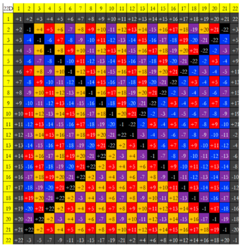
In all of the below tables, the dimension 1 is equal to .
Algebraic Hexonions
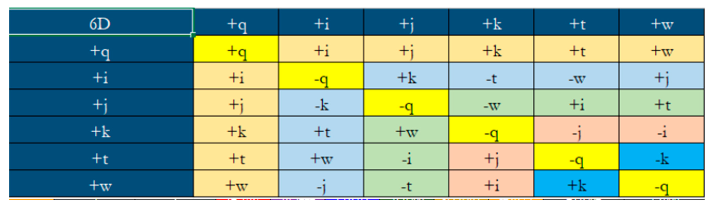
Algebraic Octonions
Algebraic Sedenions
I do not feign to know why the below paradigm works, I only know that it works (via copious brute force experiments). Only the below layout of dimension and sign placement allows one to take the Mth root of N unity (see Appendix B) for the Even Hypercomplex Complex Numbers and locate the roots of a quadratic equation.
Appendix B. The M-th Root of N-Unity for Class of Algebraic Hypercomplex Numbers of Even Dimensions, The Great Circle Theorem
Assuming that we are in a Hypercomplex Space that is Cayley Algebraic, then let be the function that returns the principal root unity for .
EQ.11d Let be the observation vector.
EQ.12d Let be the set of pairwise orthogonal imaginary unit vectors, and must be odd, such that is even.
EQ.13d Let such that EQ.14d Let , which is the real number magnitude of the imaginary part of .
EQ.15d Let , which is the real number magnitude of .
EQ.16d Let , compelling to be a unit vector.
EQ.17d Let , giving us the ratio between the magnitudes of the real part and the imaginary part.
EQ.18d Let , that is, the four-quadrant arccotagent of .
EQ.19d EQ.20d
Appendix B.2. Corollary: The Square Root of a Quaternion, The Well Defined Positive and Negative Square Roots
For a quaternion , the square root is given by:
EQ.21d
Appendix C. The Quadratic Equation , The Trivial Case of Symmetric Roots, For All Hypercomplex Dimensions
EQ.1e can be readily solved for even if and are not on the same Great Circle.
EQ.2e Let , such that EQ.3e EQ.4e EQ.5e EQ.6e EQ.7e EQ.8e EQ.9e Q.E.D
It is our goal to transform the earlier equation, , into the Symmetric Case via a series of additional substitutions.
The Symmetric Case occurs when .
References
- https://mathworld.wolfram.com/VietasSubstitution.html.
- https://www.math.ucdavis.edu/~kkreith/tutorials/sample.lesson/cardano.html.
Disclaimer/Publisher’s Note: The statements, opinions and data contained in all publications are solely those of the individual author(s) and contributor(s) and not of MDPI and/or the editor(s). MDPI and/or the editor(s) disclaim responsibility for any injury to people or property resulting from any ideas, methods, instructions or products referred to in the content. |
© 2023 by the authors. Licensee MDPI, Basel, Switzerland. This article is an open access article distributed under the terms and conditions of the Creative Commons Attribution (CC BY) license (http://creativecommons.org/licenses/by/4.0/).
Copyright: This open access article is published under a Creative Commons CC BY 4.0 license, which permit the free download, distribution, and reuse, provided that the author and preprint are cited in any reuse.


