Preprint
Article

Data-Assisted Training of a Physics-Informed Neural Network to Predict the Reynolds-Averaged Turbulent Flow Field around a Stalled Airfoil under Variable Angles of Attack

Altmetrics

Downloads

477

Views

287

Comments

0

  + These authors contributed equally to this work.

This version is not peer-reviewed

Submitted:

28 April 2023

Posted:

30 April 2023

You are already at the latest version

Alerts
Abstract
Physics-informed neural networks are a promising method to yield surrogate models of flow fields. We present a metamodeling technique for variable geometries based on physics-informed neural networks. The method was applied to the DU99W350 airfoil at a Reynolds number of 1×10⁵. The model predicted the Reynolds-averaged velocity and pressure field around the airfoil for arbitrary angles of attack between 10.0° and 17.5°. The model was trained with data from CFD simulations for a limited set of angles of attack. Additionally, satisfaction of the a priori known boundary conditions as well as the Reynolds-averaged Navier-Stokes equations were trained. A sensitivity analysis concerning the Reynolds number, the amount and distribution of training data, and the turbulence model was conducted showing the superiority of the pseudo-Reynolds stress method and the demand of labeled training data in the domain. The trained network was capable of predicting the developing flow separation on the suction surface and exhibited excellent agreement with CFD results even in the proximity to the wall for interpolations as well as extrapolations from the labeled data set.
Keywords: 
Subject: Computer Science and Mathematics  -   Artificial Intelligence and Machine Learning

1. Introduction

Surrogate models play an important role in product development, optimization problems, real time processing, or sub modelling. In many cases, surrogate models are required to replace CFD simulations due to their high computational costs. A surrogate model can be built via a fit to sample points that can either be simulated or measured. Prevalent models comprise linear regression, Bayesian models, random forests, and neural networks (NN), among others [1].
According to the approximation theorem of Pinkus, a single hidden layer NN with enough neurons can approximate any function and its derivatives [2]. This feature makes NN suitable for surrogate modeling as it avoids limitations in regression accuracy to complex functions that are related to other surrogate methods, such as linear regression. Consequently, several investigations show a superiority of NN when compared to other regression models [3,4,5]. A vast variety of different architectures and algorithms of NN have been developed and applied, comprising feedforward NN, recurrent NN, convolutional NN, reinforcement learning, or generative adversarial networks, among others [6]. A drawback of NNs is the need for large high-quality datasets in the training process [7].
Recently, physics-informed neural networks (PINN) have become a focus of research activities. A PINN is a NN that is trained to respect given laws of physics, typically partial differential equations (PDE), as well as boundary conditions (BC). In the training process, PINNs create sample data by solving the PDE under the given BC. Hence, a lack of simulation or measurement data can be compensated. Since flow measurements and CFD simulations are often time consuming and expensive, the use of PINNs could improve and shorten the surrogate modelling process.
The concept of PINN has first been described by Lagaris et al. [8] who showed the applicability of PINNs to solve several ordinary differential equations (ODEs), coupled ODEs and PDEs. Raissi et al. [9,10,11] solved the Burgers equation, the Schrödinger equation, and the Allen-Cahn equation with a PINN for time dependent one-dimensional problems. The results exhibited excellent agreement between the PINN and the exact solution. The publications presented above demonstrated the suitability of PINNs to solve PDEs.
PINNs were also applied to the field of fluid dynamics to solve the Navier-Stokes (NS) equations. Here, investigations cover the application of feedforward NNs to two- and three dimensional problems [12], near wall flows [13], thermal flows [14,15], cavitation flows [16], reconstruction of incomplete data [17,18], boundary condition enforcement and adaptive activation functions [19], convolutional PINNs [20,21], and different fomulations of the NS equations [22], among others.
In most publications PINNs were used to predict flow fields for Reynolds numbers below 300 [12,14,19,22,23]. However, many technical problems are subject to high Reynolds numbers and corresponding turbulent flows. Turbulent flows result in highly complex flow fields in both space, and time. Hence, solving the Naver-Stokes equations with a PINN for highly turbulent flows can be a challenging task. As for many applications only stationary information is required, PINNs predicting the Reynolds-averaged Navier-Stokes (RANS) equations incorporating a turbulence model are suitable. A first approach has been done by Hennigh et al. [24] who applied the mixing length turbulence model. Eivazi et al. [25] trained a PINN to statisfy the RANS equations without a transport-equation-based model to predict a turbulent boundary layer, the high Reynolds flow in a sub domain on an airfoil, as well as a flow over a periodic hill. Xu et al. [26] used a similar approach and trained a PINN to predict the turbulent viscosity without any imposed equation. They trained the model to CFD data and used it to explore missing flow data inside of a finite area downstream of a backward-facing step. Pioch et al. [27] applied the mixing length model, the k- ω model, an equation-free pseudo-Reynolds stress model and an equation-free ν t model to a backward facing step flow. A favourable agreement with data from a direct numerical simulation was found when three or five lines of labeled training data were used.
In the research presented above, PINNs were trained to predict a two- or three-dimensional solution for a single geometry. Wandel et al. presented a convolutional PINN that takes the vector potential as an input. The model was trained with different 3D shapes, such as boxes, cylinders, or spinning balls. They reported plausible flow fields for geometries not contained in the training dataset, such as a fish or multiple boxes [28]. Hennigh et al. presented the NVIDIA SimNet framework that can read standard tesselation language (stl) files and comes with the zero-equation mixing length turbulence model. They applied the framework on the NVSwitch with parameterized geometry and used a modified Fourier feature PINN to find the optimal parameter configuration [24]. Arthurs and King presented an active learning algorithm and trained a PINN to predict the flow and pressure field in a tube for two shape parameters and reported low errors [29]. These investigations demonstrate the general suitability of PINNs as surrogate models for flows around variable geometries. To further assess the capabilities and limitations of PINNs as multidimensional surrogate models of variable geometries, investigations of complex flows at high Reynolds numbers are needed.
In this work, we contribute to the question how multidimensional surrogate models of Reynolds-averaged flows could be generated using a PINN and how accurately the flow field is predicted. As an example, we present a PINN-based surrogate model of the DU99W350 airfoil at a high Reynolds number of 1 × 10 5 using the Python library DeepXDE [30]. The model takes the two-dimensional coordinates as well as the angle of attack as input parameters and predicts the mean pressure and velocity fields around the airfoil. To investigate the applicability of PINNs to complex fluid dynamics, the model was designed to predict the developing flow separation on the suction surface. In the training process, the RANS equations were solved. We tested the standard k- ω model by Wilcox [31] and a pseudo-Reynolds stress turbulence modeling approach [25,27]. We evaluate the accuracy of the model when compared to CFD simulations and further discuss the limitations and potential improvements of the presented PINN methodology. The scope of this work was to investigate the capability of a simple feed-forward network architecture to serve as a surrogate model of a complex Reynolds-averaged flow around a parameterized geometry at an elevated Reynolds number.

2. Set up and reference flow field

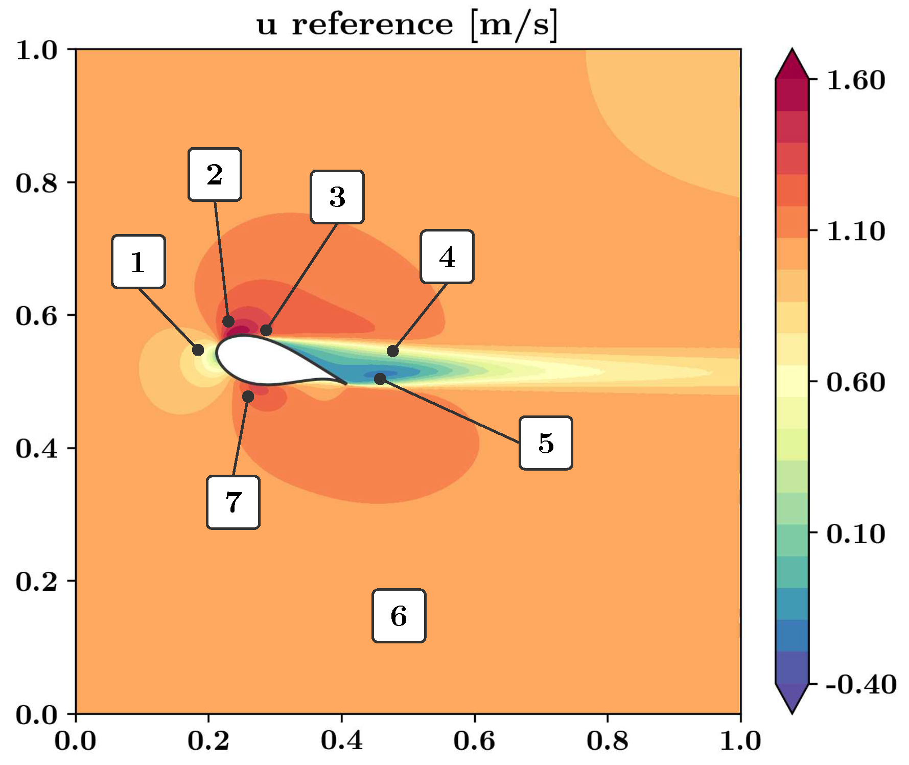
As an application example, we used the DU99W350 airfoil positioned inside a channel. This airfoil is employed for blades of wind turbines such as the NREL 5 MW turbine [32]. We have chosen this example as the presented surrogate modeling technique could be employed in real time steering algorithms as well as aerodynamic optimization problems. This example is further suited to investigate the prediction quality of realistic flow fields. The channel had a height and a width of 1 m and the chord length c of the airfoil was 0.2 m. For variations of the AoA, the airfoil was rotated around the leading edge. Figure 1 schematically illustrates the geometry as well as the simulated mean flow field around the airfoil for an angle of attack of 15.0 . As indicated in the figure, the flow features a stagnation point at the leading edge of the airfoil, a boundary layer around the airfoil, multiple regions of high velocity gradients, and a separated flow on the suction surface.

3. Methodology

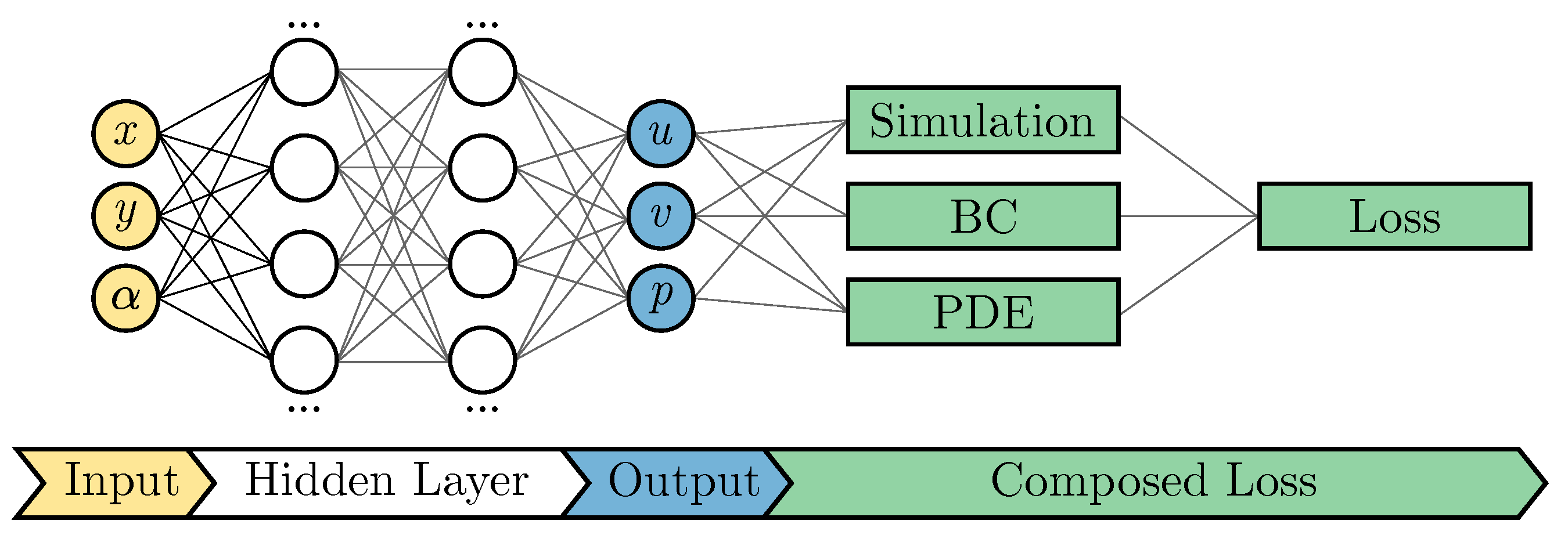
To yield the multidimensional surrogate model, a feedforward NN was trained to predict the Reynolds-averaged velocity and pressure field. The input layer of the NN consisted of three neurons that represent the three input dimensions coordinates x, y, and angle of attack (AoA) α . In case the neural network is trained without any turbulence model, the output layer comprises three neurons and displays the Reynolds-averaged predictions of u, v, and p. The PINN then reads:
N N θ x y α = u v p
where θ are the trainable parameters (weights and biases) of the NN. Figure 2 shows the corresponding architecture. As sketched, the output of the NN is fed into three different losses that build a so-called composed loss function.
In the composed loss function, losses for boundary conditions, simulated training values, and a system of partial differential equations (PDEs) were added. The composed loss function L reads:
L ( θ ) = L b ( θ ) + L d ( θ ) + L e ( θ )
with the adjustable network weights and biases θ , the loss on the boundary conditions L b , the loss for the training data L d , and the loss for the partial differential equations L e . The individual loss terms were calculated using the mean squared error:
L b = 1 n b n = 1 N b | U b n U ˜ b n | 2
L d = 1 n d n = 1 N d | U d n U ˜ d n | 2
L e = 1 n e k = 1 3 n = 1 N e | ε k n | 2
where N b , N d , and N e represent the number of points for which the boundary conditions, labeled training data, and PDEs are trained. U b n = [ u b n , v b n ] and U d n = [ u d n , v d n , p d n ] are the given data for point n on the boundaries and for the labeled data coordinates, respectively. U ˜ b n and U ˜ d n represent the output of the PINN at the corresponding points and ε k n is the residual of the kth equation at point n.
In this work, the continuity equation and the two-dimensional Reynolds-averaged Navier-Stokes equations for an incompressible fluid were used as PDEs. The corresponding residuals read:
k = 1 = u i ¯ x i
k = 2 , 3 = u j ¯ u i ¯ x j + u j u i x j ¯ + 1 ρ p ¯ x i ν 2 u i ¯ x j x j
with Reynolds-averaged velocities and pressure u i ¯ , u j ¯ , and p ¯ , constant density ρ , and constant kinematic viscosity ν . The RANS equations contain the Reynolds stress terms:
τ i j x j = u j u i x j ¯
Here, τ i j represents the Reynolds stresses. For traditional turbulence modeling as applied in computational fluid dynamics (CFD), the Reynolds stresses are estimated using the Boussinesq hypothesis:
τ i j = u i u j ¯ = ν t ( u i ¯ x j + u j ¯ x i ) 2 3 k δ i j
where k is the turbulent kinetic energy, δ i j is the Kronecker delta, and ν t is the turbulent viscosity. This approach is based on the gradient diffusion hypothesis which states that the turbulent transport is aligned with the negative gradient of the mean flow. The isotropic turbulent viscosity ν t then serves as a diffusion coefficient, supposing an analogy between viscous stresses and turbulent stresses.
In this work, we considered two different turbulence-modeling approaches. The first model is the standard k- ω model of Wilcox [31]. This model is frequently applied for CFD calculations. For the k- ω model, the turbulent viscosity is calculated using:
ν t = k ω
with the specific dissipation rate ω . The 2D stationary equations for k and ω read:
u j ¯ k x j = τ i j u i ¯ x j β * k ω + x j ( ν + σ * ν t ) k x j
u j ¯ ω x j = α k ω τ i j u i ¯ x j β ω 2 + x j ( ν + σ ν t ) ω x j
with β * = 9 / 100 , σ * = σ = 0 . 5 , α = 5 / 9 , β = 3 / 40 , as recommended by Wilcox [31]. For the composed loss function, the transport equations for k and ω are to be included in the system of PDEs. The corresponding PINN reads:
N N θ x y α = u v p k ω
The second considered model is a pseudo-Reynolds stress model as applied by Eivazi et al. [25] and Pioch et al. [27]. For this model, the Reynolds stress terms are calculated without any specific modeling using only two pseudo-turbulent velocity fluctuations, u p and v p :
τ i j x j = u j p u i p x j
Using this approach, in the training process the NN is penalized to learn an averaged flow field as well as pseudo-Reynolds variables that together satisfy the RANS equations. The corresponding PINN reads:
N N θ x y α = u v p u p v p
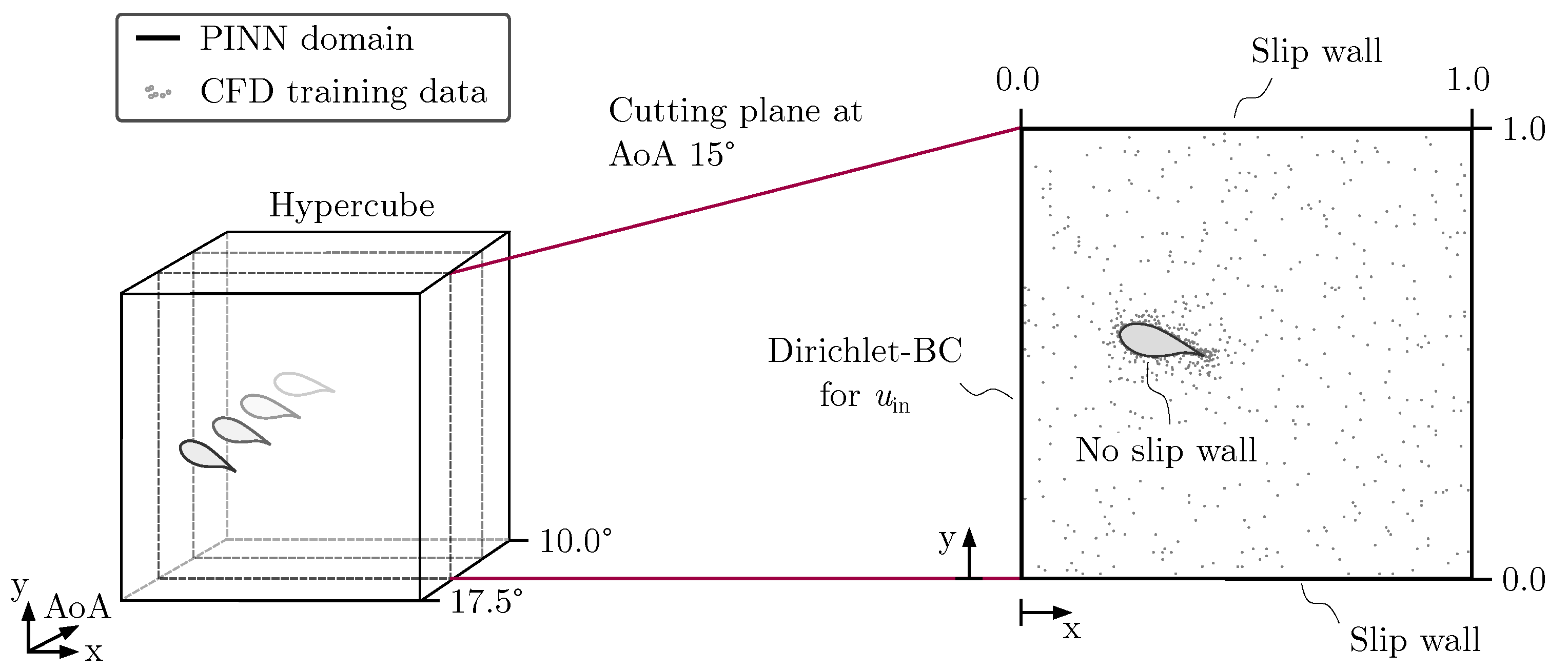
To calculate the losses associated with the boundary conditions, a slip wall condition was defined for the upper and lower channel walls. For the airfoil surface, we used a no slip wall condition. At the left boundary of the channel, we deployed a velocity inlet boundary condition. No pressure outlet condition was defined.
Setup and training of the multidimensional PINN was done with a custom Python code using the tensorflow-based library DeepXDE [30]. The model was trained with the described RANS equations and boundary conditions as well as simulation data. We used a PointSetBC to train the labeled reference data and anchor points to train the PDEs.
To define the training points inside the multidimensional training domain, the coordinates of two different CFD grids were used. The grids were generated with for different AoA. To obtain the labeled training data, two-dimensional simulations were carried out with Comsol Multiphysics 5.6 on a hybrid mesh consisting of unstructured triangular finite elements and layers of quadrilateral elements to account for the boundary layer. The mesh featured 15 inflation layers with a growth rate of 1.1, a maximal base size of 0.01 m with a maximal growth rate of 1.08, as well as a grid refinement on the airfoil surface with a maximum cell size of 0.002 m. The trial functions were 2nd order accurate. Further, a hybrid wall function, the k- ω turbulence model and a convergence limit of 10 5 were defined. The maximal y + value was 2.9. The pressure values were downscaled by a factor of 10 3 . To train the PINN, a batch of random data points was drawn from the complete labeled data set ahead of the training process. The coordinates for the training of the PDEs were derived from a coarser grid without any further selection. Some illustrations concerning the training coordinates are given in the Appendix. The advantage of this method is the concentration of training points in important regions such as the boundary layer. The training of the PDEs as well as the boundary conditions was conducted for AoA of 10.0°, 12.5°, 15.0°, and 17.5°. Labeled training data were considered for AoA of 10.0 and 15.0 only.
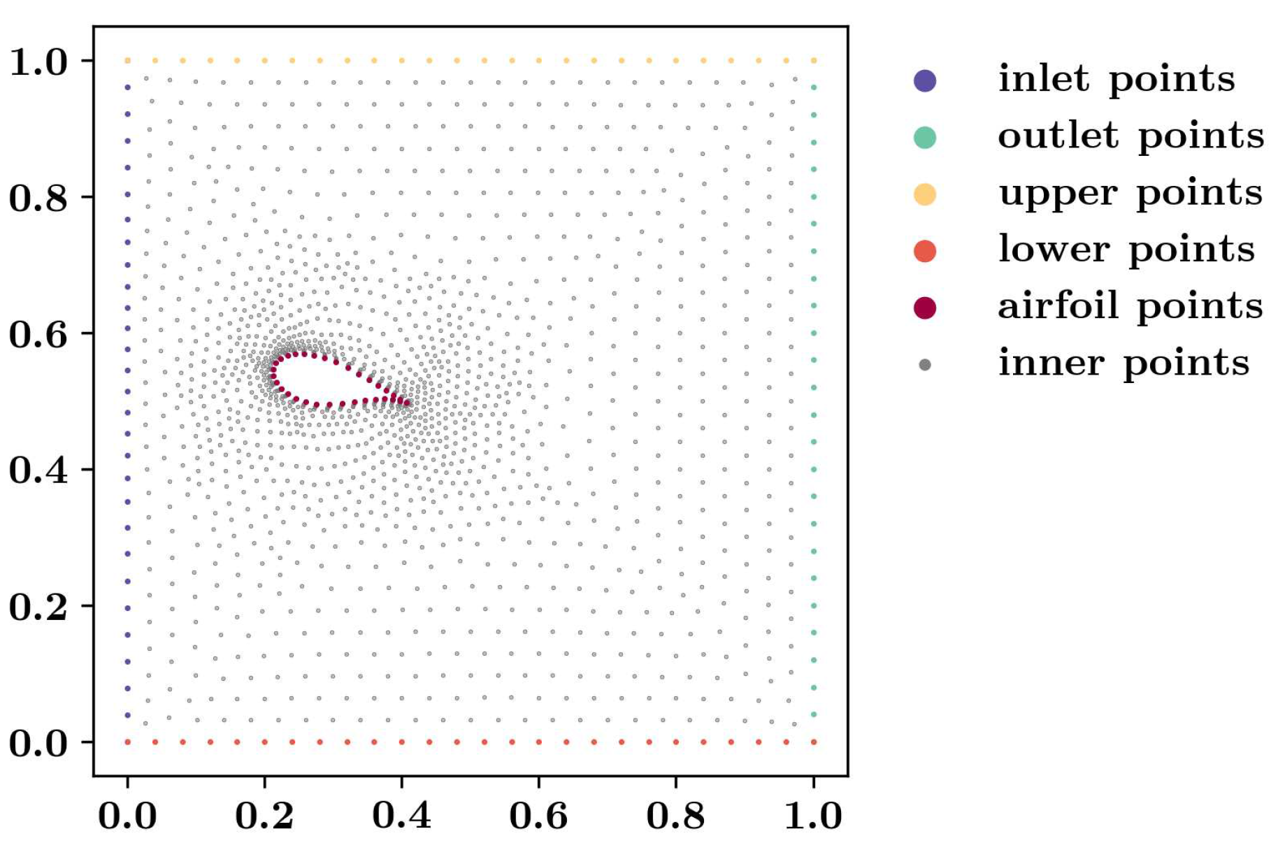
Figure 3 illustrates the applied boundary conditions as well as the considered training data. As seen, the training domain was built by a multidimensional hypercube and the training of the PINN was conducted at discrete AoA which represent slices of the hypercube. This procedure facilitated the generation of training coordinates for specific AoA using a CFD meshing algorithm. The PINN could then be trained on these coordinates using the PointSet boundary conditions for the labeled data and the anchor points for the PDEs. This method was applied as the automatic generation of appropriately positioned training coordinates for n-dimensional problems is challenging. In this case, definition of the n-dimensional geometry as well as a suitable training point coordinate generator were necessary. The method applied here allows, in contrast, for point generation using available CFD meshers discretizing two- or three-dimensional geometries which can be obtained using conventional computer aided design (CAD) software. If we assume that a three-dimensional geometry then was to be trained for one parameter in the fourth dimension, such as AoA, then the training points could be generated for the geometry at discrete AoA.
For the training of the neural network, the loss terms were weighted using:
L = λ b L b + λ d L d + λ e L e
with λ b , λ d , and λ e as constant weight factors for boundary conditions, labeled training data, and PDEs, respectively. In the training procedure, the weights and biases θ of the NN were adjusted using the optimizers Adam and L-BFGS to minimize the weighted composed loss function. The model was trained for 30,000 epochs using the Adam optimizer. Afterwards, the model was further trained with the L-BFGS optimizer under the predefined default settings. In the Appendix, a supplementary illustration concerning the corresponding losses for PDEs, BCs, and labeled data is given. Table 1 lists the relevant training parameters.
We trained a NN consisting of five hidden layers with 128 neurons each. The training was repeated ten times to account for the random initialization of the weights and biases. For the further evaluation, the model with the lowest normalized mean squared error (NMSE) was selected.

4. Sensitivity analyses

In this section, results of several preliminary sensitivity analyses are presented. For these investigations, we limited the training to an AoA of 15.0°. The number of training points n d , n b + n d , and n e were 800, 1600, and 1558, respectively. The scope of this section was to identify important training settings and to evaluate the accuracy of the corresponding predictions. Here, we present evaluations of the Reynolds number and the corresponding scaling method, the amount and distribution of training data, and a comparison between the k- ω model and the pseudo-Reynolds stress model.
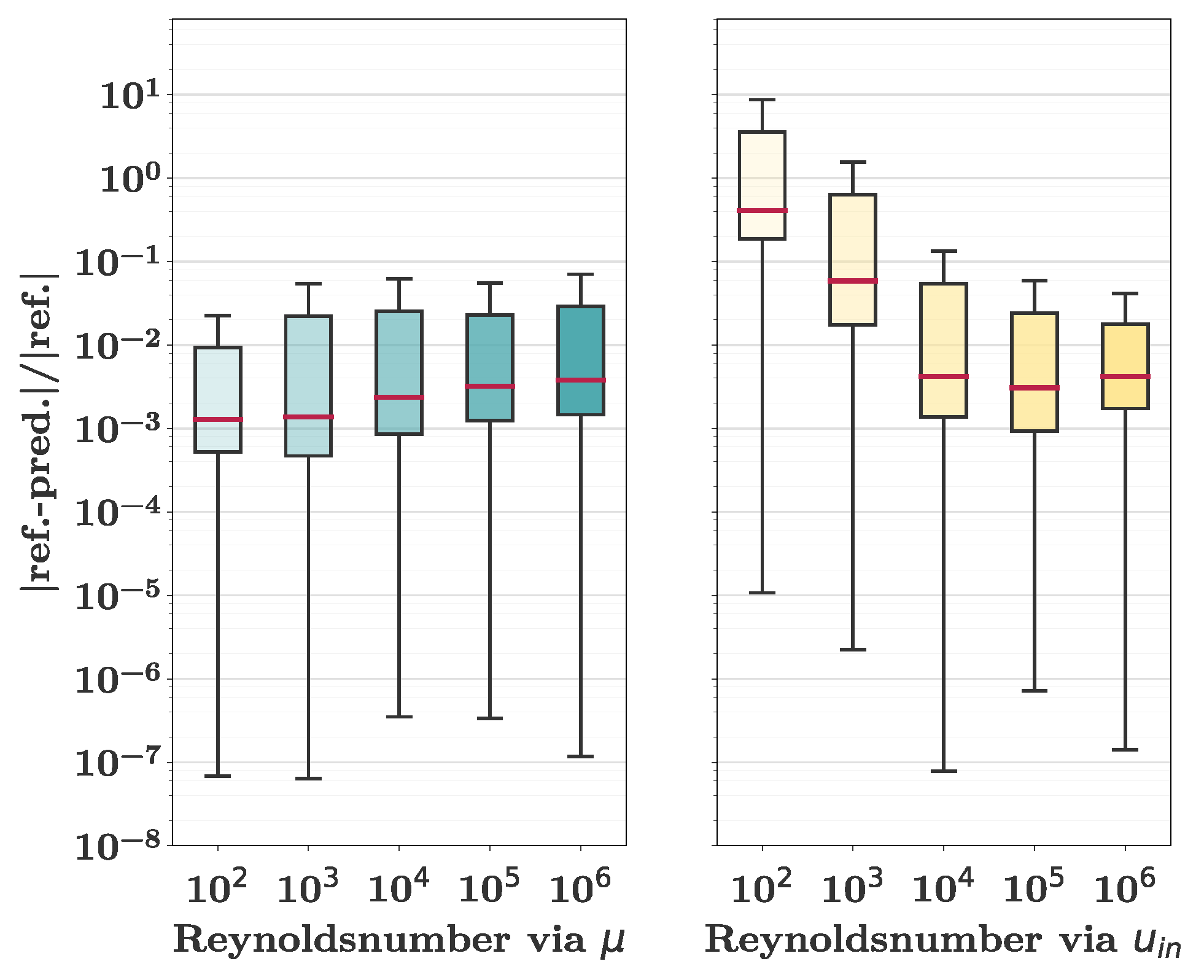
For the investigations concerning the Reynolds numbers, we tested the accuracy of the training for Re c { 10 2 , 10 3 , 10 4 , 10 5 , 10 6 } . These Reynolds numbers were obtained following two different procedures. For the first approach, a fluid with a density ρ of 1000 kg / m 3 and a dynamic viscosity μ of 0.001 kgm 1 s 1 was defined. The inlet velocity u was then varied between and 0.0005 m/s and 5 m/s. For the second approach, the inlet velocity was set to 1 m/s and the viscosity was varied between 0.2 kgm 1 s 1 and 0.0002 kgm 1 s 1 . The results of this analysis are shown in Figure 4. The training runs with different inlet velocities exhibited severe deviations from the reference solutions for lower Reynolds numbers. The training using a variable viscosity showed excellent agreement between the predictions and the reference data over the whole range of Reynolds numbers. However, the absolute error grew non-linearly with the associated Reynolds number. This finding is in agreement with the results of Sun et al. [19] who, however, covered lower Reynolds numbers. The results demonstrate the necessity for an appropriate scaling of the investigated problem. For a successful training, input and output dimensions of the neural net needed to match. This was also found by Laubscher and Rousseau [14] who trained the non-dimensional Navier-Stokes equations.
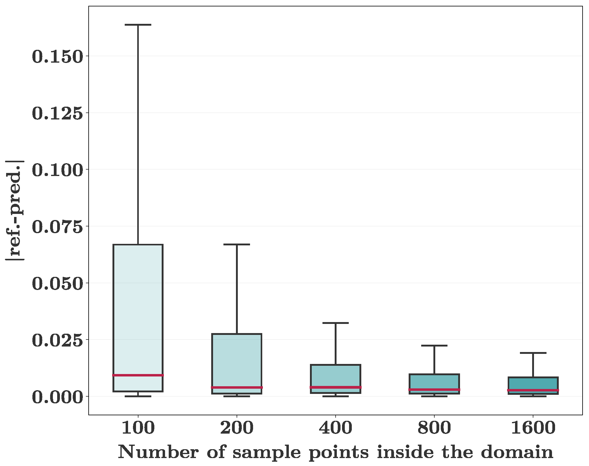
For the investigation concerning the amount of labeled training data, we used different numbers n d of training points: n d { 100 , 200 , 400 , 800 , 1600 } . The total number of points n b + n d on boundaries and labeled data was consequently set to n b + n d { 200 , 400 , 800 , 1600 , 3200 } . Figure 5 exhibits the corresponding results. As illustrated, the prediction accuracy positively correlated with the amount of training data. This finding emphasizes the requirement of introducing enough labeled training data for successfully training the PINN and is in agreement with the observations of Pioch et al. [27]. As n d > 800 , the reduction of the error stagnated. In the subsequent analysis, n d was, consequently, set to 800 for every trained AoA that was supplied with labeled training data.
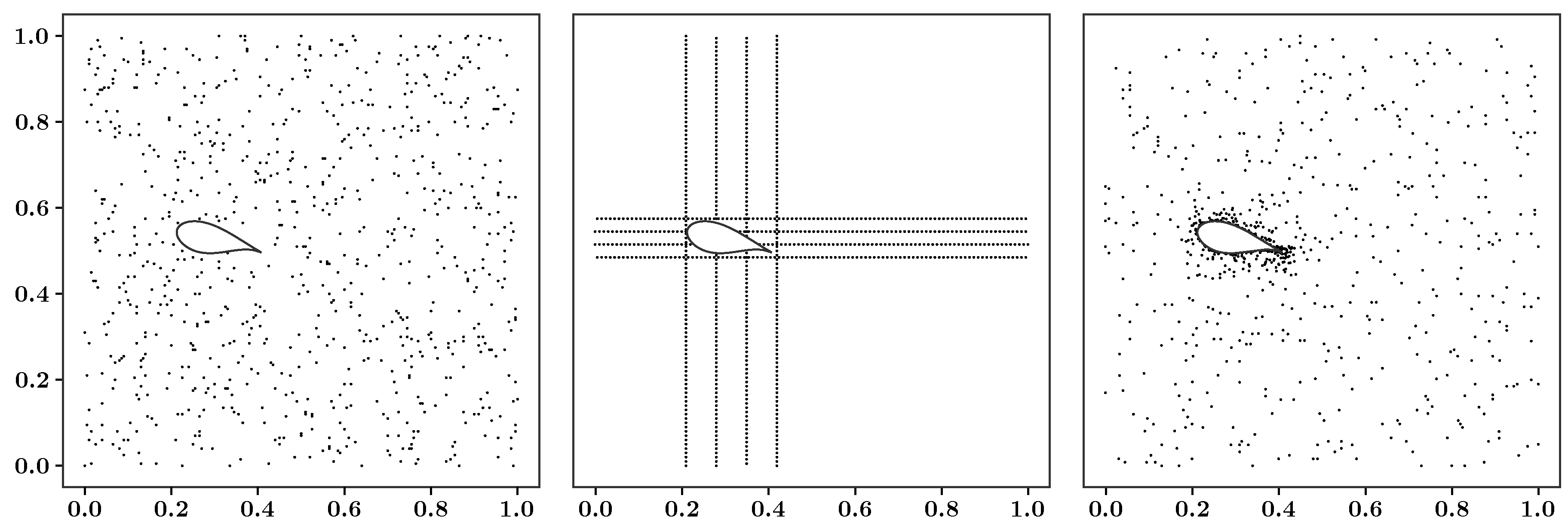
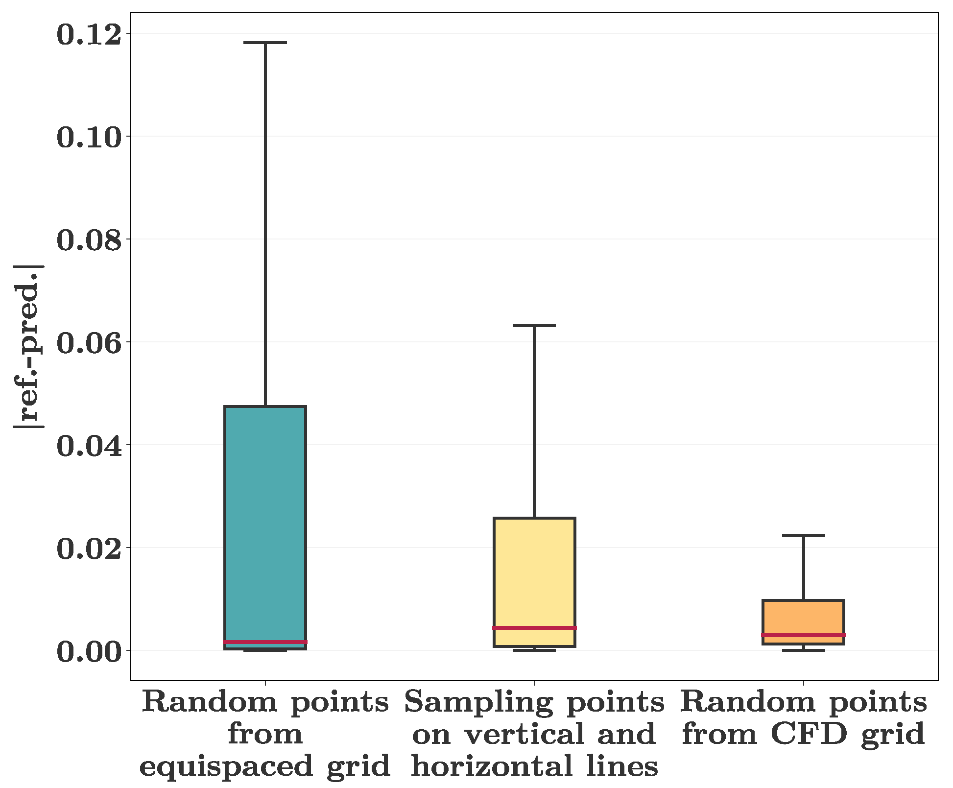
In a third step, a comparison between three different labeled training data sampling strategies was performed. For this analysis, the prediction accuracy obtained using 800 randomly selected coordinates from a CFD grid as well as from a uniform grid with a spacing of 0.005 m was compared with a distribution of training data along several vertical and horizontal lines. The vertical lines were positioned at x { 0 . 21 , 0 . 28 , 0 . 35 , 0 . 42 } and the horizontal lines were positioned at y { 0 . 485 , 0 . 515 , 0 . 545 , 0 . 575 } . The number of points n d on the lines was 767. Some illustrations concerning the training coordinates are given in the Appendix. Figure 6 shows the results of this analysis. From the results it is evident that the randomly selected training data drawn from a CFD grid outperformed the other approaches.
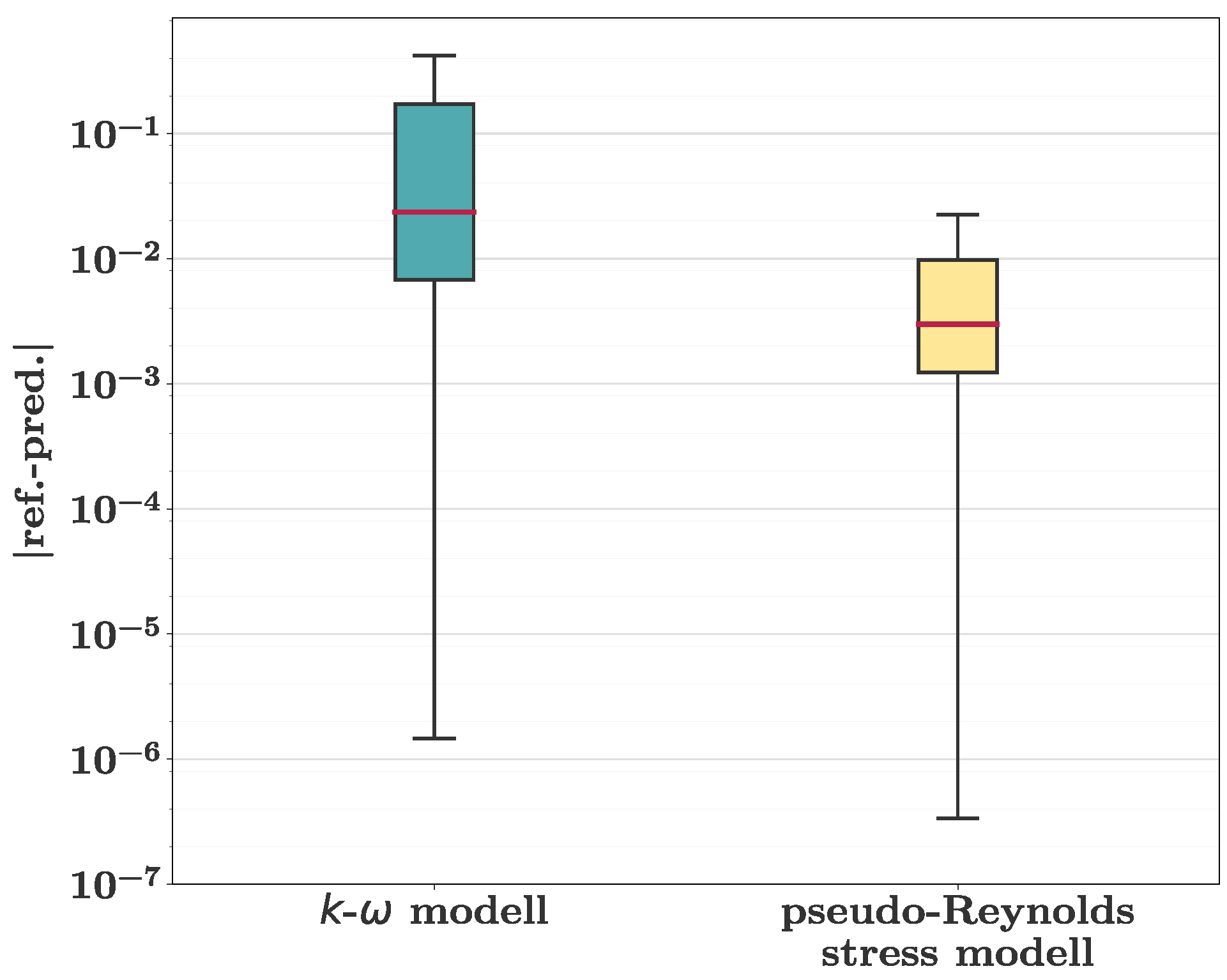
To assess the effect of different turbulence models, we compared the standard k- ω model and the pseudo-Reynolds stress model, as described above. Figure 7 illustrates the obtained predictions. The pseudo-Reynolds stress model exhibited a favorable agreement with the reference CFD data while the predictions obtained with the k- ω model were subject to significant deviations. This result demonstrates the importance of an appropriate turbulence modeling approach. A potential explanation for the different outcomes of the two models is given in Section 5.6 and Section 5.7.
As the described investigations revealed the superiority of a scaling using a variable viscosity, a random distribution of data points drawn from a CFD grid, the pseudo-Reynolds stress model, as well as the requirement to set at least 800 points of labeled training data per AoA into the domain, the training of the multidimensional surrogate model for variable angles of attack was set up accordingly.
We have further tested the application of a Fourier-feature NN as well as different weighting factors λ b , λ d , and λ r . However, these investigations did not show significant effects on improving the performance and, hence, are not covered here.

5. Results and discussion

In this section, the results of the multidimensional training for the PINN predicting the two-dimensional flow field for variable AoA are presented. We first show the results at an AoA of 15.0°. At this angle, labeled training data were provided during the training. Subsequently, the capability of the PINN to interpolate and to extrapolate is evaluated for AoA of 12.5° and 17.5°. In the following, we discuss the accuracy of the results as well as challenges and potential improvements for future work.

5.1. Prediction at an AoA of 15.0°

Figure 8 presents the results of the PINN in comparison with the reference data for an AoA of 15.0°. The prediction contained all relevant flow features and the flow separation as well as the high speed regions were depicted accurately. The mean deviations of the axial velocity between PINN and CFD results were 3 . 8 × 10 3 m/s which represents 0.38% of the reference inlet velocity. The highest errors could be observed at the leading edge of the airfoil, in the stagnation point region, and in the separated shear layer.

5.2. Interpolation at an AoA of 12.5°

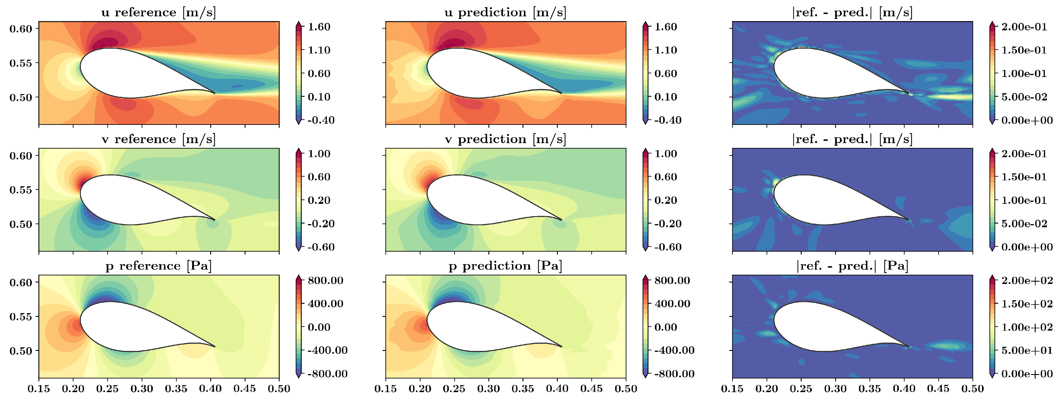
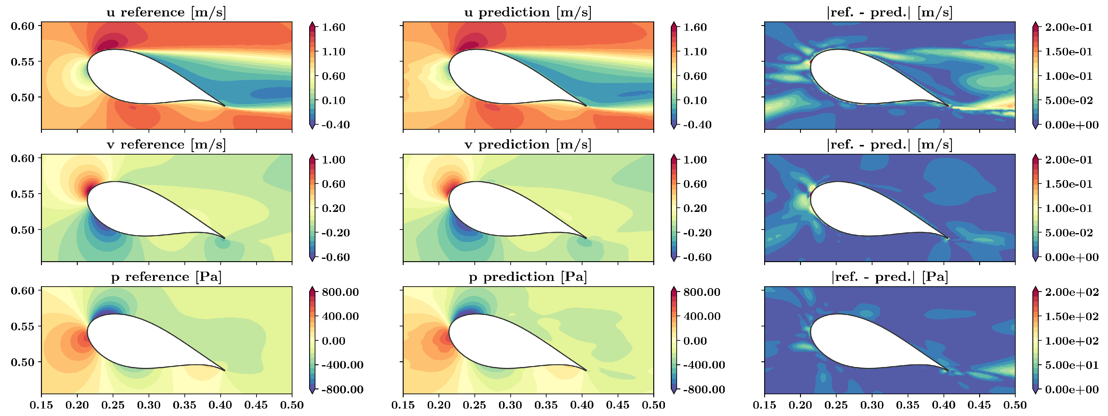
Figure 9 exhibits a comparison of the PINN predictions with the CFD results for an AoA of 12.5°. At this angle, no labeled data were provided during the training and, hence, the predictions represent an interpolation. The PINN correctly captured the low separation that was less pronounced than at an AoA of 15.0°. Furthermore, all relevant flow features were predicted. The mean deviations of the axial velocity between PINN and CFD were 3 . 7 × 10 3 m/s which represents 0.37% of the reference inlet velocity.
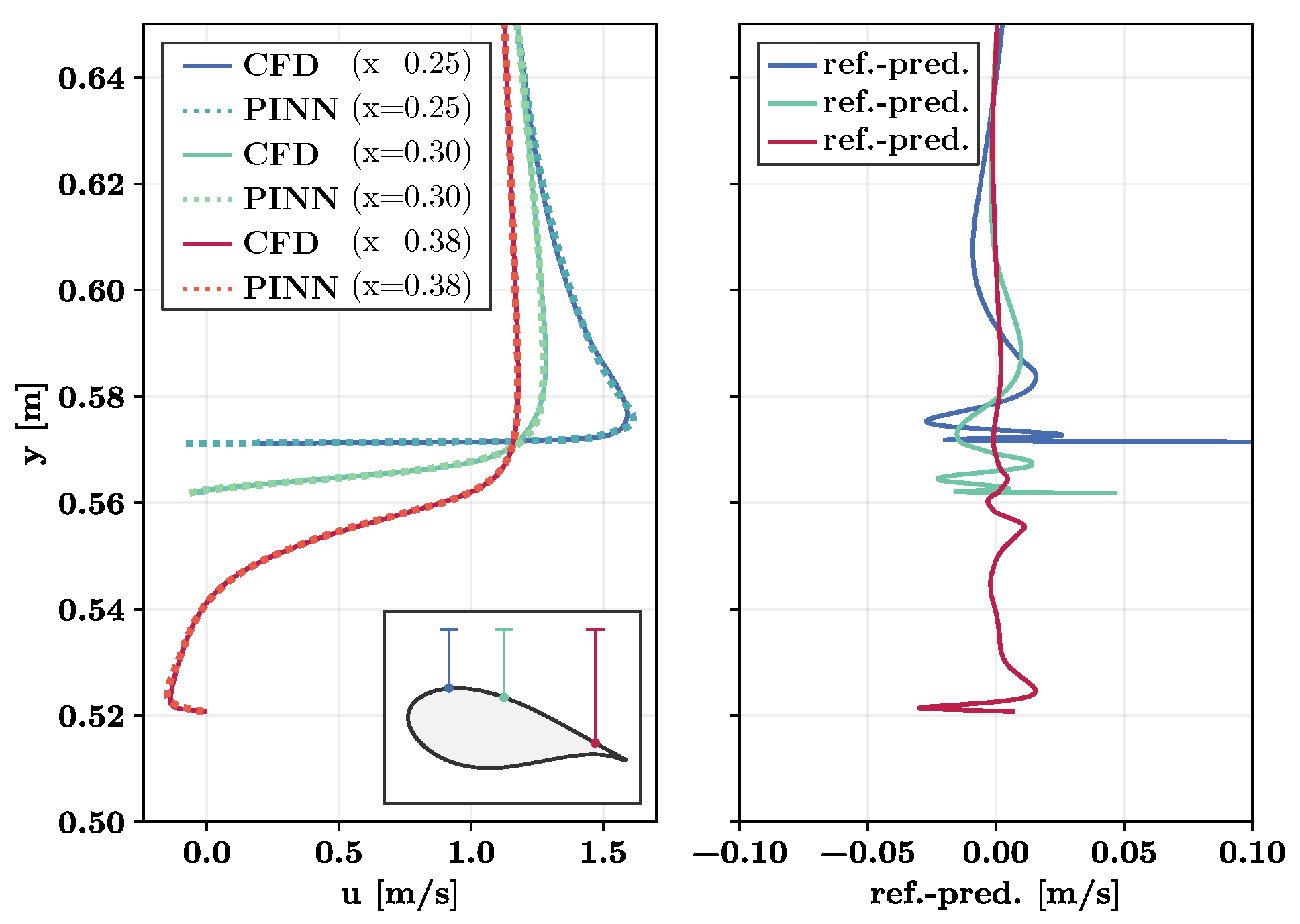
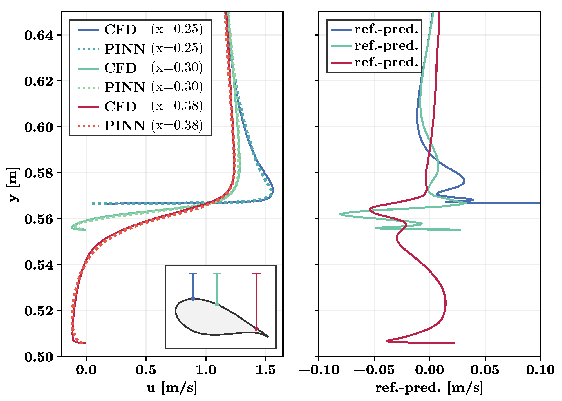
Figure 10 presents an evaluation of the prediction accuracy for several vertical lines positioned on the suction surface of the airfoil. The predicted attached and separating boundary layers were in favourable agreement with the reference data. The absolute deviation between PINN and CFD were mostly below 0.02 m/s which represents 2% of the reference inlet velocity.

5.3. Extrapolation at an AoA of 17.5°

Figure 11 compares the results at an AoA of 17.5°. This represents an extrapolation of the PINN as provision of labeled training data was restricted to lower AoA. The predictions featured the separation with the recirculating flux, the high speed regions, the stagnation regions, as well as the boundary layer. The PINN successfully predicted the progressed flow separation occurring at this AoA. The mean deviations of the axial velocity from the CFD results were 7 . 1 × 10 3 m/s which represents 0.71% of the reference inlet velocity.
Figure 12 displays a comparison of the results for several vertical lines positioned on the suction surface. As for the other AoA, the attached and separating boundary layer was captured accurately by the PINN and even the reversal of flow direction close to the surface at x = 0 . 3 m was depicted. However, the deviations from the CFD results were greater than for the interpolation at 12.5°.

5.4. Evaluation of lift and drag

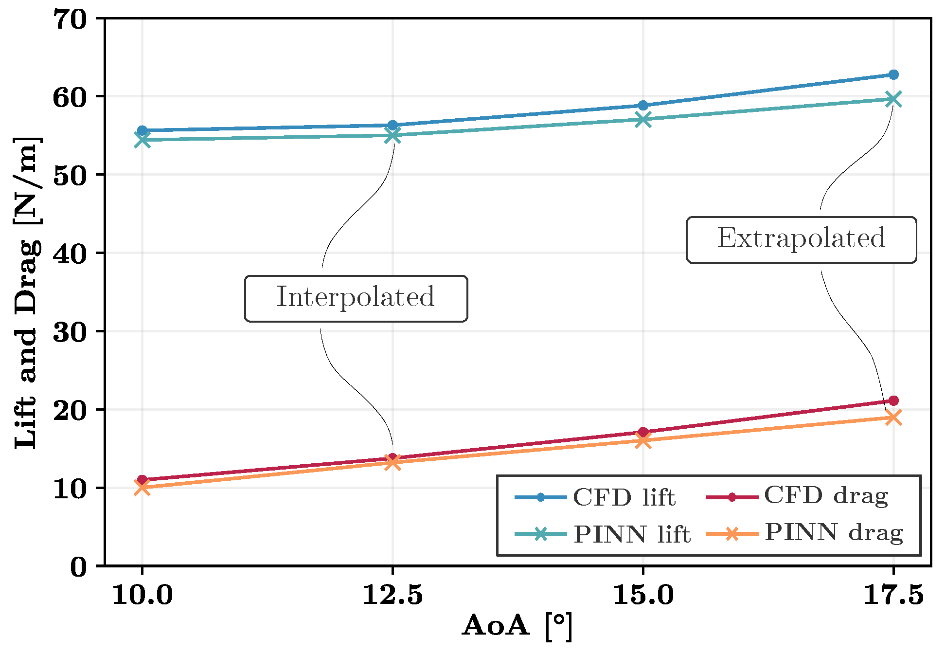
The PINN-based multidimensional surrogate method presented here can be used to obtain integral quantities for parameterized geometries, such as aerodynamic forces. Figure 13 exhibits the lift and drag results based on pressure and viscous stresses as predicted by the PINN in comparison with the CFD results. Lift L and drag D were calculated as follows:
L = C d F y p n ^ y d C + τ i j n ^ d C for i = 2
D = C d F x p n ^ x d C + τ i j n ^ d C for i = 1
where d F x and d F y are the resulting forces in x and y direction acting on the discrete surface element d C , n ^ x and n ^ y denote the x and y components of the surface normal vector n ^ of d C , and τ i j is the viscous stress tensor of an incompressible fluid:
τ i j = μ u i ¯ x j + u j ¯ x i
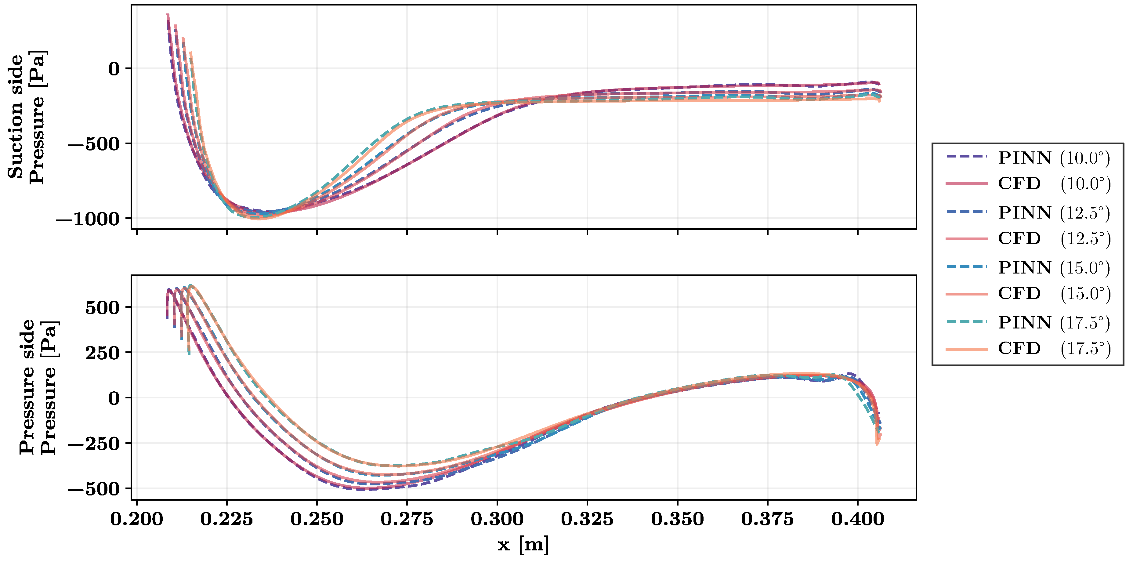
The derivations of the velocity field with respect to the coordinates were obtained using the automatic differentiation (AD) applied on the trained PINN. As seen in Figure 13, the PINN results were subject to a small bias error resulting in a slight underestimation of the lift and drag forces. Overall, the PINN predictions compared favorably with the CFD results for interpolations as well as extrapolations from the training data set. The PINN reproduced the increasing lift and drag forces as well as the decreasing lift-to-drag ratio correctly. A supplementary illustration concerning the pressure distribution on the airfoil surfaces is given in the Appendix.

5.5. Accuracy of the method

The results show that it is possible to create multidimensional surrogate models of turbulent flows with the PINN-based method proposed here. For all AoA investigated, the NN predicted the existence of the stagnation point, an attached or separated flow, boundary layers, the high-speed region on the suction surface of the airfoil, and the high- and low-pressure regions around the airfoil. Consequently, the velocity and pressure fields matched the simulated reference fields. Hence, all dominant flow phenomena could be reproduced by the neural network for variable AoA. This finding is in accordance with the results by Wandel et al. [28]. As distinguished from the approach used here, they trained a convolutional PINN that takes the vector potential as an input. This indicates that different types of PINN can be used successfully for multidimensional surrogate models.
Although the important flow phenomena could be reproduced, the predictions exhibited deviations from the reference solution. This especially accounted for high gradient regions such as the low-speed area of the stagnation point and the boundary layer on the suction side near to the leading edge. As can be seen in Figure 8 and Figure 9, the velocity field of the stagnation point was erratic and exhibited intermittent regions of high and low velocity. These results were associated with the Reynolds number and were much less pronounced at the lower Reynolds numbers investigated in our sensitivity analysis. Moreover, the boundary layer comprised only a small fraction of the training domain and, hence, was difficult to train.
The prediction accuracy varied for different AoA. For cases with available simulated labeled training data and interpolations, the solution accuracy was superior. The results showed nonetheless that accurate interpolations as well as extrapolations of the flow field are possible and even the onset and progression of flow separation could be predicted by a PINN.

5.6. Challenges and Limitations

Several publications reported excellent agreement between PINN predictions and reference solutions [11,12,19]. However, in other cases a PINN might only be capable to capture the correct solution to some extent.
One limitation is associated with the achievable errors of the prediction. The root of these errors lies in the numerical traits of the posed optimization problem characterized by parameters such as PDE, BC, activation function, network architecture, optimizer, learning rate, training points, and loss function. In case of a corresponding numerically difficult non-convex loss landscape, the optimizer might not reach the global minimum and a corresponding small optimization error. Besides, the choice of attributes such as the network architecture or the activation function corresponds with approximation and generalization errors. Jin et al. [22] investigated the effect of the training point sampling, the optimizer, and the network size on these errors for several fluid dynamic cases and obtained low errors. While there are error estimates guaranteeing the smallness of the error, this only pertains if the global minimum is found by the optimizer and if the C 1 norm of the underlying solution is small [33]. Consequently, PINN predictions have been shown to be subject to larger errors for flow fields with sharp gradients [34]. From the results of this work, this is also visible, especially for the case of the k- ω model. Here, the complexity of the nonlinear transport equations as well as the sharp gradients caused by the elevated Reynolds number of 1 × 10 5 co-occurred and no physically plausible predictions were attainable. In Section 5.8, we describe methods to potentially reduce this issue.
In this work, we used labeled simulated data for the training. In many publications, PINNs were used to predict the flow field without any labeled training data [12,14,19,22,23]. However, the Reynolds numbers of the investigated flows were below 300 and, hence, laminar. Sun et al. [19] observed that the error of the prediction of a pipe flow increased with Reynolds number. For the Reynolds number investigated in this work, especially the boundary layer and the stagnation point region were challenging to be predicted in a satisfying manner and labeled training data were necessary to obtain an acceptable error. In fact, the amount as well as the distribution of the training data were crucial factors to the success of the training. The presented example demonstrates the necessity to support the PINN with training data in small high gradient regions. This finding is supported by the results of Pioch et al. who observed that the training of a Reynolds-averaged turbulent flow field failed when no labeled training data were provided [27]. Therefore, the availability of labeled training data either from simulations or experiments is another limitation of the PINN method used here when applied to high Reynolds numbers.

5.7. Turbulence modeling

The pseudo-Reynolds turbulence modeling approach used here differs from the two-equation turbulence models typically used in CFD. For two-equation turbulence models such as the k- ϵ or the k- ω model, two transport equations need to be solved to obtain solutions for turbulent kinetic energy and dissipation rate [35]. In contrast, for the pseudo-Reynolds stress model, no equation is prescribed. Instead, the PINN is trained to predict the output in a way that the RANS equations are satisfied. This could lead to wrong predictions for velocity and pressure. Nonetheless, in the work presented here, the predicted velocity and pressure fields were in good agreement with the simulations. To some extent, this can be attributed to the employment of simulated training data with which the correct values were prescribed at several positions in the flow domain. Harmening et al. [36] also applied the pseudo-Reynolds method to a high-Reynolds flow around a square and found favorable agreements with CFD results. Furthermore, Eivazi et al. [25] applied a similar approach and reported very good agreements with simulations without using any labeled training data inside the domain.
For the training using the k- ω model, the transport equations for k and ω added to the complexity of the system of PDEs that needed to be modeled by the PINN. In fact, the k- ω model suffered from stability problems which could be attributed to Eq. (9). Bounding the predictions of k and ω stabilized the training but the results still were unfavorable, as shown in Figure 7. In a study of the flow around a backward-facing step, Pioch et al. [27] obtained favorable results using the k- ω model. However, the Reynolds number used by Pioch et al. was 5 . 1 × 10 3 while the Reynolds number of this work was 1 × 10 5 . More work needs to be done concerning two-equation models and their limitations and successful training conditions.

5.8. Potential methodological improvements

The discussed levels of accuracy as well as the limitations of the method lead to the question of possible methodological improvements. As discussed above, other types of NN might outperform the feedforward type that was used here. Many investigations used convolutional or U-Net PINNs [20,21,23,28,37]. On one side, those networks have the advantage that important features of the geometry can be identified by the autoencoder part of the NN. On the other side, convolutional neural nets process two- or three-dimensional maps as input and output and hence require significantly more weights and biases. This increases the computational costs for training. Other suitable types of NN could be a (modified) Fourier feature NN or DeepONet [24,38,39].
In this work, the boundary conditions were trained by penalizing any violation with a higher loss. Hence, the BC are not satisfied exactly after training. This can lead to small fluxes through the wall resulting in losses of mass and momentum through the wall [27]. A possible solution could be hard boundary enforcement [19]. With this approach, the exact value is enforced at the boundary using a specifically designed distance function. However, obtaining the distance function might be difficult for complex geometries [19]. Moreover, special care must be taken to prescribe only solutions that comply the law of the wall [40].
As reported by Krishnapriyan et al. [41], high parameter values in the PDE, such as large convection coefficients, might impose limitations in the learning capability of PINNs. One proposed solution could be curriculum regularization [41]. With this approach, the PINN is trained in several steps of increased numerical difficulty. Krishnapriyan et al. reported errors decreased by one to two orders of magnitude using the curriculum regularization method [41]. This method is interesting as the convection terms also dominate the PDEs for high Reynolds flows. Another promising incremental method is ensemble learning which utilizes multiple networks trained in a sequence to yield a superior outcome [42].
To increase the accuracy in small regions one could apply the residual adaptive refinement (RAR) method proposed by Lu et al. [30]. Using this method, additional training points for the PDEs are added to the training set in regions of large residuals. Wu et al. [43] investigated several sampling methods and found that residual-based adaptive distribution (RAD) and residual-based adaptive refinement with distribution (RAR-D) provided superior accuracy with fewer residual points when compared to non-adaptive distribution methods.
The labeled training points are another factor affecting the accuracy. The amount of training data positively correlated with the achieved accuracy, as shown by the sensitivity analysis of this work. The distribution of the points was a second major factor. This is visible in Figure 9 and Figure 11 which illustrate the effect of the training data positioning on the predicted stagnation point region. Note that the depicted quality of the predicted stagnation point is improvable by introducing more training points in that area. Cai et al. [44] trained a PINN to predict a shock wave problem and obtained good results using 7000 points for the PDEs, 3000 labeled training data for the density gradient and 800 labeled training data for the velocity. The procedure applied by Cai et al. gives a conception of a training point distribution that could yield an ideal highly accurate prediction of the stagnation point.
Weight factors of the composed loss terms can be set a priori, as done here, or adjusted during training. Xiang et al. [45] trained a PINN to solve the incompressible Navier Stokes equations using a self-adaptive loss function method that adjusts the losses based on a Gaussian probabilistic model. They reported an increased accuracy. A similar approach has been applied by Li et al. [46]. Wang et al. [47] proposed a method that adaptively adjusts the loss weights using the eigenvalue of the neural tangent kernel of the PINN.
Another method to increase the accuracy of the PINN in small areas could be a distributed PINN. Dwivedi et al. [48] applied a distributed PINN to predict the stationary flow in a lid-driven cavity at a low-Reynolds number. They distributed the flow domain in several cells. The flow in every cell then was predicted with separate PINN that were interconnected using interface conditions. The method has also been deployed by Shukla et al. [49].

5.9. Future work

As discussed above, the proposed PINN-based surrogate modeling approach could possibly be improved in accuracy by several methods. Future work should be put into testing and comparing the methods mentioned above, especially concerning high Reynolds numbers. For those investigations, the improvement of the prediction of important flow phenomena such as the boundary layer and the stagnation point should be focused. Furthermore, development of strategies to reduce the required amount of labeled training data are vital. Additionally, the model needs to be enhanced to three-dimensional flows.

6. Summary and conclusions

In this work, we trained a fully-connected feedforward PINN to predict the Reynolds-averaged flow field around the DU99W350 airfoil for arbitrary AoA between 10.0° and 17.5°. The PINN was trained with simulated data randomly drawn from a CFD grid for angles of attack of 10.0° and 15.0°. Additionally, satisfaction of the boundary conditions as well as the RANS equations were trained on the coordinates of a second CFD grid.
A sensitivity analysis was conducted investigating the Reynolds number, the amount and distribution of labeled training data, as well as the turbulence model. The error grew non-linearly with increasing Reynolds number and the PINN yielded accurate solutions over a range of Reynolds numbers only in case the problem was scaled varying the viscosity. It was shown that a minimum of labeled training data for supervised learning was required to obtain satisfying solutions at the Reynolds number of 1 × 10 5 . Furthermore, the sampling of training data from the coordinates of a CFD grid exhibited superior results when compared with other non-adaptive sampling strategies. The k- ω model yielded unfavorable predictions while the equation-free pseudo-Reynolds stress model agreed favorably with the reference data.
The predictions of the PINN trained for variable AoAs exhibited good agreement with the reference data for interpolations between the training data as well as extrapolations outside of the labeled training data set. The predictions exhibited excellent agreement even within the separating boundary layer on the suction surface of the airfoil. However, the results also revealed challenges in predicting high gradient regions accurately. This was evident for the stagnation point at the leading edge of the airfoil.
The results of this work demonstrate the capability of feedforward PINNs to predict the Reynolds-averaged flow field around variable geometries at high Reynolds numbers.

Author Contributions

Jan Hauke Harmening: Conceptualization; Investigation; Methodology; Software; Project administration; Writing – original draft; Writing – review and editing. Fabian Pioch: Conceptualization; Investigation; Methodology; Software; Project administration; Visualization; Writing – review and editing. Lennart Fuhrig: Investigation; Software; Writing – review and editing. Franz-Josef Peitzmann: Resources; Supervision; Writing – review and editing. Dieter Schramm: Supervision; Writing – review and editing. Ould el Moctar: Supervision; Writing – review and editing.

Data Availability Statement

The data that support the findings of this study are available from the corresponding authors upon reasonable request.

Conflicts of Interest

The authors have no conflicts to disclose.

Appendix A. Supplementary illustrations

Figure A1 shows the losses for PDEs, BCs, and data during the training of the multidimensional model. Figure A2 exhibits the coordinates for the training of PDEs and BCs for an AoA of 15.0°. Figure A3 illustrates the different training point positioning strategies applied in the sensitivity analysis. Figure A4 shows the pressure distribution for CFD and PINN on the airfoil surface, divided into pressure and suction side for all AoA.
Figure A1. Loss during training for the final model and the iteration with the lowest global NMSE.
Preprints 72180 g0a1
Figure A2. Illustration of the training point coordinates for the training of the PDEs at an AoA of 15.0°.
Preprints 72180 g0a2
Figure A3. Exemplary illustration of the randomly drawn training point coordinates of the labeled data at an AoA of 15.0°. Left: points randomly drawn from a uniform grid; middle: points uniformly placed along several vertical and horizontal lines; right: points randomly drawn from the coordinates of a CFD grid.
Preprints 72180 g0a3
Figure A4. Pressure distribution on the airfoil surfaces for several AoA.
Preprints 72180 g0a4

References

  1. M. Fernández-Delgado, M. S. Sirsat, E. Cernadas, S. Alawadi, S. Barro, and M. Febrero-Bande. An extensive experimental survey of regression methods. Neural networks : The official journal of the International Neural Network Society, 111:11–34, 2019. [CrossRef]
  2. A. Pinkus. Approximation theory of the mlp model in neural networks. Acta Numerica, 8:143–195, 1999. [CrossRef]
  3. A. C. Comrie. Comparing neural networks and regression models for ozone forecasting. Journal of the Air & Waste Management Association, 47(6):653–663, 1997. [CrossRef]
  4. G. Heuvelmans, B. Muys, and J. Feyen. Regionalisation of the parameters of a hydrological model: Comparison of linear regression models with artificial neural nets. Journal of Hydrology, 319(1-4):245–265, 2006. [CrossRef]
  5. Y. Kim and H. Oh. Comparison between multiple regression analysis, polynomial regression analysis, and an artificial neural network for tensile strength prediction of bfrp and gfrp. Materials (Basel, Switzerland), 14(17), 2021. [CrossRef]
  6. A. Shrestha and A. Mahmood. Review of deep learning algorithms and architectures. IEEE Access, 7:53040–53065, 2019. [CrossRef]
  7. N. Thuerey, K. Weißenow, L. Prantl, and X. Hu. Deep learning methods for reynolds-averaged navier–stokes simulations of airfoil flows. AIAA Journal, 58(1):25–36, 2020. [CrossRef]
  8. I. E. Lagaris, A. Likas, and D. I. Fotiadis. Artificial neural networks for solving ordinary and partial differential equations. IEEE transactions on neural networks, 9(5):987–1000, 1998. [CrossRef]
  9. M. Raissi, P. Perdikaris, and G. E. Karniadakis. Physics informed deep learning (part i): Data-driven solutions of nonlinear partial differential equations, 2017. [CrossRef]
  10. M. Raissi, P. Perdikaris, and G. E. Karniadakis. Physics informed deep learning (part ii): Data-driven discovery of nonlinear partial differential equations, 2017. [CrossRef]
  11. M. Raissi, P. Perdikaris, and G. E. Karniadakis. Physics-informed neural networks: A deep learning framework for solving forward and inverse problems involving nonlinear partial differential equations. Journal of Computational Physics, 378:686–707, 2019. [CrossRef]
  12. M. Raissi, A. Yazdani, and G. E. Karniadakis. Hidden fluid mechanics: Learning velocity and pressure fields from flow visualizations. Science (New York, N.Y.), 367(6481):1026–1030, 2020. [CrossRef]
  13. V. Sekar, Q. Jiang, C. Shu, and B. C. Khoo. Accurate near wall steady flow field prediction using physics informed neural network (pinn), 2022. [CrossRef]
  14. R. Laubscher and P. Rousseau. Application of a mixed variable physics-informed neural network to solve the incompressible steady-state and transient mass, momentum, and energy conservation equations for flow over in-line heated tubes. Applied Soft Computing, 114:108050, 2022. [CrossRef]
  15. Q. Zhu, Z. Liu, and J. Yan. Machine learning for metal additive manufacturing: Predicting temperature and melt pool fluid dynamics using physics-informed neural networks. Computational Mechanics, 67(2):619–635, 2021. [CrossRef]
  16. H. Ouyang, Z. Zhu, K. Chen, B. Tian, B. Huang, and J. Hao. Reconstruction of hydrofoil cavitation flow based on the chain-style physics-informed neural network. Engineering Applications of Artificial Intelligence, 119:105724, 2023. [CrossRef]
  17. S. Wang, X. Yu, and P. Perdikaris. When and why pinns fail to train: A neural tangent kernel perspective. Journal of Computational Physics, 449:110768, 2022. [CrossRef]
  18. S. Xu, Z. Sun, R. Huang, D. Guo, G. Yang, and S. Ju. A practical approach to flow field reconstruction with sparse or incomplete data through physics informed neural network. Acta Mechanica Sinica, 39(3), 2023. [CrossRef]
  19. L. Sun, H. Gao, S. Pan, and J.-X. Wang. Surrogate modeling for fluid flows based on physics-constrained deep learning without simulation data. Computer Methods in Applied Mechanics and Engineering, 361:112732, 2020. [CrossRef]
  20. R. Wang, K. Kashinath, M. Mustafa, A. Albert, and R. Yu. Towards physics-informed deep learning for turbulent flow prediction. In R. Gupta, Y. Liu, M. Shah, S. Rajan, J. Tang, and B. A. Prakash, editors, Proceedings of the 26th ACM SIGKDD International Conference on Knowledge Discovery & Data Mining, pages 1457–1466, New York, NY, USA, 08232020. ACM.
  21. Y. Zhu, N. Zabaras, P.-S. Koutsourelakis, and P. Perdikaris. Physics-constrained deep learning for high-dimensional surrogate modeling and uncertainty quantification without labeled data. Journal of Computational Physics, 394(1):56–81, 2019. [CrossRef]
  22. X. Jin, S. Cai, H. Li, and G. E. Karniadakis. Nsfnets (navier-stokes flow nets): Physics-informed neural networks for the incompressible navier-stokes equations. Journal of Computational Physics, 426:109951, 2021. [CrossRef]
  23. H. Ma, Y. Zhang, N. Thuerey, X. Hu, and O. J. Haidn. Physics-driven learning of the steady navier-stokes equations using deep convolutional neural networks, 2021. [CrossRef]
  24. O. Hennigh, S. Narasimhan, M. A. Nabian, A. Subramaniam, K. Tangsali, Z. Fang, M. Rietmann, W. Byeon, and S. Choudhry. Nvidia simnet™: An ai-accelerated multi-physics simulation framework. In M. Paszynski, D. Kranzlmüller, V. V. Krzhizhanovskaya, J. J. Dongarra, and P. M. Sloot, editors, Computational Science – ICCS 2021, volume 12746 of Lecture Notes in Computer Science, pages 447–461. Springer International Publishing, Cham, 2021.
  25. H. Eivazi, M. Tahani, P. Schlatter, and R. Vinuesa. Physics-informed neural networks for solving reynolds-averaged navier–stokes equations. Physics of Fluids, 34(7):075117, 2022. [CrossRef]
  26. H. Xu, W. Zhang, and Y. Wang. Explore missing flow dynamics by physics-informed deep learning: The parameterized governing systems. Physics of Fluids, 33(9):095116, 2021. [CrossRef]
  27. F. Pioch, J. H. Harmening, A. M. Müller, F.-J. Peitzmann, D. Schramm, and O. el Moctar. Turbulence modeling for physics-informed neural networks: Comparison of different rans models for the backward-facing step flow. Fluids, 8(2):43, 2023. [CrossRef]
  28. N. Wandel, M. Weinmann, and R. Klein. Teaching the incompressible navier-stokes equations to fast neural surrogate models in 3d. Physics of Fluids, 33(4):047117, 2021. [CrossRef]
  29. C. J. Arthurs and A. P. King. Active training of physics-informed neural networks to aggregate and interpolate parametric solutions to the navier-stokes equations. Journal of Computational Physics, 438:None, 2021. [CrossRef]
  30. L. Lu, X. Meng, Z. Mao, and G. E. Karniadakis. Deepxde: A deep learning library for solving differential equations. SIAM Review, 63(1):208–228, 2021. [CrossRef]
  31. D. C. Wilcox. Reassessment of the scale-determining equation for advanced turbulence models. AIAA Journal, 26(11):1299–1310, 1988. [CrossRef]
  32. J. Jonkman, S. Butterfield, W. Musial, and G. Scott. Definition of a 5-mw reference wind turbine for offshore system development, 2009. [CrossRef]
  33. T. De Ryck, A. D. Jagtap, and S. Mishra. Error estimates for physics-informed neural networks approximating the Navier–Stokes equations. IMA Journal of Numerical Analysis, 2023.
  34. S. Mishra and R. Molinaro. Estimates on the generalization error of physics-informed neural networks for approximating a class of inverse problems for pdes. IMA Journal of Numerical Analysis, 42(2):981–1022, 2022. [CrossRef]
  35. D. C. Wilcox. Formulation of the k-w turbulence model revisited. AIAA Journal, 46(11):2823–2838, 2008. [CrossRef]
  36. J. H. Harmening, F. Pioch, and D. Schramm. Physics informed neural networks as multidimensional surrogate models of cfd simulations. In Machine Learning und Artificial Intelligence in Strömungsmechanik und Strukturanalyse, Wiesbaden, Germany, 16.–17. may, pages 71–80. NAFEMS, may 2022.
  37. Y. Kim, Y. Choi, D. Widemann, and T. Zohdi. A fast and accurate physics-informed neural network reduced order model with shallow masked autoencoder. Journal of Computational Physics, 451:110841, 2022. [CrossRef]
  38. L. Lu, P. Jin, G. Pang, Z. Zhang, and G. E. Karniadakis. Learning nonlinear operators via deeponet based on the universal approximation theorem of operators. Nature Machine Intelligence, 3(3):218–229, 2021. [CrossRef]
  39. S. Wang, H. Wang, and P. Perdikaris. On the eigenvector bias of fourier feature networks: From regression to solving multi-scale pdes with physics-informed neural networks. Computer Methods in Applied Mechanics and Engineering, 384:113938, 2021. [CrossRef]
  40. D. Spalding et al. A single formula for the law of the wall. Journal of Applied Mechanics, 28(3):455–458, 1961.
  41. A. Krishnapriyan, A. Gholami, S. Zhe, R. Kirby, and M. W. Mahoney. Characterizing possible failure modes in physics-informed neural networks. In M. Ranzato, A. Beygelzimer, Y. Dauphin, P.S. Liang, and J. Wortman Vaughan, editors, Advances in Neural Information Processing Systems, volume 34, pages 26548–26560. Curran Associates, Inc, 2021.
  42. Z. Fang, S. Wang, and P. Perdikaris. Ensemble learning for physics informed neural networks: A gradient boosting approach, 2023. [CrossRef]
  43. C. Wu, M. Zhu, Q. Tan, Y. Kartha, and L. Lu. A comprehensive study of non-adaptive and residual-based adaptive sampling for physics-informed neural networks, 2022. [CrossRef]
  44. S. Cai, Z. Mao, Z. Wang, M. Yin, and G. E. Karniadakis. Physics-informed neural networks (pinns) for fluid mechanics: A review. Acta Mechanica Sinica, 37(12):1727–1738, 2021. [CrossRef]
  45. Z. Xiang, W. Peng, X. Zheng, X. Zhao, and W. Yao. Self-adaptive loss balanced physics-informed neural networks for the incompressible navier-stokes equations, 2021. [CrossRef]
  46. S. Li and X. Feng. Dynamic weight strategy of physics-informed neural networks for the 2d navier-stokes equations. Entropy (Basel, Switzerland), 24(9), 2022. [CrossRef]
  47. H. Wang, Y. Liu, and S. Wang. Dense velocity reconstruction from particle image velocimetry/particle tracking velocimetry using a physics-informed neural network. Physics of Fluids, 34(1):017116, 2022. [CrossRef]
  48. V. Dwivedi, N. Parashar, and B. Srinivasan. Distributed physics informed neural network for data-efficient solution to partial differential equations, 2019. [CrossRef]
  49. K. Shukla, A. D. Jagtap, and G. E. Karniadakis. Parallel physics-informed neural networks via domain decomposition. Journal of Computational Physics, 447:110683, 2021. [CrossRef]
Figure 1. Features of the simulated reference flow field around the DU99W350 airfoil. 1: Stagnation point; 2: high velocity region on the suction surface; 3: boundary layer on the airfoil surface; 4: separated shear layer; 5: wake and recirculative vortices; 6: constant free flow; 7: high velocity region on the pressure surface.
Preprints 72180 g001
Figure 2. Architecture of the deployed neural network.
Preprints 72180 g002
Figure 3. Illustration of the multidimensional hypercube training domain and the corresponding boundary conditions and training data.
Preprints 72180 g003
Figure 4. Results of the sensitivity analysis concerning the training accuracy for different Reynolds numbers. The relative deviations are presented on a logarithmic scale.
Preprints 72180 g004
Figure 5. Results of the sensitivity analysis concerning the amount of labeled training data.
Preprints 72180 g005
Figure 6. Results of the sensitivity analysis concerning the distribution method of labeled training data.
Preprints 72180 g006
Figure 7. Results of the sensitivity analysis concerning different turbulence models. The absolute deviations are presented on a logarithmic scale.
Preprints 72180 g007
Figure 8. Results and absolute error of the axial velocity around the DU99W350 airfoil at an angle of attack of 15.0° using a PINN in comparison with the reference data. Note that for this angle of attack, reference data were provided for the training of the PINN.
Preprints 72180 g008
Figure 9. Results and absolute error of velocity and pressure around the DU99W350 airfoil at an angle of attack of 12.5° using a PINN in comparison with the reference data. Note that for this angle of attack, no reference data were provided for the training of the PINN.
Preprints 72180 g009
Figure 10. Results and residual of the axial velocity on the suction surface of the DU99W350 airfoil at an angle of attack of 12.5° using a PINN in comparison with the reference data. Left: axial velocity; right: residual between PINN and CFD results. Note that for this angle of attack, no reference data were provided for the training of the PINN.
Preprints 72180 g010
Figure 11. Results and absolute error of velocity and pressure around the DU99W350 airfoil at an angle of attack of 17.5° using a PINN in comparison with the reference data. Note that for this angle of attack, no reference data were provided for the training of the PINN.
Preprints 72180 g011
Figure 12. Results and residual of the axial velocity on the suction surface of the DU99W350 airfoil at an angle of attack of 17.5° using a PINN in comparison with the reference data. Left: axial velocity; right: residual between PINN and CFD results. Note that for this angle of attack, no reference data were provided for the training of the PINN.
Preprints 72180 g012
Figure 13. Lift and drag results for the DU99W350 airfoil as predicted by the PINN in comparison with the CFD results.
Preprints 72180 g013
Table 1. PINN training parameters.
Parameter Value/setting
Architecture five hidden layer
with 128 neurons each
Optimizer Adam, L-BFGS-B
Epochs 30,000 (Adam)
Learning rate 10 3 (10,000 epochs)
and 10 4 (20,000 epochs)
activation function tanh
Number training points n b + n d 3200
Number training points n d 800 at 10.0° and 15.0° each
Number training points n e 6277
Loss terms weighting factors λ b = 1 , λ d = 100 , λ e = 1
Disclaimer/Publisher’s Note: The statements, opinions and data contained in all publications are solely those of the individual author(s) and contributor(s) and not of MDPI and/or the editor(s). MDPI and/or the editor(s) disclaim responsibility for any injury to people or property resulting from any ideas, methods, instructions or products referred to in the content.
Copyright: This open access article is published under a Creative Commons CC BY 4.0 license, which permit the free download, distribution, and reuse, provided that the author and preprint are cited in any reuse.
Prerpints.org logo

Preprints.org is a free preprint server supported by MDPI in Basel, Switzerland.

Subscribe

© 2024 MDPI (Basel, Switzerland) unless otherwise stated