
You are currently viewing a beta version of our website. If you spot anything unusual, kindly let us know.
Preprint
Article
Improved Curve–Flattening for Flexible Space Robotics
Altmetrics
Downloads
225
Views
138
Comments
0


This version is not peer-reviewed
Intelligent Systems and Robotics
Abstract
Compared with the traditional robots on earth, space robotics present additional difficulties including complicated, multi–body dynamics (including anti–resonances absent with earthly robotic systems), space environmental forces and torques, communication delays, and high expense. Pointing accuracy requirements necessitate control algorithms that can accommodate flexible, multi–body dynamics particularly. The high cost of placing systems in space drives necessarily lightweight systems lacking structural stiffness. Natural frequencies of space robot vibration are often so low, the act of implementing control torques causes structural resonance. Seeking improved performance, this manuscript introduces and compares a dozen options, revealing seventy–percent reduction in tracking error may be achieved with only ten percent increase in control effort. Prequel work recommended tracking sinusoidal shaped trajectories while structurally filtering the first mode’s resonance and anti–resonance. The future research recommended in that prequel is manifest in this present work which recommends a simpler system of lower order, eliminating the notch compensation of the first resonance while no longer compensating the first anti–resonance.
Keywords:
Subject: Engineering - Aerospace Engineering
1. Introduction
Contemporary engineers in NASA’s Marshall Space Flight Center [6] proclaim devotion to reduce the cost of space exploration from ten thousand dollars per pound (to orbit) to tens of dollars per pound in forty years. In addition to cost, technical performance is a common area of concern for all systems’ development. Technical performance of highly flexible space robotics is complicated by an inability to avoid structural resonances simply by increasing structural stiffness (making the robot heavier and thereby more costly).
1.1. Review of the literature
Driven by the high cost of spaceflight, space robots seek to simultaneously maintain low mass and volume, and also increase fuel efficiency, [6] addressed in this work by monitoring control usage as a figure of merit [7]. The flexible spacecraft simulator laboratory (in Figure 1b) is a prototype to simulate space robotic manipulation to provide future possibilities. Several mathematical approaches are manifest in the literature for modeling traditional robotics. [8] Expressed in Euclidean space [9], every particle can be modeled based on internal and external constraints. Chasle’s theorem [10] combines Newton’s second law [11] and Euler’s equation [12], motion states of space robots can be defined in six degrees of freedom [13].
A modern method for space robotics is displayed in Figure 2, containing the control system designing by using the mathematical model and techniques such as feedback control [14] and feedforward control sometimes necessitating system identification [15]. The approach generally involves creating a model of the robot and its environment, and then designing a control system that uses sensors to measure the robot’s state and actuator command to control its movements.
Designing the feedback control involves designing the close–loop system to adjust the robot’s behavior according to Peter Ian Corke [16]. Classical control techniques such as PID control [17] are commonly used in robot control, which are well–established and have been used on a wide variety of systems for decades. Such a system can adjust the output of a system in response to changes in the inputs or setpoints, while maintaining stability and minimizing oscillations in the movement trajectory. A commonly used modern method seeking to minimize a performance measure is the linear quadratic regulator. Reference [18] elaborates the LQR (linear quadratic regulator) helps to design the control of linear time–invariant systems for tasks such as trajectory tracking, stabilization, and manipulation.
Beside the feedback control, there is also feedforward control existing. In the journal [19], the authors briefly explained the basic idea of such control. The feedforward control would be more useful in the situations where the robot’s movements are predictable, so it can also be called the open–loop control. Figure 2 illustrates such instantiations, where the subfigures display SIMULINK® simulations of those instantiations.
Potentially, there are also plenty of method to modeling and control the robot in the future. People are still doing the deeper investigation on that. One example is the artificial intelligence (AI). There is one journal states [20] that in medicine field, more people are willing to do more research to apply AI on the surgery robot. By utilizing machine learning algorithms, robots can be trained to learn different environment and tasks. Another example is the Internet of Things (IoT), which enables the physical devices to interconnect with software to exchange data. For now, there’re some improvement and achievement on the robot arm [21], which can remotely control and monitor the robot anywhere.
The goal of presenting the framework of the robotics control modeling method is to inspire and stimulate latter scientists and engineers to concentrate more on the field of space robotics. Developing the service robots on orbit to do the inspection and replenishment is urgent and necessary, which is a gigantic milestone in the process of space exploration by human.
1.2. State of the art benchmarks
Pre–existing commercial electronics (sensors and controllers) accompany the purchase of commercial surgical robotic systems, and retroactive improvement of such electronics can prove difficult in reaction to newly developed methods. Improvements of the commercially purchased systems must have improvements somehow “imposed”. Recent research [22] proposes imposing performance improvements upon pre–existing, common systems by establishing a comparative benchmark for comparing eight alternatives. One contemporary update (velocity control) of a classical feedback control was used as a comparative benchmark for a modern approach derived using terminal transversality of the endpoint Lagrangian, adjoint equations, and Hamiltonian minimization, together often referred to as systems theory of Soviet mathematician Lev Pontryagin.
Accessibility of robots is proposed to be improved by mimicking the surface characteristics of geckos [23] by the design of various synthetic adhesives: thermoplastic, dry fibrillary, electrostatic. A narrative review of spinal surgical robots using both traditional and modern robotics to aid skill acquisition was described in [24], emphasizing the range of training platforms’ measures of proficiency available to ensure confident preparation.
Ankle syndesmosis reduction forces were quantified in [25] to improve accuracy of image–guided robotic assistant design requirements, where six manipulation techniques were compared with respect to a cadaveric ankle’s directions of reduction. Hands-free speech–based communication with surgical robotics assistants was elaborated in reference [26] which proposed a description format of robot skill to facilitate voice control programming applications.
Robotic orthopedic surgery is largely focused on high volume arthroplasty procedures, while relatively less attention is paid to ankle and foot surgery robots. The study in [27] presented artificial intelligence with deep learning modeling enhancements for preclinical and translational robotic utilization for foot and ankle surgery. Open surgery palpitation assessment directly (tactilely) is impeded during robot-assisted, minimally invasive surgery. Analyzing extractable surgical instrument information (e.g., structural vibrations) during indirect palpitation, classifiers supported by k–nearest neighbors and vector machine provided 96.00% and 99.67% information respectfully. [28] “Palpation is an intuitive examination procedure in which the kinesthetic and tactile sensations of the physician are used”. [29]
Such structural vibrations are key to the research presented in this manuscript.
Reference [30] illustrate effectiveness of soft–robotic two-network pneumatic grippers, where independent work can lead to effective grasping. A larger output force (compared to single pneumatic networks) was achieved while simultaneously retaining desired bending deformation abilities. Another illustration is offered in [31], where experimental validation illustrates less than 8% deviations in agreement with the calculated bending angle.
Active control modeling is used to address tracking error induced in pneumatic artificial muscles by hysteretic nonlinearities. Active modeling control is offered in reference [32] as a method of compensation. The hysteresis is described by a reference model with induced errors, while modeling errors and system states are estimated by an unscented Kalman filter. Experiments valided some ability to ameliorate transient overshoot and settling.
Such overshoot and settling are key to the research presented in this manuscript.
A review of electrical soft actuators that proves to be quite focused in offered by reference [33] for response, controllability, softness, and compactness asserted a lack of soft robotics electromagnetic motor equivalent, despite such being accepted and a well-known single actuator for applications over a broad range.
According to reference [34] introducing soft parts into otherwise rigid robots can overcome limitations of rigid structures, taking advantage of complex controls of relatively low force exertion, especially applicable to space industry applications necessitating novel (ultra) lightweight, low-volume, systems that is deployable upon purchase. The investigation studied hybrid manipulators with rigid joints and flexible links where the flexible, inflatable behavior was treated as a pseudo–rigid body.
Such rigid structure and flexible links are key to the research in this manuscript.
In reference [35], a hierarchical–controlled exoskeletal systems are controlled with series elastic actuators with force feedback of motor current from encoders on motor and joints using a networking approach merging low and high-level controller updates and synchronization. Control of robotic arms using reference paths is proposed in [36] using two degrees of autonomy utilizing electromyography and force sensor feedback, where the main limitations were limited range of motion and cost. Flexibility of bendable devices was highlighted in [37] for transsphenoidal pituitary surgery to avoid organ damage proposing an automatic segmentation, U–Net–based algorithm for both internal carotid arteries and optical nerves using both angiography images and patient computed tomography for training.
Providing a stable surgical view, adjustable stiffness, flexible endoscopes can repel from the surrounding tissues and organs different external loads, deemed necessary in minimally invasive surgery according to [38]. Pneumatic soft actuators have an antagonistic mechanism are proposed to adjust actuator stiffness. Adjustable stiffness can manipulate vibrational frequencies and shapes of fixed–mass robotic arms.
Such stiffness of flexible robotics links are key to the research in this manuscript.
A system is proposed in [39] for using both computer vision and machine learning for tactile detection on a forearm’s sleeve on a large scale with a cylindrical design, whose dimensions are akin human biceps or forearms. An artificial neural network with supervised learning achieved accuracy higher than 80%. Such performance is accepted as a contemporary benchmark.
A single–incision, robotic laparoscopic surgical system is proposed in [40], which consists of an external driving device and an inner laparoscopic robot. The control of robot position and orientation are provided outside the abdominal wall by a magnetic field generated by the driving device. The electromagnetism model and the mechanical model were used to design and build a prototype laparoscopic robot system. Translational, rotational, and deflection motion were demonstrated experimentally, but the accuracy was verified only in open loop.
Muli-agent structural flexibility is often represented in modal analysis, where the difficulties achieving optimal control include complex interaction among agents. A learning mechanics and an action value function is proposed in reference [41] obtaining the optimal agent decisions maximizing a posteriori based on the hidden Markov random field model using the optimal equivalent action of the neighborhood of a multi–agent system. The property of convergence is claimed to be able to approach the value of global Nash equilibrium, while experimental results merely show that the method can reduce the complexity of the agents’ interaction description, while the performance can be improved. Seeking mathematically minimum control effort, so–called whiplash compensation was recently proposed [42] whose provenance lies in optimization using Pontryagin’s treatment of Hamiltonian systems [43].
An adaptive iterative learning control (AILC) law based on Hamilton’s principle was proposed for two–link rigid–flexible coupled manipulators with time–varying disturbances and input constraints in [44]. Simulations were given that merely proved convergence of the control objectives under the adaptive iterative learning control law. An adaptive robust attitude tracking control scheme is proposed in [45] for near space vehicles expressed as a stochastic nonlinear system. A multi–dimensional Taylor polynomial network is utilized to handle the system uncertainties, and the nonlinear disturbance observer is designed to estimate the external disturbances, while the mere closed–loop system stability in the sense of probability was analyzed based on stochastic Lyapunov stability theory, while numerical simulations were offered to demonstrate the feasibility of the proposed tracking control scheme.
Reference [46] is the key prequel to the research presented in this manuscript. Infrastructure monitoring, inspection, repair, and replacement in space using very light weight flexible space robots are proposed to address a key challenge of the presence of flexible resonant modes at frequencies so low as to reside inside typical feedback controller bandwidths. Such conditions imply the very action of sending control signals to the ultra–light weight robotics will cause structural resonance. Like the earlier cited references, commanded trajectories are a key part of the analysis presented, and over ninety percent performance improvement in trajectory tracking errors is validated for single–sinusoidal trajectory shaping with a corollary benefit of preparing future research into applying deterministic artificial intelligence [47] whose current instantiation relies on single–sinusoidal, autonomous trajectory generation. While noteworthy improvements in tracking errors were achieved, the curve–flattening methods emphasized stability, while the results presented here mimic reference [46], but re–attempt the approach emphasizing tracking errors, embodying overshoot and settling.
1.3. Novelties presented
- The best tracking (mean) error performance (best efficacy against overshoot and settling) is achieved using full modal compensation of the first three flexible modes plus a bandpass filter of the fourth flexible mode’s anti–resonance.
- The best tracking error deviation was achieved with merely compensation of the rigid body mode plus bandpass filtering of the first flexible mode’s anti–resonance.
- The lowest control cost was achieved by the same method listed in item #2: merely compensation of the rigid body mode plus bandpass filtering of the first flexible mode’s resonance.
1.4. Highlighting controversial and diverging hypotheses
The key prequel research [46] recommended rigid–body compensation plus full compensation of only the first flexible mode (based upon resultant system order with sinusoidal–shaped trajectories), the experimental results presented in this manuscript indicate superior tracking error performance (without addressing commanded trajectories) may be achieved with a simpler system of lower order, eliminating the notch compensation of the first resonance.
2. Materials and Methods
In this section, it contains all the equations that use to get the calculation results, including both rigid and flexible body, and the control system with parameters. By following the subsections in order, the modeling results can be gathered step by step, which is shown in the Section 3.
2.1. Rigid Body Dynamics
Rigid body is the starting point to consider for space robotics modeling by using the Newton’s second law of motion [11] to get the 6 DOF [12]. The following part in this subsection introduces some basic modeling information as well as the relationship between Hamiltonian and Newton’s law.
Equation (1) represents the basic Newton’s law of motion that provide the relationships between force, mass, and acceleration. And Equation (2) shows the relationship between torque and angular acceleration. Both are describing the non–rotating situations. Equation (3) and (4) are expressed in rotational conditions and describe the replenishment and assembly manipulation for the space robot working on orbit. Based on Equation (1) to (4), it can be combined to get 6 degrees of freedom.

Table 1.
Table of proximal variables and nomenclature 1.
| Variable / acronym |
Definition | Variable / acronym |
Definition |
|---|---|---|---|
| F | Vector sum of external forces | Vector sum of external torque | |
| J |
Moments of inertia Velocity relative to reference frame |
|
Position relative to the reference frame Angular velocity |
1 Such tables are offered throughout the manuscript to aid readability.
Figure 3.
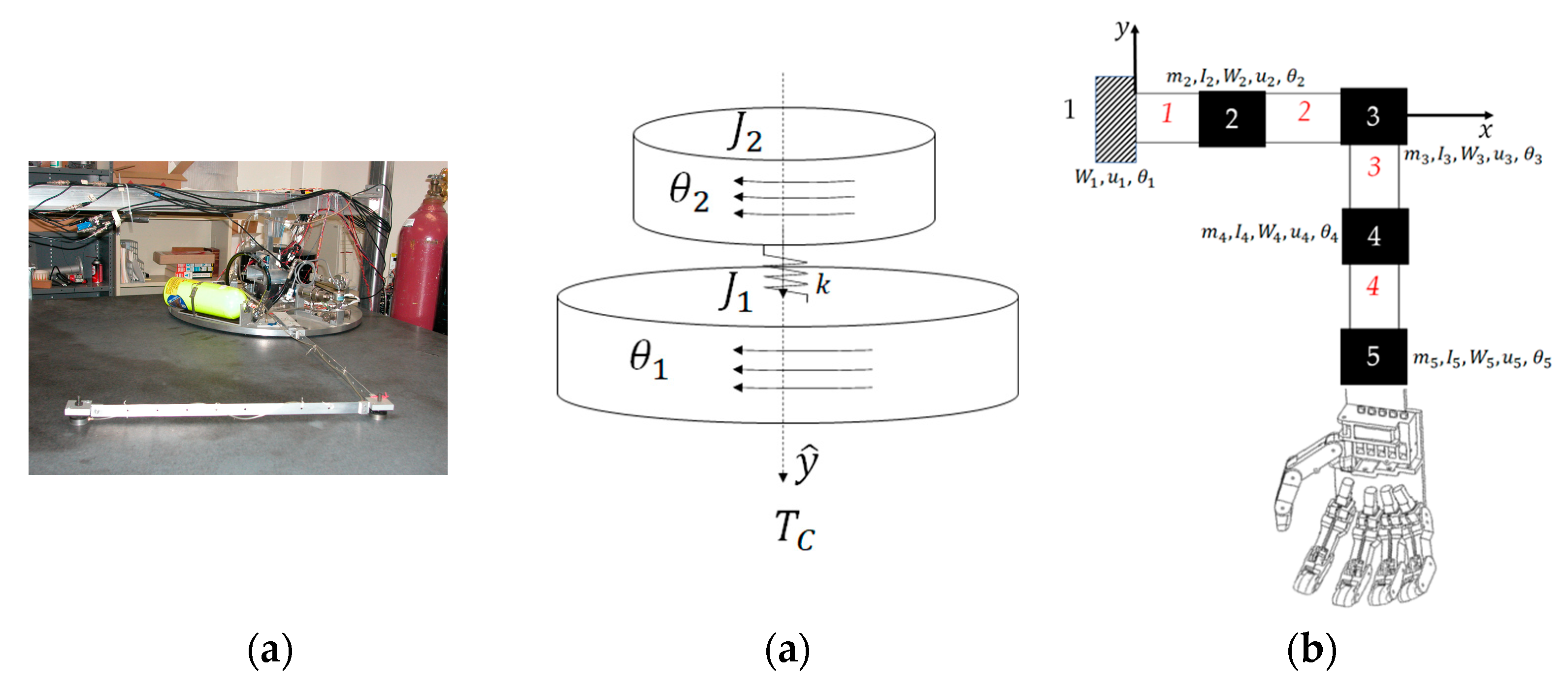
(a) U.S. Naval Postgraduate School simulate a very lightweight, low–stiffness, free–floating robot on a planar air–bearing table in autonomous robotic laboratory. [3] U.S. Department of Defense photographs and imagery, unless otherwise noted, are in the public domain [4]. Images courtesy U.S. Department of Defense [5]; (b) modeling and analysis of the flexible robot depicted in (a) discretized into four nodes depicted in (c) of the mass moment of inertias through appended to the rigid body depicted in (b) as , where in (b) represents the sum of constituent inertias at nodes 2–5 in (c).
Figure 3.
(a) U.S. Naval Postgraduate School simulate a very lightweight, low–stiffness, free–floating robot on a planar air–bearing table in autonomous robotic laboratory. [3] U.S. Department of Defense photographs and imagery, unless otherwise noted, are in the public domain [4]. Images courtesy U.S. Department of Defense [5]; (b) modeling and analysis of the flexible robot depicted in (a) discretized into four nodes depicted in (c) of the mass moment of inertias through appended to the rigid body depicted in (b) as , where in (b) represents the sum of constituent inertias at nodes 2–5 in (c).
Equation (5) states the expression for the Lagrange method, where the potential energy is related to the height displacement and kinetic energy is related to the motion velocity. The left side of the Equation (6) is the representation for the Hamiltonian and the first term of the right side is Lagrangian. By doing the differentiation and minimization, it can produce the Euler–Lagrange equation shown in Equation (7). With certain steps of algebraic arrangement, Equation (7) can be modified to Newton’s Law shown in Equation (8).
Table 2.
Table of proximal variables and nomenclature 1.
| Variable/acronym | Definition | Variable/acronym | Definition |
|---|---|---|---|
| Hamiltonian | Lagrangian |
1 Such tables are offered throughout the manuscript to aid readability.
2.2. Flexible Body Dynamics
Every flexible body can be modeled as a certain number of nodes. The rotational and translational equation for rigid body explained in Section 2.1.1 can be applied to each node classified. The number of the equations generated equals to the number of the nodes. Therefore, in Section 2.2, it introduces the how the flexible body modeled based on the equations used in rigid body.
When modeling the Flexible body dynamics, the equation of motion can be produced by Euler–Lagrange’s method. It combined with the Kinetic Energy and Potential Energy together to apply the most situations. The expression for the Kinetic energy is shown in the Equation (9) where is the particle velocity on rigid body, is the particle velocity on flexible body, and is the reaction wheel particle velocity.
2.3. Modal System Identification
This section introduces the how the nodal degrees of freedom can be set up. It states the equation modification to get the torque relationship, which can be applied to the control topology calculation shown in Figure 4.
When modeling the Flexible robot, every node in the system should follow Newton’s second law of motion to get equation with the damping in accordance with equation (10).
where the [M] is the global mass matrix, [C] is the global stiffness matrix, and [F] is the force matrix.
Here, when considering the nodal degrees of freedom, it should be constrained to be zero for both the flexible and rigid bodies. In such situation, only the corner node for the flexible body is considered, so the degrees of freedom for the horizontal and vertical direction are replaced by the angular rotation. Thus, the Newton’s second law can be modified as the combination of rotational form and the rigid–elastic coupling method as shown in the Equation (11), where is the sum of the disturbance torques.
After rearranging the modified equation, the angular acceleration of the system rotation angle can be represented as the Equation (12) states.
Table 3.
Table of proximal variables and nomenclature 1.
| Variable/ acronym |
Definition | Variable/ acronym |
Definition |
|---|---|---|---|
| Mass matrix | Stiffness matrix | ||
| Acceleration in generalized displacement coordinates | Principal moment of inertia with respect to z-axis | ||
| Force vector | Coupling term for rigid-elastic |
1 Such tables are offered throughout the manuscript to aid readability.
2.4. Classical Second–Order Structural Filtering
In this section, it uses an example equation to introduce a PID type of control system with the Laplace transformation. In Figure 4, the SIMULINK model used to get the result is presented with the filter function provided. The commonly used controller in feedback control is the PID control, which uses proportional, integral, and Derivative components to make up the control algorithm. Equation (13) states the close–loop equation example for the proportional and velocity components controller. By doing the Laplace transformation, Equation (12) can be converted into Equation (14). It can not only guide on the performance specification, e.g., stability, overshoot, settling time, etc., but also help to get the structural filtering to adapt the compensation with the natural frequency of the system.
Equation (15) provides the transfer function for the structural filters used to augment the system compensation. It defines the frequencies and the damping ratio for the zeros and poles. According to the equation, the steady–state gain, maximum gain, and the phase can be measured numerically. Based on the parameters: ,and , the point that occur maximum lead and lag can also be found.
Table 4.
Table of proximal variables and nomenclature 1.
| Variable/acronym | Definition | Variable/acronym | Definition |
|---|---|---|---|
| Active damping | Active stiffness | ||
| Feedforward | |||
1 Such tables are offered throughout the manuscript to aid readability.
2.5. Simulation Parameters
The simulation (depicted in Figure 4) and the Appendix are created by MATLAB/SIMULINK with version r2022b. The results are shown in the Section 3.
Figure 4.
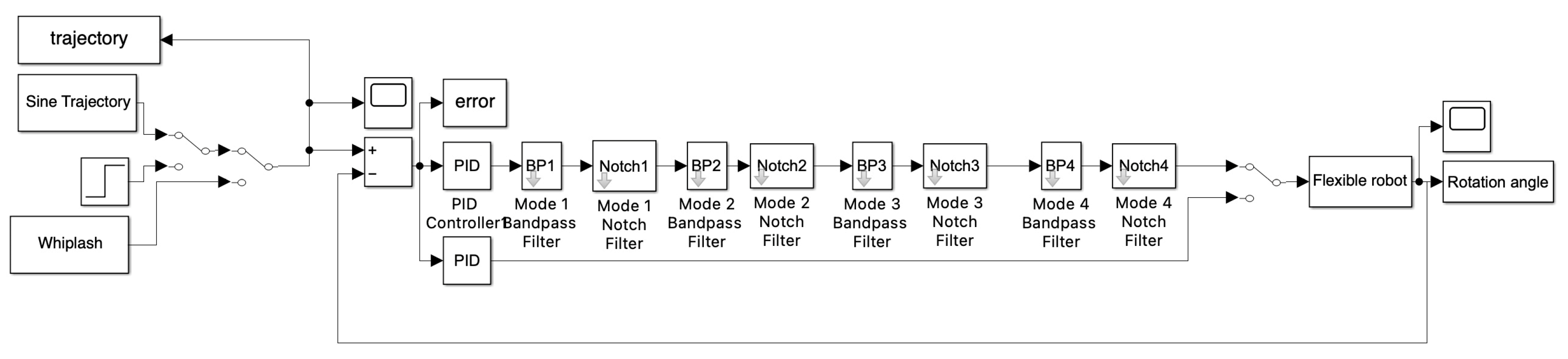
Control topology used in this article with proportional, integral, and derivative control combined with the second–order structural filter, which are bandpass (BP) and notch. It is designed by using the Equation (14) with the parameters of the filter.
Figure 4.
Control topology used in this article with proportional, integral, and derivative control combined with the second–order structural filter, which are bandpass (BP) and notch. It is designed by using the Equation (14) with the parameters of the filter.
3. Results
In this section, the simulation result and the numerical result will be provided. It simulates the performance with two types of the structural filter added by using the Equation (15) provided in Section 2. This article will concentrate on three sets of data, which are cost, tracking error, and tracking error deviation.
3.1. Simulation results with structural filters (bandpass & notch) for the first flexible mode.
The system is augmented with structural filters, so the frequencies and the damping ratio is modified by the filters to reach the goal of “flatten the curve” in the frequency response plot. In this case, three types of system are compared. First, only a bandpass filter is added to the system for the first anti–resonant spike. Second, only a notch filter is added to the system for the first resonant spike. Last, both the bandpass and the notch filter are added together to the system. Figure 5 shows the graphical result for these three systems and the numerical result is listed in Table 5. The graphical line for the first and the last system are almost overlap.
3.2. Simulation results with structural filter (bandpass & notch) for the first four flexible modes.
The goal for this case is to compare the influence for the cost and the error as adding the mode. Figure 6 represents the graphic result for the first four flexible modes separately to reach the goal of “flatten the curve”. Table 6 shows the numerical result. As shown in the graph, the last four situations are overlapped.
3.3. Simulation with Structural Filter (Bandpass and Notch) for the First Three Flexible Modes and First Four Bandpass.
Due to the better performance when adding bandpass only in mode 1, in this case, it compares the performance when adding the full modes and an extra bandpass filter. The graphic result for the four system is shown in the Figure 7 and the numerical results are shown in the Table 7. It clearly states in the graph that the lines for the last three systems are overlapped.
4. Discussion
Besides the comparison about the stability and the trajectory–tracking performance to “flatten the curve”, the cost and the tracking error are two essential factors to be considered with. In this section, all the results are gathered and formed a table to compare the percentage change by comparing with the most “basic” system, PID only. For the cost, the lower, the better performance, but for the tracking error, the lower, the better performance.
As shown in the Table 8, the highlighted number are the best performed value compared vertically. Even though the last system has the lowest tracking error, the cost is almost the highest. However, if only compensate with bandpass 1, the cost only increases 10% and the tracking error can decrease 71.28%. Therefore, the system with only first bandpass perform the best.
| Recommendation: Use the bandpass filter at the first anti-resonance in first flexible mode with step input to compensate the flexible space robots. |
Recommended future research
Based on the result data calculated, the most effective way of controlling is PID with one bandpass. To further determine the effectiveness of the result got here, it would be useful to implement the same controller onto the other type of the robots to see if it is still effective on the different platforms.
The research effort described in this manuscript enables future research into applying deterministic artificial intelligence [47] whose current instantiation relies on single–sinusoidal, autonomous trajectory generation, but to-date has not been implemented on highly flexible space robotics, where self-awareness statements may now be formulated using the results in this manuscript, while optimal learning [48] might prove efficacy towards variable system mass during grasping and grappling and also time-varying learning of robot resonance and anti-resonant frequencies.
References
- Nile, R.; First Humanoid Robot In Space Receives NASA Government Invention of the Year. 17 June 2015. Available online: https://www.nasa.gov/mission_pages/station/research/news/invention_of_the_year (accessed on 17 February 2023).
- NASA. NASA Image Use Policy. 2022. Available online: https://gpm.nasa.gov/image-use-policy (accessed on 14 April 2023).
- Naval Postgraduate School, Flexible Spacecraft Simulator Laboratory. Available online: https://nps.edu/web/srdc/laboratories (accessed on 12 April 2023).
- Use of Department of Defense Imagery. Available online: https://www.defense.gov/Help-Center/Article/Article/2762906/use-of-department-of-defense-imagery/#:~:text=Department%20of%20Defense%20photographs%20and,use%2C%20subject%20to%20specific%20guidelines (accessed on 14 April 2023).
- Defense Imagery Management Operations Center. Public Use Notice of Limitations. Available online: https://www.dimoc.mil/resources/limitations/ (accessed on 14 April 2023).
- Marshall Spaceflight Center, Advanced Space Transportation Program: Paving the Highway to Space. Available online: https://www.nasa.gov/centers/marshall/news/background/facts/astp.html (accessed on 15 January 2022).
- Curiosity Bot, Advantages and disadvantages of using Robots instead of Astronauts. Available online: https://mycuriositybot.wordpress.com/2019/02/18/advantages–and–disadvantages–of–using–robots–instead–of–astronauts/ (accessed on 18 February 2019).
- Armanini, C.; Boyer, F.; Mathew, A.T.; Duriez, C.; Renda, F. Soft Robots Modeling: A Structured Overview. IEEE Trans. Robot. 2023, 39, 1728–1748. [Google Scholar] [CrossRef]
- Encyclopaedia Britannica, Britannica, Euclidean Space. Available online: https://www.britannica.com/science/Euclidean–space (accessed on 10 October 2022).
- Sands, T. Comparison and Interpretation Methods for Predictive Control of Mechanics. Algorithms 2019, 12, 232. [Google Scholar] [CrossRef]
- Newton, I. Principia, Jussu Societatis Regiæ ac Typis Joseph Streater; Cambridge University Library: London, UK, 1687. [Google Scholar]
- Mazalov, V.; Parilina, E. The Euler-Equation Approach in Average-Oriented Opinion Dynamics. Mathematics 2020, 8, 355. [Google Scholar] [CrossRef]
- A.C.M. Operations, What–Are–the–6–Degrees–of–Freedom, Industrial Inspection & Analysis (IIA). Available online: https://industrial–ia.com/what–are–the–6–degrees–of–freedom–6dof–explained/ (accessed on 21 March 2023).
- Doyle, J.; Francis, A.; Tannenbaum, A. Feedback Control Theory; Dover: Mineola, NY, USA, 2009. [Google Scholar]
- Johansson, R.; Robertsson, A.; Nilsson, K.; Verhaegen, M. State-space system identification of robot manipulator dynamics. Mechatronics 2000, 10, 403–418. [Google Scholar] [CrossRef]
- Corke, P, “High–performance visual closed–loop robot control,” thesis.
- Li, Y.; Ang, K.H.; Chong, G. PID control system analysis and design. IEEE Control. Syst. 2006, 26, 32–41. [Google Scholar] [CrossRef]
- Bemporad, A.; Morari, M.; Dua, V.; Pistikopoulos, E. The explicit linear quadratic regulator for constrained systems. Automatica 2002, 38, 3–20. [Google Scholar] [CrossRef]
- Tao, K; Kosut, R; Aral, G, “Learning feedforward control,” Proceedings of 1994 American Control Conference –ACC ’94.
- Chang, T.C.; Seufert, C.; Eminaga, O.; Shkolyar, E.; Hu, J.C.; Liao, J.C. Current Trends in Artificial Intelligence Application for Endourology and Robotic Surgery. Urol. Clin. North Am. 2020, 48, 151–160. [Google Scholar] [CrossRef]
- Fu, S; Bhavsar, P, “Robotic Arm Control based on internet of things,” 2019 IEEE Long Island Systems, Applications and Technology Conference (LISAT), 2019.
- Sands, T. Inducing Performance of Commercial Surgical Robots in Space. Sensors 2023, 23, 1510. [Google Scholar] [CrossRef]
- Sikdar, S.; Rahman, M.H.; Siddaiah, A.; Menezes, P.L. Gecko–Inspired Adhesive Mechanisms and Adhesives for Robots—A Review. Robotics 2022, 11, 143. [Google Scholar] [CrossRef]
- McDonnell, J.M.; Ahern, D.P.; Doinn, T.; Gibbons, D.; Rodrigues, K.N.; Birch, N.; Butler, J.S. Surgeon proficiency in robot-assisted spine surgery. Bone Jt. J. 2020, 102-B, 568–572. [Google Scholar] [CrossRef]
- Gebremeskel, M.; Shafiq, B.; Uneri, A.; Sheth, N.; Simmerer, C.; Zbijewski, W.; Siewerdsen, J.H.; Cleary, K.; Li, G. Quantification of manipulation forces needed for robot-assisted reduction of the ankle syndesmosis: an initial cadaveric study. Int. J. Comput. Assist. Radiol. Surg. 2022, 17, 2263–2267. [Google Scholar] [CrossRef] [PubMed]
- Rogowski, A. Scenario–Based Programming of Voice–Controlled Medical Robotic Systems. Sensors 2022, 22, 9520. [Google Scholar] [CrossRef] [PubMed]
- Stauffer, T.P.; Kim, B.I.; Grant, C.; Adams, S.B.; Anastasio, A.T. Robotic Technology in Foot and Ankle Surgery: A Comprehensive Review. Sensors 2023, 23, 686. [Google Scholar] [CrossRef] [PubMed]
- Sühn, T.; Esmaeili, N.; Mattepu, S.Y.; Spiller, M.; Boese, A.; Urrutia, R.; Poblete, V.; Hansen, C.; Lohmann, C.H.; Illanes, A.; Friebe, M. Vibro–Acoustic Sensing of Instrument Interactions as a Potential Source of Texture–Related Information in Robotic Palpation. Sensors 2023, 23, 3141. [Google Scholar] [CrossRef]
- Ahn, B.; Kim, Y.; Oh, C.K.; Kim, J. Robotic palpation and mechanical property characterization for abnormal tissue localization. Med Biol. Eng. Comput. 2012, 50, 961–971. [Google Scholar] [CrossRef]
- Zhang, H.; Liu, W.; Yu, M.; Hou, Y. Design, Fabrication, and Performance Test of a New Type of Soft–Robotic Gripper for Grasping. Sensors 2022, 22, 5221. [Google Scholar] [CrossRef]
- Yu, M.; Liu, W.; Zhao, J.; Hou, Y.; Hong, X.; Zhang, H. Modeling and Analysis of a Composite Structure–Based Soft Pneumatic Actuators for Soft–Robotic Gripper. Sensors 2022, 22, 4851. [Google Scholar] [CrossRef]
- Qin, Y.; Zhang, H.; Wang, X.; Han, J. Active Model–Based Hysteresis Compensation and Tracking Control of Pneumatic Artificial Muscle. Sensors 2022, 22, 364. [Google Scholar] [CrossRef]
- Ma, Z.; Sameoto, D. A Review of Electrically Driven Soft Actuators for Soft Robotics. Micromachines 2022, 13, 1881. [Google Scholar] [CrossRef]
- Palmieri, P.; Melchiorre, M.; Mauro, S. Design of a Lightweight and Deployable Soft Robotic Arm. Robotics 2022, 11, 88. [Google Scholar] [CrossRef]
- Herron, C.W.; Fuge, Z.J.; Kogelis, M.; Tremaroli, N.J.; Kalita, B.; Leonessa, A. Design and Validation of a Low–Level Controller for Hierarchically Controlled Exoskeletons. Sensors 2023, 23, 1014. [Google Scholar] [CrossRef] [PubMed]
- Chellal, A.A.; Lima, J.; Gonçalves, J.; Fernandes, F.P.; Pacheco, F.; Monteiro, F.; Brito, T.; Soares, S. Robot–Assisted Rehabilitation Architecture Supported by a Distributed Data Acquisition System. Sensors 2022, 22, 9532. [Google Scholar] [CrossRef] [PubMed]
- Song, H. –S.; Yoon, H.–S.; Lee, S.; Hong, C.–K.; Yi, B.–J. Surgical Navigation System for Transsphenoidal Pituitary Surgery Applying U–Net–Based Automatic Segmentation and Bendable Devices. Appl. Sci. 2019, 9, 5540. [Google Scholar] [CrossRef]
- Lu, Y.; Zhou, Z.; Kokubu, S.; Qin, R.; Tortós Vinocour, P.E.; Yu, W. Neural Network–Based Active Load–Sensing Scheme and Stiffness Adjustment for Pneumatic Soft Actuators for Minimally Invasive Surgery Support. Sensors 2023, 23, 833. [Google Scholar] [CrossRef] [PubMed]
- Cunha, F.; Ribeiro, T.; Lopes, G.; Ribeiro, A.F. Large–Scale Tactile Detection System Based on Supervised Learning for Service Robots Human Interaction. Sensors 2023, 23, 825. [Google Scholar] [CrossRef] [PubMed]
- Wei, H.; Li, K.; Xu, D.; Tan, W. Design of a Laparoscopic Robot System Based on Spherical Magnetic Field. Appl. Sci. 2019, 9, 2070. [Google Scholar] [CrossRef]
- Wang, H.; Yang, Y.; Lin, Z.; Wang, T. Multi–Agent Reinforcement Learning with Optimal Equivalent Action of Neighborhood. Actuators 2022, 11, 99. [Google Scholar] [CrossRef]
- Sands, T. Optimization Provenance of Whiplash Compensation for Flexible Space Robotics. Aerospace 2019, 6, 93. [Google Scholar] [CrossRef]
- Sands, T. Virtual Sensoring of Motion Using Pontryagin’s Treatment of Hamiltonian Systems. Sensors 2021, 21, 4603. [Google Scholar] [CrossRef]
- Zhang, J.; Dai, X.; Huang, Q.; Wu, Q. AILC for Rigid–Flexible Coupled Manipulator System in Three–Dimensional Space with Time–Varying Disturbances and Input Constraints. Actuators 2022, 11, 268. [Google Scholar] [CrossRef]
- Yan, X.; Shao, G.; Yang, Q.; Yu, L.; Yao, Y.; Tu, S. Adaptive Robust Tracking Control for Near Space Vehicles with Multi–Source Disturbances and Input–Output Constraints. Actuators 2022, 11, 273. [Google Scholar] [CrossRef]
- Sands, T. Flattening the Curve of Flexible Space Robotics. Appl. Sci. 2022, 12, 2992. [Google Scholar] [CrossRef]
- Huang, B.; Sands, T. Novel Learning for Control of Nonlinear Spacecraft Dynamics. J. AppliedMath 2023, 1. [Google Scholar] [CrossRef]
- Smeresky, B.; Rizzo, A.; Sands, T. Optimal Learning and Self-Awareness Versus PDI. Algorithms 2020, 13, 23. [Google Scholar] [CrossRef]
Figure 1.
(a) Space robots with cylindrical center rigid bodies and highly flexible appendages. (a) NASA’s first humanoid space robot, image credit NASA [1], Image usage is consistent with NASA policy, “NASA content (images, videos, audio, etc.) are generally not copyrighted and may be used for educational or informational purposes without needing explicit permissions.” [2]. (b) U.S. Naval Postgraduate School simulate a very lightweight, low–stiffness, free–floating robot on a planar air–bearing table in autonomous robotic laboratory. [3] U.S. Department of Defense photographs and imagery, unless otherwise noted, are in the public domain [4]. Images courtesy U.S. Department of Defense [5].
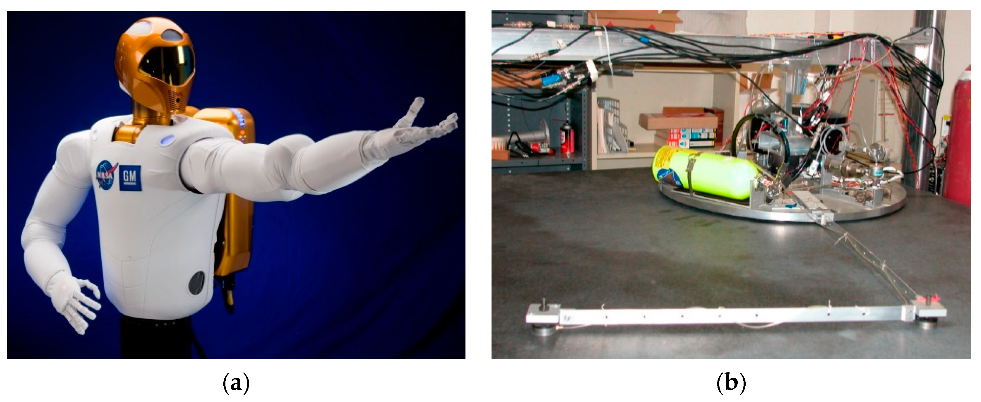
Figure 2.
(a) Space robot control topology, (b) topology of flexible space robot subsystem in (a).
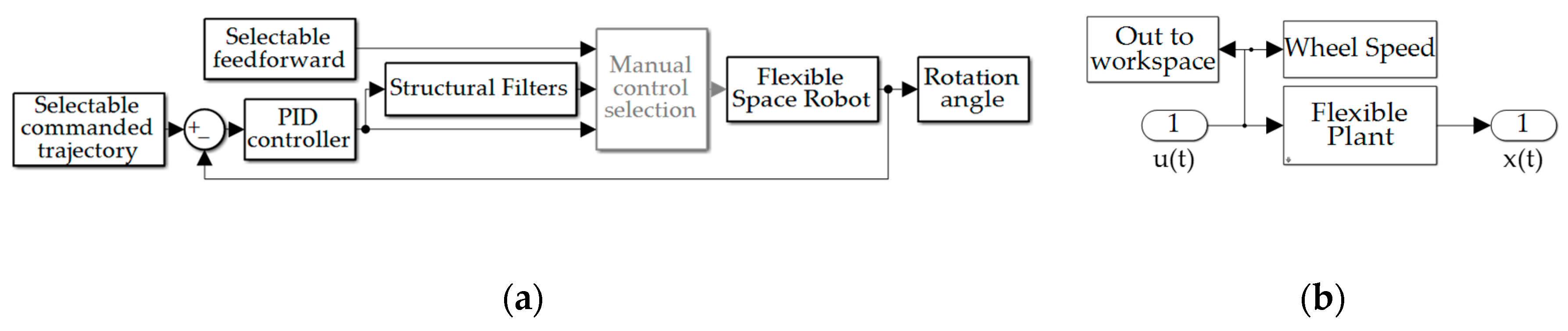
Figure 5.
Three computer simulation of control of rigid body; the compensated with Bandpass only, compensated with notch only, and the compensated with both the bandpass and notch. (a) Cost performance (b) Tracking error performance. PID + bandpass (dotted black line); PID + notch (dotted red line); PID + bandpass + notch (solid blue line).
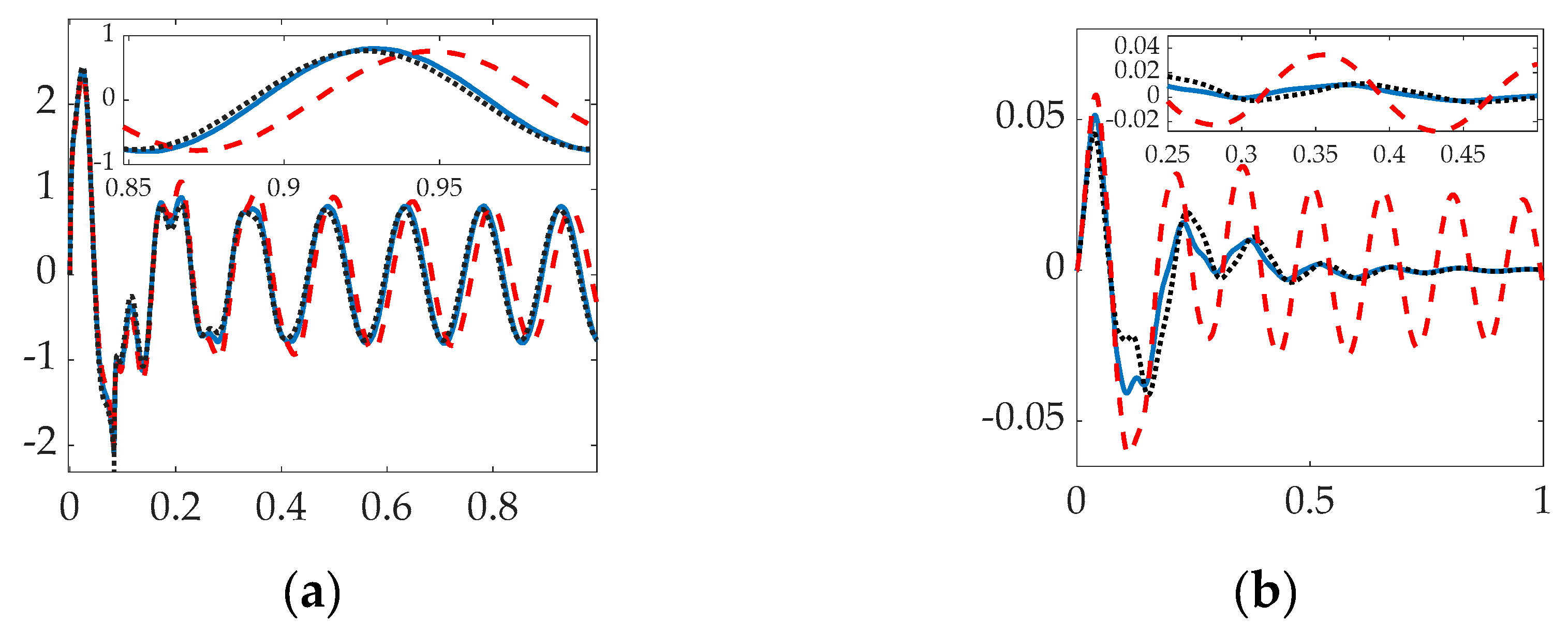
Figure 6.
Five computer simulation of control of the rigid body; compensated with first mode (Bandpass and Notch), compensated with first two modes, compensated with first three modes, and compensated with first four modes. (a) Cost performance (b) Tracking error performance. PID controlled (solid blue line); PID + mode 1 (thick dashed orange line); PID + mode 1–2 (dotted black line); PID + mode 1–3 (thick dashed green line); PID + mode 1–4 (solid red line).
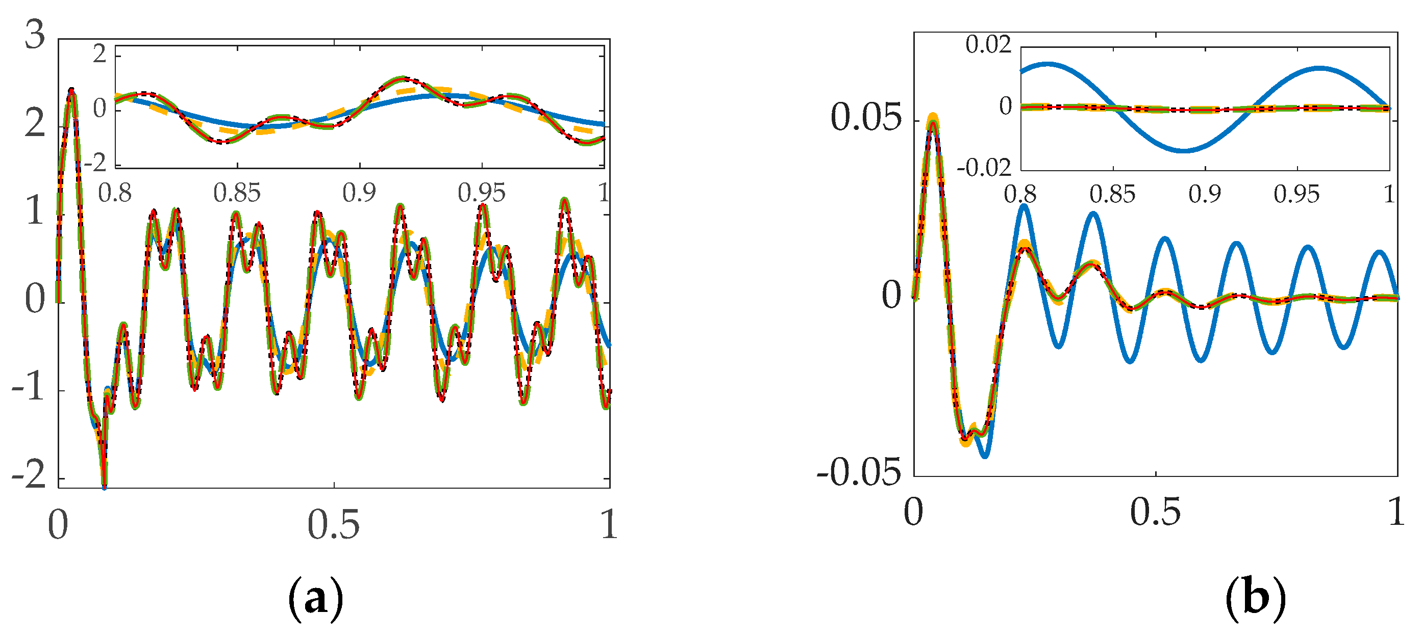
Figure 7.
Four computer simulation of control of the rigid body; the compensated with first Bandpass only, compensated with first mode and second bandpass only, compensated with first two modes and third bandpass only, and compensated with first three modes and fourth bandpass only (a) Cost performance (b) Tracking error performance. PID + bandpass 1 (solid red line); PID + mode 1 + bandpass 2 (thick solid blue line); PID + mode 1–2 + bandpass 3 (dashed black line); PID + mode 1–3 + bandpass 4 (dashed green line).
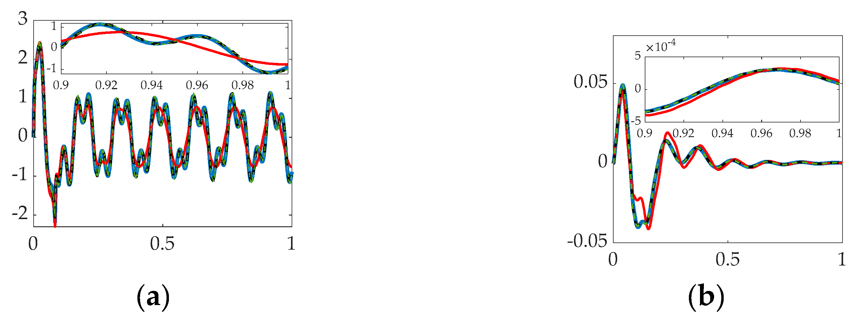
Table 5.
Rigid body & first flexible mode compensation.
| System | Cost | Tracking error mean |
Tracking Error deviation |
|---|---|---|---|
| PID + Bandpass | 8.06 | 0.00014406 | 0.014064 |
| PID + Notch PID + Bandpass + Notch |
8.9353 8.4414 |
0.000714 0.00019857 |
0.025414 0.015501 |
Table 6.
Rigid body & first four flexible mode compensation.
| System | Cost | Tracking error mean |
Tracking Error deviation |
|---|---|---|---|
| PID controlled | 7.3167 | 0.00050164 | 0.018844 |
| PID + Mode 1 PID + Mode 1–2 PID + Mode 1–3 PID +Mode 1–4 |
8.4414 9.9155 9.906 9.9054 |
0.00019857 0.00020995 –0.00026647 –0.00031746 |
0.015501 0.015452 0.014086 0.014496 |
Table 7.
Compensation of rigid body plus first three flexible modes and first four bandpass.
| System | Cost | Tracking error mean |
Tracking Error deviation |
|---|---|---|---|
| PID + bandpass 1 | 8.06 | 0.00014406 | 0014064 |
| PID + Mode 1 + bandpass 2 PID + Mode 1–2 + bandpass 3 PID + Mode 1–3 + bandpass 4 |
9.7423 9.8582 9.8914 |
0.00019832 0.00017655 0.000013948 |
0.015269 0.01524 0.01414 |
Table 8.
Percentage increased comparison based on the PID only system. Minus sign means the value is smaller than the PID only, and vice versa.
Table 8.
Percentage increased comparison based on the PID only system. Minus sign means the value is smaller than the PID only, and vice versa.
| System | Cost | Tracking Error | Tracking Error deviation |
|---|---|---|---|
| PID only PID + bandpass1 PID + notch1 PID + Mode 1 PID + Mode 1–2 PID + Mode 1–3 PID +Mode 1–4 |
– 10.16% 22.12% 15.37% 35.52% 35.38% 35.38% |
– –71.28% 42.33% –60.42% –58.15% –46.88% –36.72% |
– –23.22% 37.01% –15.60% –15.86% –23.11% –20.93% |
| PID + Mode 1 + bandpass 2 PID + Mode 1–2 + bandpass 3 PID + Mode 1–3 + bandpass 4 |
33.15% 34.74% 35.18% |
–60.47% –64.81% –97.22% |
–16.83% –16.98% –22.82% |
Disclaimer/Publisher’s Note: The statements, opinions and data contained in all publications are solely those of the individual author(s) and contributor(s) and not of MDPI and/or the editor(s). MDPI and/or the editor(s) disclaim responsibility for any injury to people or property resulting from any ideas, methods, instructions or products referred to in the content. |
© 2023 by the authors. Licensee MDPI, Basel, Switzerland. This article is an open access article distributed under the terms and conditions of the Creative Commons Attribution (CC BY) license (http://creativecommons.org/licenses/by/4.0/).
Copyright: This open access article is published under a Creative Commons CC BY 4.0 license, which permit the free download, distribution, and reuse, provided that the author and preprint are cited in any reuse.
Submitted:
29 April 2023
Posted:
30 April 2023
You are already at the latest version
Alerts
This version is not peer-reviewed
Intelligent Systems and Robotics
Submitted:
29 April 2023
Posted:
30 April 2023
You are already at the latest version
Alerts
Abstract
Compared with the traditional robots on earth, space robotics present additional difficulties including complicated, multi–body dynamics (including anti–resonances absent with earthly robotic systems), space environmental forces and torques, communication delays, and high expense. Pointing accuracy requirements necessitate control algorithms that can accommodate flexible, multi–body dynamics particularly. The high cost of placing systems in space drives necessarily lightweight systems lacking structural stiffness. Natural frequencies of space robot vibration are often so low, the act of implementing control torques causes structural resonance. Seeking improved performance, this manuscript introduces and compares a dozen options, revealing seventy–percent reduction in tracking error may be achieved with only ten percent increase in control effort. Prequel work recommended tracking sinusoidal shaped trajectories while structurally filtering the first mode’s resonance and anti–resonance. The future research recommended in that prequel is manifest in this present work which recommends a simpler system of lower order, eliminating the notch compensation of the first resonance while no longer compensating the first anti–resonance.
Keywords:
Subject: Engineering - Aerospace Engineering
1. Introduction
Contemporary engineers in NASA’s Marshall Space Flight Center [6] proclaim devotion to reduce the cost of space exploration from ten thousand dollars per pound (to orbit) to tens of dollars per pound in forty years. In addition to cost, technical performance is a common area of concern for all systems’ development. Technical performance of highly flexible space robotics is complicated by an inability to avoid structural resonances simply by increasing structural stiffness (making the robot heavier and thereby more costly).
1.1. Review of the literature
Driven by the high cost of spaceflight, space robots seek to simultaneously maintain low mass and volume, and also increase fuel efficiency, [6] addressed in this work by monitoring control usage as a figure of merit [7]. The flexible spacecraft simulator laboratory (in Figure 1b) is a prototype to simulate space robotic manipulation to provide future possibilities. Several mathematical approaches are manifest in the literature for modeling traditional robotics. [8] Expressed in Euclidean space [9], every particle can be modeled based on internal and external constraints. Chasle’s theorem [10] combines Newton’s second law [11] and Euler’s equation [12], motion states of space robots can be defined in six degrees of freedom [13].
A modern method for space robotics is displayed in Figure 2, containing the control system designing by using the mathematical model and techniques such as feedback control [14] and feedforward control sometimes necessitating system identification [15]. The approach generally involves creating a model of the robot and its environment, and then designing a control system that uses sensors to measure the robot’s state and actuator command to control its movements.
Designing the feedback control involves designing the close–loop system to adjust the robot’s behavior according to Peter Ian Corke [16]. Classical control techniques such as PID control [17] are commonly used in robot control, which are well–established and have been used on a wide variety of systems for decades. Such a system can adjust the output of a system in response to changes in the inputs or setpoints, while maintaining stability and minimizing oscillations in the movement trajectory. A commonly used modern method seeking to minimize a performance measure is the linear quadratic regulator. Reference [18] elaborates the LQR (linear quadratic regulator) helps to design the control of linear time–invariant systems for tasks such as trajectory tracking, stabilization, and manipulation.
Beside the feedback control, there is also feedforward control existing. In the journal [19], the authors briefly explained the basic idea of such control. The feedforward control would be more useful in the situations where the robot’s movements are predictable, so it can also be called the open–loop control. Figure 2 illustrates such instantiations, where the subfigures display SIMULINK® simulations of those instantiations.
Potentially, there are also plenty of method to modeling and control the robot in the future. People are still doing the deeper investigation on that. One example is the artificial intelligence (AI). There is one journal states [20] that in medicine field, more people are willing to do more research to apply AI on the surgery robot. By utilizing machine learning algorithms, robots can be trained to learn different environment and tasks. Another example is the Internet of Things (IoT), which enables the physical devices to interconnect with software to exchange data. For now, there’re some improvement and achievement on the robot arm [21], which can remotely control and monitor the robot anywhere.
The goal of presenting the framework of the robotics control modeling method is to inspire and stimulate latter scientists and engineers to concentrate more on the field of space robotics. Developing the service robots on orbit to do the inspection and replenishment is urgent and necessary, which is a gigantic milestone in the process of space exploration by human.
1.2. State of the art benchmarks
Pre–existing commercial electronics (sensors and controllers) accompany the purchase of commercial surgical robotic systems, and retroactive improvement of such electronics can prove difficult in reaction to newly developed methods. Improvements of the commercially purchased systems must have improvements somehow “imposed”. Recent research [22] proposes imposing performance improvements upon pre–existing, common systems by establishing a comparative benchmark for comparing eight alternatives. One contemporary update (velocity control) of a classical feedback control was used as a comparative benchmark for a modern approach derived using terminal transversality of the endpoint Lagrangian, adjoint equations, and Hamiltonian minimization, together often referred to as systems theory of Soviet mathematician Lev Pontryagin.
Accessibility of robots is proposed to be improved by mimicking the surface characteristics of geckos [23] by the design of various synthetic adhesives: thermoplastic, dry fibrillary, electrostatic. A narrative review of spinal surgical robots using both traditional and modern robotics to aid skill acquisition was described in [24], emphasizing the range of training platforms’ measures of proficiency available to ensure confident preparation.
Ankle syndesmosis reduction forces were quantified in [25] to improve accuracy of image–guided robotic assistant design requirements, where six manipulation techniques were compared with respect to a cadaveric ankle’s directions of reduction. Hands-free speech–based communication with surgical robotics assistants was elaborated in reference [26] which proposed a description format of robot skill to facilitate voice control programming applications.
Robotic orthopedic surgery is largely focused on high volume arthroplasty procedures, while relatively less attention is paid to ankle and foot surgery robots. The study in [27] presented artificial intelligence with deep learning modeling enhancements for preclinical and translational robotic utilization for foot and ankle surgery. Open surgery palpitation assessment directly (tactilely) is impeded during robot-assisted, minimally invasive surgery. Analyzing extractable surgical instrument information (e.g., structural vibrations) during indirect palpitation, classifiers supported by k–nearest neighbors and vector machine provided 96.00% and 99.67% information respectfully. [28] “Palpation is an intuitive examination procedure in which the kinesthetic and tactile sensations of the physician are used”. [29]
Such structural vibrations are key to the research presented in this manuscript.
Reference [30] illustrate effectiveness of soft–robotic two-network pneumatic grippers, where independent work can lead to effective grasping. A larger output force (compared to single pneumatic networks) was achieved while simultaneously retaining desired bending deformation abilities. Another illustration is offered in [31], where experimental validation illustrates less than 8% deviations in agreement with the calculated bending angle.
Active control modeling is used to address tracking error induced in pneumatic artificial muscles by hysteretic nonlinearities. Active modeling control is offered in reference [32] as a method of compensation. The hysteresis is described by a reference model with induced errors, while modeling errors and system states are estimated by an unscented Kalman filter. Experiments valided some ability to ameliorate transient overshoot and settling.
Such overshoot and settling are key to the research presented in this manuscript.
A review of electrical soft actuators that proves to be quite focused in offered by reference [33] for response, controllability, softness, and compactness asserted a lack of soft robotics electromagnetic motor equivalent, despite such being accepted and a well-known single actuator for applications over a broad range.
According to reference [34] introducing soft parts into otherwise rigid robots can overcome limitations of rigid structures, taking advantage of complex controls of relatively low force exertion, especially applicable to space industry applications necessitating novel (ultra) lightweight, low-volume, systems that is deployable upon purchase. The investigation studied hybrid manipulators with rigid joints and flexible links where the flexible, inflatable behavior was treated as a pseudo–rigid body.
Such rigid structure and flexible links are key to the research in this manuscript.
In reference [35], a hierarchical–controlled exoskeletal systems are controlled with series elastic actuators with force feedback of motor current from encoders on motor and joints using a networking approach merging low and high-level controller updates and synchronization. Control of robotic arms using reference paths is proposed in [36] using two degrees of autonomy utilizing electromyography and force sensor feedback, where the main limitations were limited range of motion and cost. Flexibility of bendable devices was highlighted in [37] for transsphenoidal pituitary surgery to avoid organ damage proposing an automatic segmentation, U–Net–based algorithm for both internal carotid arteries and optical nerves using both angiography images and patient computed tomography for training.
Providing a stable surgical view, adjustable stiffness, flexible endoscopes can repel from the surrounding tissues and organs different external loads, deemed necessary in minimally invasive surgery according to [38]. Pneumatic soft actuators have an antagonistic mechanism are proposed to adjust actuator stiffness. Adjustable stiffness can manipulate vibrational frequencies and shapes of fixed–mass robotic arms.
Such stiffness of flexible robotics links are key to the research in this manuscript.
A system is proposed in [39] for using both computer vision and machine learning for tactile detection on a forearm’s sleeve on a large scale with a cylindrical design, whose dimensions are akin human biceps or forearms. An artificial neural network with supervised learning achieved accuracy higher than 80%. Such performance is accepted as a contemporary benchmark.
A single–incision, robotic laparoscopic surgical system is proposed in [40], which consists of an external driving device and an inner laparoscopic robot. The control of robot position and orientation are provided outside the abdominal wall by a magnetic field generated by the driving device. The electromagnetism model and the mechanical model were used to design and build a prototype laparoscopic robot system. Translational, rotational, and deflection motion were demonstrated experimentally, but the accuracy was verified only in open loop.
Muli-agent structural flexibility is often represented in modal analysis, where the difficulties achieving optimal control include complex interaction among agents. A learning mechanics and an action value function is proposed in reference [41] obtaining the optimal agent decisions maximizing a posteriori based on the hidden Markov random field model using the optimal equivalent action of the neighborhood of a multi–agent system. The property of convergence is claimed to be able to approach the value of global Nash equilibrium, while experimental results merely show that the method can reduce the complexity of the agents’ interaction description, while the performance can be improved. Seeking mathematically minimum control effort, so–called whiplash compensation was recently proposed [42] whose provenance lies in optimization using Pontryagin’s treatment of Hamiltonian systems [43].
An adaptive iterative learning control (AILC) law based on Hamilton’s principle was proposed for two–link rigid–flexible coupled manipulators with time–varying disturbances and input constraints in [44]. Simulations were given that merely proved convergence of the control objectives under the adaptive iterative learning control law. An adaptive robust attitude tracking control scheme is proposed in [45] for near space vehicles expressed as a stochastic nonlinear system. A multi–dimensional Taylor polynomial network is utilized to handle the system uncertainties, and the nonlinear disturbance observer is designed to estimate the external disturbances, while the mere closed–loop system stability in the sense of probability was analyzed based on stochastic Lyapunov stability theory, while numerical simulations were offered to demonstrate the feasibility of the proposed tracking control scheme.
Reference [46] is the key prequel to the research presented in this manuscript. Infrastructure monitoring, inspection, repair, and replacement in space using very light weight flexible space robots are proposed to address a key challenge of the presence of flexible resonant modes at frequencies so low as to reside inside typical feedback controller bandwidths. Such conditions imply the very action of sending control signals to the ultra–light weight robotics will cause structural resonance. Like the earlier cited references, commanded trajectories are a key part of the analysis presented, and over ninety percent performance improvement in trajectory tracking errors is validated for single–sinusoidal trajectory shaping with a corollary benefit of preparing future research into applying deterministic artificial intelligence [47] whose current instantiation relies on single–sinusoidal, autonomous trajectory generation. While noteworthy improvements in tracking errors were achieved, the curve–flattening methods emphasized stability, while the results presented here mimic reference [46], but re–attempt the approach emphasizing tracking errors, embodying overshoot and settling.
1.3. Novelties presented
- The best tracking (mean) error performance (best efficacy against overshoot and settling) is achieved using full modal compensation of the first three flexible modes plus a bandpass filter of the fourth flexible mode’s anti–resonance.
- The best tracking error deviation was achieved with merely compensation of the rigid body mode plus bandpass filtering of the first flexible mode’s anti–resonance.
- The lowest control cost was achieved by the same method listed in item #2: merely compensation of the rigid body mode plus bandpass filtering of the first flexible mode’s resonance.
1.4. Highlighting controversial and diverging hypotheses
The key prequel research [46] recommended rigid–body compensation plus full compensation of only the first flexible mode (based upon resultant system order with sinusoidal–shaped trajectories), the experimental results presented in this manuscript indicate superior tracking error performance (without addressing commanded trajectories) may be achieved with a simpler system of lower order, eliminating the notch compensation of the first resonance.
2. Materials and Methods
In this section, it contains all the equations that use to get the calculation results, including both rigid and flexible body, and the control system with parameters. By following the subsections in order, the modeling results can be gathered step by step, which is shown in the Section 3.
2.1. Rigid Body Dynamics
Rigid body is the starting point to consider for space robotics modeling by using the Newton’s second law of motion [11] to get the 6 DOF [12]. The following part in this subsection introduces some basic modeling information as well as the relationship between Hamiltonian and Newton’s law.
Equation (1) represents the basic Newton’s law of motion that provide the relationships between force, mass, and acceleration. And Equation (2) shows the relationship between torque and angular acceleration. Both are describing the non–rotating situations. Equation (3) and (4) are expressed in rotational conditions and describe the replenishment and assembly manipulation for the space robot working on orbit. Based on Equation (1) to (4), it can be combined to get 6 degrees of freedom.
Table 1.
Table of proximal variables and nomenclature 1.
| Variable / acronym |
Definition | Variable / acronym |
Definition |
|---|---|---|---|
| F | Vector sum of external forces | Vector sum of external torque | |
| J |
Moments of inertia Velocity relative to reference frame |
|
Position relative to the reference frame Angular velocity |
1 Such tables are offered throughout the manuscript to aid readability.
Figure 3.
(a) U.S. Naval Postgraduate School simulate a very lightweight, low–stiffness, free–floating robot on a planar air–bearing table in autonomous robotic laboratory. [3] U.S. Department of Defense photographs and imagery, unless otherwise noted, are in the public domain [4]. Images courtesy U.S. Department of Defense [5]; (b) modeling and analysis of the flexible robot depicted in (a) discretized into four nodes depicted in (c) of the mass moment of inertias through appended to the rigid body depicted in (b) as , where in (b) represents the sum of constituent inertias at nodes 2–5 in (c).
Equation (5) states the expression for the Lagrange method, where the potential energy is related to the height displacement and kinetic energy is related to the motion velocity. The left side of the Equation (6) is the representation for the Hamiltonian and the first term of the right side is Lagrangian. By doing the differentiation and minimization, it can produce the Euler–Lagrange equation shown in Equation (7). With certain steps of algebraic arrangement, Equation (7) can be modified to Newton’s Law shown in Equation (8).
Table 2.
Table of proximal variables and nomenclature 1.
| Variable/acronym | Definition | Variable/acronym | Definition |
|---|---|---|---|
| Hamiltonian | Lagrangian |
1 Such tables are offered throughout the manuscript to aid readability.
2.2. Flexible Body Dynamics
Every flexible body can be modeled as a certain number of nodes. The rotational and translational equation for rigid body explained in Section 2.1.1 can be applied to each node classified. The number of the equations generated equals to the number of the nodes. Therefore, in Section 2.2, it introduces the how the flexible body modeled based on the equations used in rigid body.
When modeling the Flexible body dynamics, the equation of motion can be produced by Euler–Lagrange’s method. It combined with the Kinetic Energy and Potential Energy together to apply the most situations. The expression for the Kinetic energy is shown in the Equation (9) where is the particle velocity on rigid body, is the particle velocity on flexible body, and is the reaction wheel particle velocity.
2.3. Modal System Identification
This section introduces the how the nodal degrees of freedom can be set up. It states the equation modification to get the torque relationship, which can be applied to the control topology calculation shown in Figure 4.
When modeling the Flexible robot, every node in the system should follow Newton’s second law of motion to get equation with the damping in accordance with equation (10).
where the [M] is the global mass matrix, [C] is the global stiffness matrix, and [F] is the force matrix.
Here, when considering the nodal degrees of freedom, it should be constrained to be zero for both the flexible and rigid bodies. In such situation, only the corner node for the flexible body is considered, so the degrees of freedom for the horizontal and vertical direction are replaced by the angular rotation. Thus, the Newton’s second law can be modified as the combination of rotational form and the rigid–elastic coupling method as shown in the Equation (11), where is the sum of the disturbance torques.
After rearranging the modified equation, the angular acceleration of the system rotation angle can be represented as the Equation (12) states.
Table 3.
Table of proximal variables and nomenclature 1.
| Variable/ acronym |
Definition | Variable/ acronym |
Definition |
|---|---|---|---|
| Mass matrix | Stiffness matrix | ||
| Acceleration in generalized displacement coordinates | Principal moment of inertia with respect to z-axis | ||
| Force vector | Coupling term for rigid-elastic |
1 Such tables are offered throughout the manuscript to aid readability.
2.4. Classical Second–Order Structural Filtering
In this section, it uses an example equation to introduce a PID type of control system with the Laplace transformation. In Figure 4, the SIMULINK model used to get the result is presented with the filter function provided. The commonly used controller in feedback control is the PID control, which uses proportional, integral, and Derivative components to make up the control algorithm. Equation (13) states the close–loop equation example for the proportional and velocity components controller. By doing the Laplace transformation, Equation (12) can be converted into Equation (14). It can not only guide on the performance specification, e.g., stability, overshoot, settling time, etc., but also help to get the structural filtering to adapt the compensation with the natural frequency of the system.
Equation (15) provides the transfer function for the structural filters used to augment the system compensation. It defines the frequencies and the damping ratio for the zeros and poles. According to the equation, the steady–state gain, maximum gain, and the phase can be measured numerically. Based on the parameters: ,and , the point that occur maximum lead and lag can also be found.
Table 4.
Table of proximal variables and nomenclature 1.
| Variable/acronym | Definition | Variable/acronym | Definition |
|---|---|---|---|
| Active damping | Active stiffness | ||
| Feedforward | |||
1 Such tables are offered throughout the manuscript to aid readability.
2.5. Simulation Parameters
The simulation (depicted in Figure 4) and the Appendix are created by MATLAB/SIMULINK with version r2022b. The results are shown in the Section 3.
Figure 4.
Control topology used in this article with proportional, integral, and derivative control combined with the second–order structural filter, which are bandpass (BP) and notch. It is designed by using the Equation (14) with the parameters of the filter.
Figure 4.
Control topology used in this article with proportional, integral, and derivative control combined with the second–order structural filter, which are bandpass (BP) and notch. It is designed by using the Equation (14) with the parameters of the filter.
3. Results
In this section, the simulation result and the numerical result will be provided. It simulates the performance with two types of the structural filter added by using the Equation (15) provided in Section 2. This article will concentrate on three sets of data, which are cost, tracking error, and tracking error deviation.
3.1. Simulation results with structural filters (bandpass & notch) for the first flexible mode.
The system is augmented with structural filters, so the frequencies and the damping ratio is modified by the filters to reach the goal of “flatten the curve” in the frequency response plot. In this case, three types of system are compared. First, only a bandpass filter is added to the system for the first anti–resonant spike. Second, only a notch filter is added to the system for the first resonant spike. Last, both the bandpass and the notch filter are added together to the system. Figure 5 shows the graphical result for these three systems and the numerical result is listed in Table 5. The graphical line for the first and the last system are almost overlap.
3.2. Simulation results with structural filter (bandpass & notch) for the first four flexible modes.
The goal for this case is to compare the influence for the cost and the error as adding the mode. Figure 6 represents the graphic result for the first four flexible modes separately to reach the goal of “flatten the curve”. Table 6 shows the numerical result. As shown in the graph, the last four situations are overlapped.
3.3. Simulation with Structural Filter (Bandpass and Notch) for the First Three Flexible Modes and First Four Bandpass.
Due to the better performance when adding bandpass only in mode 1, in this case, it compares the performance when adding the full modes and an extra bandpass filter. The graphic result for the four system is shown in the Figure 7 and the numerical results are shown in the Table 7. It clearly states in the graph that the lines for the last three systems are overlapped.
4. Discussion
Besides the comparison about the stability and the trajectory–tracking performance to “flatten the curve”, the cost and the tracking error are two essential factors to be considered with. In this section, all the results are gathered and formed a table to compare the percentage change by comparing with the most “basic” system, PID only. For the cost, the lower, the better performance, but for the tracking error, the lower, the better performance.
As shown in the Table 8, the highlighted number are the best performed value compared vertically. Even though the last system has the lowest tracking error, the cost is almost the highest. However, if only compensate with bandpass 1, the cost only increases 10% and the tracking error can decrease 71.28%. Therefore, the system with only first bandpass perform the best.
| Recommendation: Use the bandpass filter at the first anti-resonance in first flexible mode with step input to compensate the flexible space robots. |
Recommended future research
Based on the result data calculated, the most effective way of controlling is PID with one bandpass. To further determine the effectiveness of the result got here, it would be useful to implement the same controller onto the other type of the robots to see if it is still effective on the different platforms.
The research effort described in this manuscript enables future research into applying deterministic artificial intelligence [47] whose current instantiation relies on single–sinusoidal, autonomous trajectory generation, but to-date has not been implemented on highly flexible space robotics, where self-awareness statements may now be formulated using the results in this manuscript, while optimal learning [48] might prove efficacy towards variable system mass during grasping and grappling and also time-varying learning of robot resonance and anti-resonant frequencies.
References
- Nile, R.; First Humanoid Robot In Space Receives NASA Government Invention of the Year. 17 June 2015. Available online: https://www.nasa.gov/mission_pages/station/research/news/invention_of_the_year (accessed on 17 February 2023).
- NASA. NASA Image Use Policy. 2022. Available online: https://gpm.nasa.gov/image-use-policy (accessed on 14 April 2023).
- Naval Postgraduate School, Flexible Spacecraft Simulator Laboratory. Available online: https://nps.edu/web/srdc/laboratories (accessed on 12 April 2023).
- Use of Department of Defense Imagery. Available online: https://www.defense.gov/Help-Center/Article/Article/2762906/use-of-department-of-defense-imagery/#:~:text=Department%20of%20Defense%20photographs%20and,use%2C%20subject%20to%20specific%20guidelines (accessed on 14 April 2023).
- Defense Imagery Management Operations Center. Public Use Notice of Limitations. Available online: https://www.dimoc.mil/resources/limitations/ (accessed on 14 April 2023).
- Marshall Spaceflight Center, Advanced Space Transportation Program: Paving the Highway to Space. Available online: https://www.nasa.gov/centers/marshall/news/background/facts/astp.html (accessed on 15 January 2022).
- Curiosity Bot, Advantages and disadvantages of using Robots instead of Astronauts. Available online: https://mycuriositybot.wordpress.com/2019/02/18/advantages–and–disadvantages–of–using–robots–instead–of–astronauts/ (accessed on 18 February 2019).
- Armanini, C.; Boyer, F.; Mathew, A.T.; Duriez, C.; Renda, F. Soft Robots Modeling: A Structured Overview. IEEE Trans. Robot. 2023, 39, 1728–1748. [Google Scholar] [CrossRef]
- Encyclopaedia Britannica, Britannica, Euclidean Space. Available online: https://www.britannica.com/science/Euclidean–space (accessed on 10 October 2022).
- Sands, T. Comparison and Interpretation Methods for Predictive Control of Mechanics. Algorithms 2019, 12, 232. [Google Scholar] [CrossRef]
- Newton, I. Principia, Jussu Societatis Regiæ ac Typis Joseph Streater; Cambridge University Library: London, UK, 1687. [Google Scholar]
- Mazalov, V.; Parilina, E. The Euler-Equation Approach in Average-Oriented Opinion Dynamics. Mathematics 2020, 8, 355. [Google Scholar] [CrossRef]
- A.C.M. Operations, What–Are–the–6–Degrees–of–Freedom, Industrial Inspection & Analysis (IIA). Available online: https://industrial–ia.com/what–are–the–6–degrees–of–freedom–6dof–explained/ (accessed on 21 March 2023).
- Doyle, J.; Francis, A.; Tannenbaum, A. Feedback Control Theory; Dover: Mineola, NY, USA, 2009. [Google Scholar]
- Johansson, R.; Robertsson, A.; Nilsson, K.; Verhaegen, M. State-space system identification of robot manipulator dynamics. Mechatronics 2000, 10, 403–418. [Google Scholar] [CrossRef]
- Corke, P, “High–performance visual closed–loop robot control,” thesis.
- Li, Y.; Ang, K.H.; Chong, G. PID control system analysis and design. IEEE Control. Syst. 2006, 26, 32–41. [Google Scholar] [CrossRef]
- Bemporad, A.; Morari, M.; Dua, V.; Pistikopoulos, E. The explicit linear quadratic regulator for constrained systems. Automatica 2002, 38, 3–20. [Google Scholar] [CrossRef]
- Tao, K; Kosut, R; Aral, G, “Learning feedforward control,” Proceedings of 1994 American Control Conference –ACC ’94.
- Chang, T.C.; Seufert, C.; Eminaga, O.; Shkolyar, E.; Hu, J.C.; Liao, J.C. Current Trends in Artificial Intelligence Application for Endourology and Robotic Surgery. Urol. Clin. North Am. 2020, 48, 151–160. [Google Scholar] [CrossRef]
- Fu, S; Bhavsar, P, “Robotic Arm Control based on internet of things,” 2019 IEEE Long Island Systems, Applications and Technology Conference (LISAT), 2019.
- Sands, T. Inducing Performance of Commercial Surgical Robots in Space. Sensors 2023, 23, 1510. [Google Scholar] [CrossRef]
- Sikdar, S.; Rahman, M.H.; Siddaiah, A.; Menezes, P.L. Gecko–Inspired Adhesive Mechanisms and Adhesives for Robots—A Review. Robotics 2022, 11, 143. [Google Scholar] [CrossRef]
- McDonnell, J.M.; Ahern, D.P.; Doinn, T.; Gibbons, D.; Rodrigues, K.N.; Birch, N.; Butler, J.S. Surgeon proficiency in robot-assisted spine surgery. Bone Jt. J. 2020, 102-B, 568–572. [Google Scholar] [CrossRef]
- Gebremeskel, M.; Shafiq, B.; Uneri, A.; Sheth, N.; Simmerer, C.; Zbijewski, W.; Siewerdsen, J.H.; Cleary, K.; Li, G. Quantification of manipulation forces needed for robot-assisted reduction of the ankle syndesmosis: an initial cadaveric study. Int. J. Comput. Assist. Radiol. Surg. 2022, 17, 2263–2267. [Google Scholar] [CrossRef] [PubMed]
- Rogowski, A. Scenario–Based Programming of Voice–Controlled Medical Robotic Systems. Sensors 2022, 22, 9520. [Google Scholar] [CrossRef] [PubMed]
- Stauffer, T.P.; Kim, B.I.; Grant, C.; Adams, S.B.; Anastasio, A.T. Robotic Technology in Foot and Ankle Surgery: A Comprehensive Review. Sensors 2023, 23, 686. [Google Scholar] [CrossRef] [PubMed]
- Sühn, T.; Esmaeili, N.; Mattepu, S.Y.; Spiller, M.; Boese, A.; Urrutia, R.; Poblete, V.; Hansen, C.; Lohmann, C.H.; Illanes, A.; Friebe, M. Vibro–Acoustic Sensing of Instrument Interactions as a Potential Source of Texture–Related Information in Robotic Palpation. Sensors 2023, 23, 3141. [Google Scholar] [CrossRef]
- Ahn, B.; Kim, Y.; Oh, C.K.; Kim, J. Robotic palpation and mechanical property characterization for abnormal tissue localization. Med Biol. Eng. Comput. 2012, 50, 961–971. [Google Scholar] [CrossRef]
- Zhang, H.; Liu, W.; Yu, M.; Hou, Y. Design, Fabrication, and Performance Test of a New Type of Soft–Robotic Gripper for Grasping. Sensors 2022, 22, 5221. [Google Scholar] [CrossRef]
- Yu, M.; Liu, W.; Zhao, J.; Hou, Y.; Hong, X.; Zhang, H. Modeling and Analysis of a Composite Structure–Based Soft Pneumatic Actuators for Soft–Robotic Gripper. Sensors 2022, 22, 4851. [Google Scholar] [CrossRef]
- Qin, Y.; Zhang, H.; Wang, X.; Han, J. Active Model–Based Hysteresis Compensation and Tracking Control of Pneumatic Artificial Muscle. Sensors 2022, 22, 364. [Google Scholar] [CrossRef]
- Ma, Z.; Sameoto, D. A Review of Electrically Driven Soft Actuators for Soft Robotics. Micromachines 2022, 13, 1881. [Google Scholar] [CrossRef]
- Palmieri, P.; Melchiorre, M.; Mauro, S. Design of a Lightweight and Deployable Soft Robotic Arm. Robotics 2022, 11, 88. [Google Scholar] [CrossRef]
- Herron, C.W.; Fuge, Z.J.; Kogelis, M.; Tremaroli, N.J.; Kalita, B.; Leonessa, A. Design and Validation of a Low–Level Controller for Hierarchically Controlled Exoskeletons. Sensors 2023, 23, 1014. [Google Scholar] [CrossRef] [PubMed]
- Chellal, A.A.; Lima, J.; Gonçalves, J.; Fernandes, F.P.; Pacheco, F.; Monteiro, F.; Brito, T.; Soares, S. Robot–Assisted Rehabilitation Architecture Supported by a Distributed Data Acquisition System. Sensors 2022, 22, 9532. [Google Scholar] [CrossRef] [PubMed]
- Song, H. –S.; Yoon, H.–S.; Lee, S.; Hong, C.–K.; Yi, B.–J. Surgical Navigation System for Transsphenoidal Pituitary Surgery Applying U–Net–Based Automatic Segmentation and Bendable Devices. Appl. Sci. 2019, 9, 5540. [Google Scholar] [CrossRef]
- Lu, Y.; Zhou, Z.; Kokubu, S.; Qin, R.; Tortós Vinocour, P.E.; Yu, W. Neural Network–Based Active Load–Sensing Scheme and Stiffness Adjustment for Pneumatic Soft Actuators for Minimally Invasive Surgery Support. Sensors 2023, 23, 833. [Google Scholar] [CrossRef] [PubMed]
- Cunha, F.; Ribeiro, T.; Lopes, G.; Ribeiro, A.F. Large–Scale Tactile Detection System Based on Supervised Learning for Service Robots Human Interaction. Sensors 2023, 23, 825. [Google Scholar] [CrossRef] [PubMed]
- Wei, H.; Li, K.; Xu, D.; Tan, W. Design of a Laparoscopic Robot System Based on Spherical Magnetic Field. Appl. Sci. 2019, 9, 2070. [Google Scholar] [CrossRef]
- Wang, H.; Yang, Y.; Lin, Z.; Wang, T. Multi–Agent Reinforcement Learning with Optimal Equivalent Action of Neighborhood. Actuators 2022, 11, 99. [Google Scholar] [CrossRef]
- Sands, T. Optimization Provenance of Whiplash Compensation for Flexible Space Robotics. Aerospace 2019, 6, 93. [Google Scholar] [CrossRef]
- Sands, T. Virtual Sensoring of Motion Using Pontryagin’s Treatment of Hamiltonian Systems. Sensors 2021, 21, 4603. [Google Scholar] [CrossRef]
- Zhang, J.; Dai, X.; Huang, Q.; Wu, Q. AILC for Rigid–Flexible Coupled Manipulator System in Three–Dimensional Space with Time–Varying Disturbances and Input Constraints. Actuators 2022, 11, 268. [Google Scholar] [CrossRef]
- Yan, X.; Shao, G.; Yang, Q.; Yu, L.; Yao, Y.; Tu, S. Adaptive Robust Tracking Control for Near Space Vehicles with Multi–Source Disturbances and Input–Output Constraints. Actuators 2022, 11, 273. [Google Scholar] [CrossRef]
- Sands, T. Flattening the Curve of Flexible Space Robotics. Appl. Sci. 2022, 12, 2992. [Google Scholar] [CrossRef]
- Huang, B.; Sands, T. Novel Learning for Control of Nonlinear Spacecraft Dynamics. J. AppliedMath 2023, 1. [Google Scholar] [CrossRef]
- Smeresky, B.; Rizzo, A.; Sands, T. Optimal Learning and Self-Awareness Versus PDI. Algorithms 2020, 13, 23. [Google Scholar] [CrossRef]
Figure 1.
(a) Space robots with cylindrical center rigid bodies and highly flexible appendages. (a) NASA’s first humanoid space robot, image credit NASA [1], Image usage is consistent with NASA policy, “NASA content (images, videos, audio, etc.) are generally not copyrighted and may be used for educational or informational purposes without needing explicit permissions.” [2]. (b) U.S. Naval Postgraduate School simulate a very lightweight, low–stiffness, free–floating robot on a planar air–bearing table in autonomous robotic laboratory. [3] U.S. Department of Defense photographs and imagery, unless otherwise noted, are in the public domain [4]. Images courtesy U.S. Department of Defense [5].
Figure 1.
(a) Space robots with cylindrical center rigid bodies and highly flexible appendages. (a) NASA’s first humanoid space robot, image credit NASA [1], Image usage is consistent with NASA policy, “NASA content (images, videos, audio, etc.) are generally not copyrighted and may be used for educational or informational purposes without needing explicit permissions.” [2]. (b) U.S. Naval Postgraduate School simulate a very lightweight, low–stiffness, free–floating robot on a planar air–bearing table in autonomous robotic laboratory. [3] U.S. Department of Defense photographs and imagery, unless otherwise noted, are in the public domain [4]. Images courtesy U.S. Department of Defense [5].
Figure 2.
(a) Space robot control topology, (b) topology of flexible space robot subsystem in (a).
Figure 5.
Three computer simulation of control of rigid body; the compensated with Bandpass only, compensated with notch only, and the compensated with both the bandpass and notch. (a) Cost performance (b) Tracking error performance. PID + bandpass (dotted black line); PID + notch (dotted red line); PID + bandpass + notch (solid blue line).
Figure 6.
Five computer simulation of control of the rigid body; compensated with first mode (Bandpass and Notch), compensated with first two modes, compensated with first three modes, and compensated with first four modes. (a) Cost performance (b) Tracking error performance. PID controlled (solid blue line); PID + mode 1 (thick dashed orange line); PID + mode 1–2 (dotted black line); PID + mode 1–3 (thick dashed green line); PID + mode 1–4 (solid red line).
Figure 7.
Four computer simulation of control of the rigid body; the compensated with first Bandpass only, compensated with first mode and second bandpass only, compensated with first two modes and third bandpass only, and compensated with first three modes and fourth bandpass only (a) Cost performance (b) Tracking error performance. PID + bandpass 1 (solid red line); PID + mode 1 + bandpass 2 (thick solid blue line); PID + mode 1–2 + bandpass 3 (dashed black line); PID + mode 1–3 + bandpass 4 (dashed green line).
Table 5.
Rigid body & first flexible mode compensation.
| System | Cost | Tracking error mean |
Tracking Error deviation |
|---|---|---|---|
| PID + Bandpass | 8.06 | 0.00014406 | 0.014064 |
| PID + Notch PID + Bandpass + Notch |
8.9353 8.4414 |
0.000714 0.00019857 |
0.025414 0.015501 |
Table 6.
Rigid body & first four flexible mode compensation.
| System | Cost | Tracking error mean |
Tracking Error deviation |
|---|---|---|---|
| PID controlled | 7.3167 | 0.00050164 | 0.018844 |
| PID + Mode 1 PID + Mode 1–2 PID + Mode 1–3 PID +Mode 1–4 |
8.4414 9.9155 9.906 9.9054 |
0.00019857 0.00020995 –0.00026647 –0.00031746 |
0.015501 0.015452 0.014086 0.014496 |
Table 7.
Compensation of rigid body plus first three flexible modes and first four bandpass.
| System | Cost | Tracking error mean |
Tracking Error deviation |
|---|---|---|---|
| PID + bandpass 1 | 8.06 | 0.00014406 | 0014064 |
| PID + Mode 1 + bandpass 2 PID + Mode 1–2 + bandpass 3 PID + Mode 1–3 + bandpass 4 |
9.7423 9.8582 9.8914 |
0.00019832 0.00017655 0.000013948 |
0.015269 0.01524 0.01414 |
Table 8.
Percentage increased comparison based on the PID only system. Minus sign means the value is smaller than the PID only, and vice versa.
Table 8.
Percentage increased comparison based on the PID only system. Minus sign means the value is smaller than the PID only, and vice versa.
| System | Cost | Tracking Error | Tracking Error deviation |
|---|---|---|---|
| PID only PID + bandpass1 PID + notch1 PID + Mode 1 PID + Mode 1–2 PID + Mode 1–3 PID +Mode 1–4 |
– 10.16% 22.12% 15.37% 35.52% 35.38% 35.38% |
– –71.28% 42.33% –60.42% –58.15% –46.88% –36.72% |
– –23.22% 37.01% –15.60% –15.86% –23.11% –20.93% |
| PID + Mode 1 + bandpass 2 PID + Mode 1–2 + bandpass 3 PID + Mode 1–3 + bandpass 4 |
33.15% 34.74% 35.18% |
–60.47% –64.81% –97.22% |
–16.83% –16.98% –22.82% |
Disclaimer/Publisher’s Note: The statements, opinions and data contained in all publications are solely those of the individual author(s) and contributor(s) and not of MDPI and/or the editor(s). MDPI and/or the editor(s) disclaim responsibility for any injury to people or property resulting from any ideas, methods, instructions or products referred to in the content. |
© 2023 by the authors. Licensee MDPI, Basel, Switzerland. This article is an open access article distributed under the terms and conditions of the Creative Commons Attribution (CC BY) license (http://creativecommons.org/licenses/by/4.0/).
Copyright: This open access article is published under a Creative Commons CC BY 4.0 license, which permit the free download, distribution, and reuse, provided that the author and preprint are cited in any reuse.
Flattening the Curve of Flexible Space Robotics
Timothy Sands
Applied Sciences,
2022
Inverse Kinematics with a Geometrical Approximation for Multi-Segment Flexible Curvilinear Robots
Sehun Kim
et al.
Robotics,
2019
Dedicated Nonlinear Control of Robot Manipulators in the Presence of External Vibration and Uncertain Payload
Mustafa Mustafa
et al.
Robotics,
2020


MDPI Initiatives
Important Links
© 2024 MDPI (Basel, Switzerland) unless otherwise stated