1. Motivation
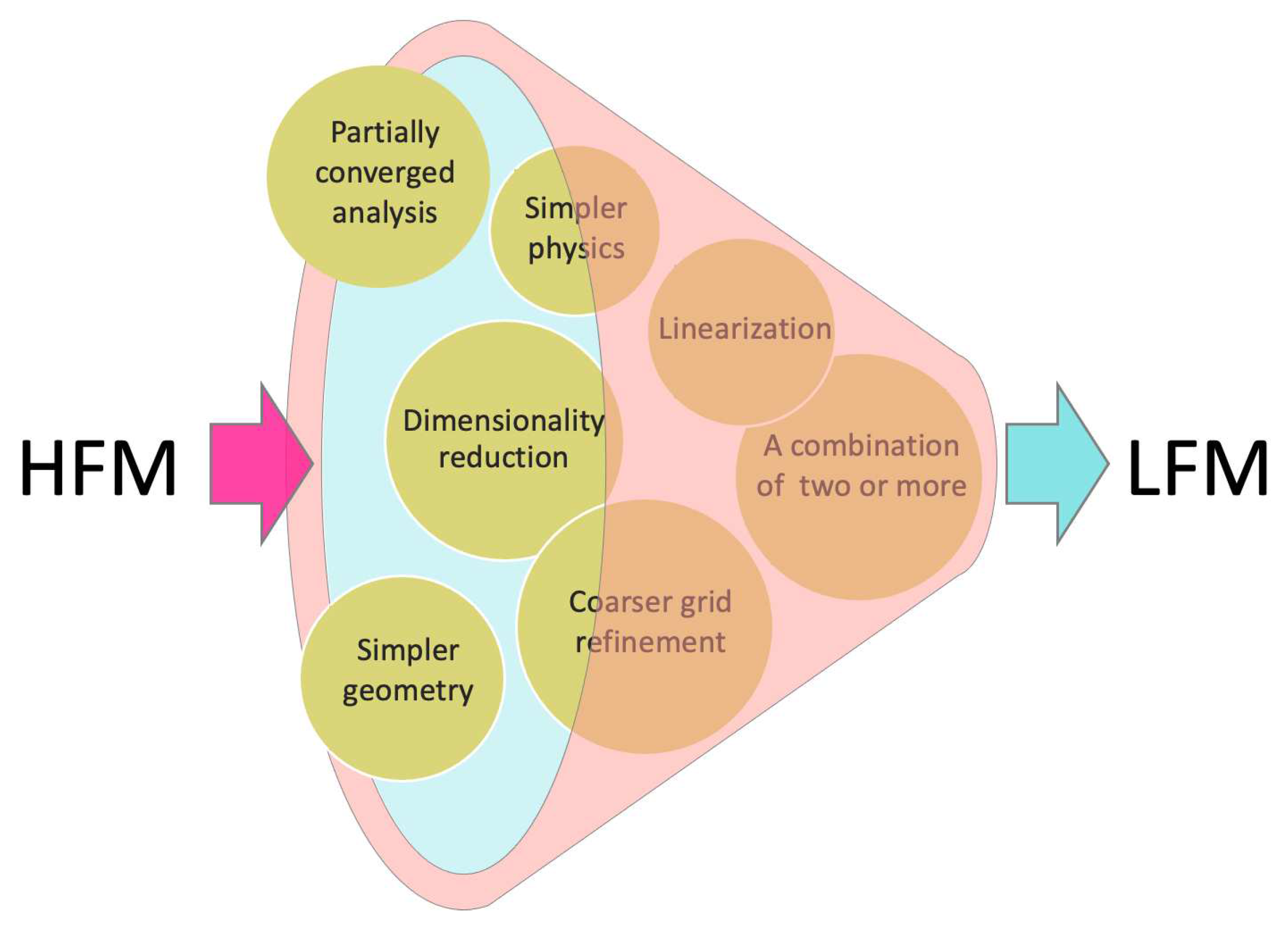
In science and engineering, high-fidelity models (HFMs) commonly refer to complex high-dimensional systems that can make highly accurate predictions. However, the cost of developing and utilizing such models is often prohibitively high, which limits their practicality for many applications. Alternatively, low-fidelity models (LFMs), their simpler and cheaper counterparts, offer a more affordable alternative. LFMs are less accurate due to dimensionality reduction, linearization, use of simpler physics models, coarser domains, or partially converged results, as depicted schematically in
Figure 1. If a model is considered to have low or high fidelity can only be determined relative to another. A fully three-dimensional simulation can be considered expensive compared to an analytical function evaluation but cheap compared to actual experiments. In the early 2000s, multi-fidelity models (MFMs), which combine multiple fidelities in a single model, gained significant attention due to their potential to achieve the desired level of accuracy at a lower cost.
MFMs typically involve the construction of surrogate models (SMs) in order to reduce the computational burden associated with a large number of expensive simulations required for tasks such as optimization (e.g., [
58,
183]) and uncertainty quantification (UQ) (e.g., [
136]). SMs are approximations created to model the behavior of the underlying system. The construction of SM architectures trained using data from different levels of fidelity is referred to as multi-fidelity surrogate modeling (MFSM), which is the primary focus of this review. SMs can also be constructed to reduce the computational cost of individual models. While it is assumed that the reader is familiar with the concept of surrogate modeling,
Appendix B provides a brief overview of the most commonly used surrogate models in the context of MFMs. It should be noted that the choice of the most appropriate SM will depend heavily on the specific characteristics of the problem at hand.
In the framework of computational simulations, the process of fitting an SM to high-fidelity data may be impeded by the computational resources required to obtain just enough data for an accurate approximation. In this scenario, a possible approach to circumvent this issue is to rely on lower-cost, lower-fidelity simulations previously employed to analyze similar problems when computers were less powerful. Alternatively, SMs may be constructed to approximate LFMs, although they may be sufficiently inexpensive to warrant direct usage in some instances. A case in point is illustrated by Nguyen et al., 2013 [
138].
The construction of MFSMs by integrating various fidelity levels is not mandatory for MFMs, as exemplified by Choi et al., 2008 [
36]. In their paper, they employed different fidelity types proficiently through adaptive sampling without constructing an MFSM. This alternative MFM technique is known as MFHM.
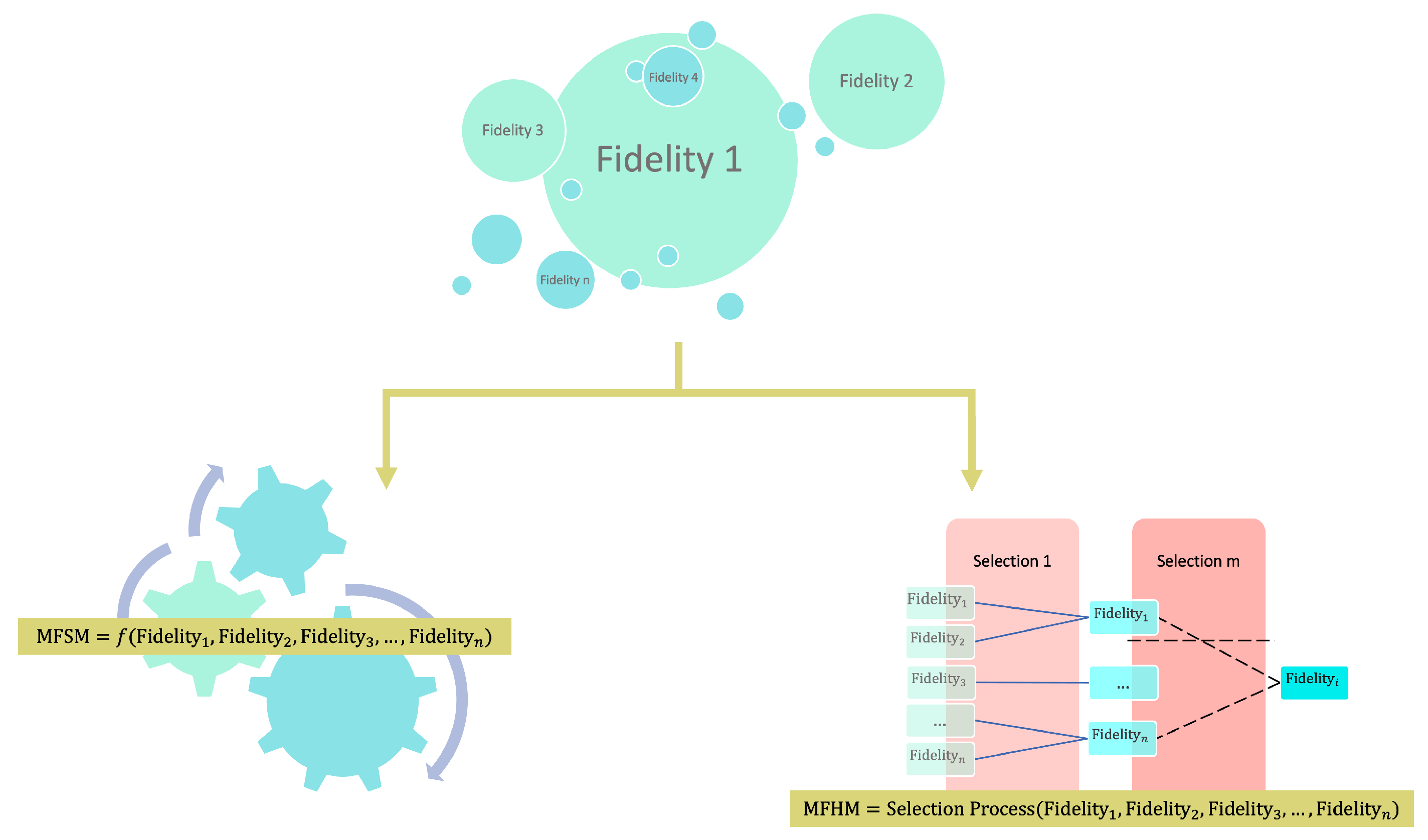
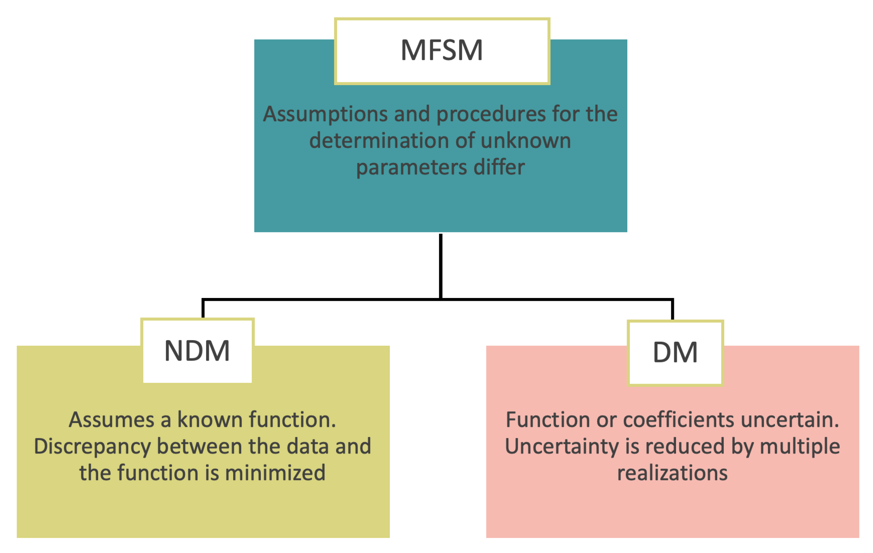
Figure 2 illustrates the options for constructing an MFM. The MFM, where a surrogate model is constructed to combine the fidelities, is termed an MFSM. In contrast, if no surrogate model is built, and the fidelities are combined hierarchically, the resulting technique is known as MFHM. In both techniques, HFMs and LFMs or their surrogate models are utilized.
Most of the articles reviewed in this paper have limited the construction of MFMs to two fidelities. However, it is worth noting that MFMs can be developed using more than two fidelities, as demonstrated in several studies, including Huang et al., 2006 [
76], Forrester et al., 2007 [
58], Qian et al., 2008 [
147], Le Gratiet, 2013 [
109] and Goh et al., 2013 [
66].
Another survey on multi-fidelity modeling is the work of Peherstorfer et al., 2016a [
145]. They focus primarily on methodologies for using MFMs in outer-loop applications, such as optimization, uncertainty propagation, and inference. In contrast, this survey focuses on the penalty and savings associated with combining multiple physics-based models, particularly when these models are fused to create MFSMs. It is worth noting that in this survey, the term multi-fidelity is used only for methods combining at least two physical models. Therefore, articles that consider a physical model and its SM as different fidelities are not seen as MFMs in this review. Methods such as multi-level methods, which replace the HFM with an LFM (with occasional accuracy checks), are not considered as MFMs in this review either. These model reduction methods speed up processes such as optimization at the cost of reduced accuracy. In contrast, MFMs aim to balance accuracy and affordability.
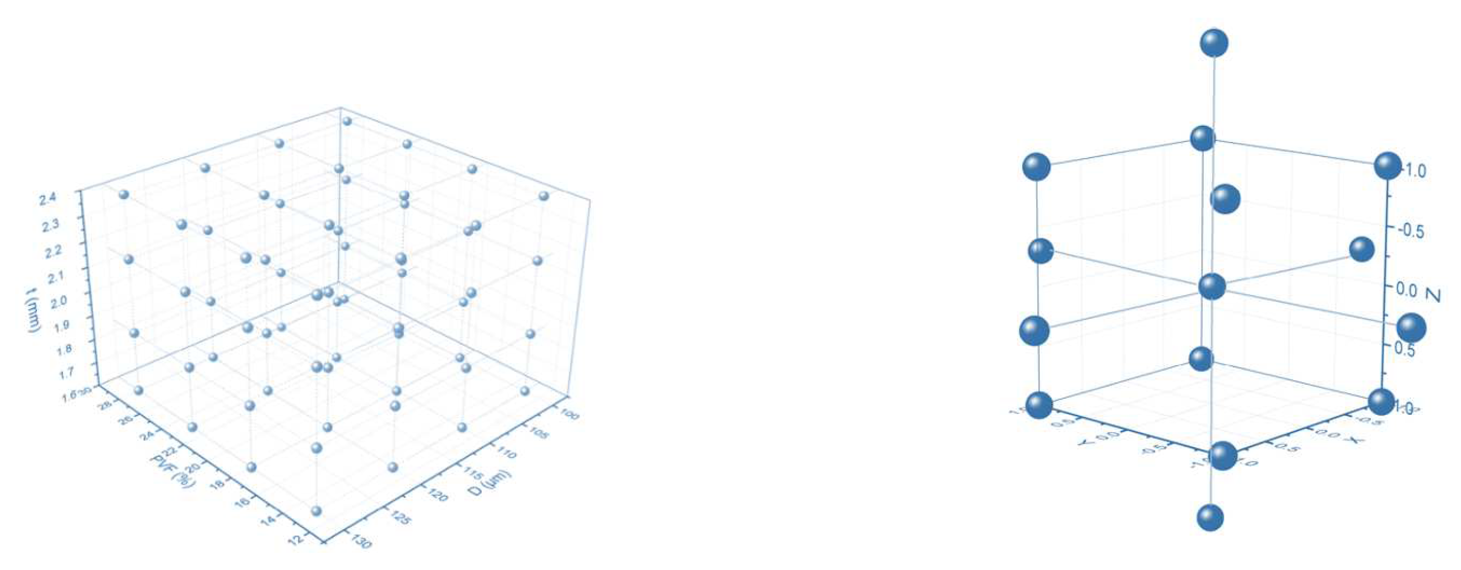
The development of MFM techniques offers the potential to reduce computational costs while maintaining accuracy in various scientific fields. However, it has been noted that the process of developing MFMs requires a significant investment of time and effort by the user and that the point at which the payoff justifies it remains unclear. Hence, one of the goals of this study aims to quantify the efficacy of MFM techniques in maintaining modeling accuracy while reducing its computational cost. This study also aims to comprehensively explore the use of MFMs in scientific research. MFMs will first be introduced, providing information on their field of application, simulation models, year of publication, and fidelity types gathered from the analysis of over 150 papers. The different fidelities utilized in MFMs across scientific fields are categorized. The available techniques for combining fidelities through surrogate models in MFMs are reviewed and evaluated. Sampling strategies used in constructing MFMs are also investigated. Successful combinations of fidelities that significantly improve accuracy and cost through MFMs are identified. Finally, a standard and effective reporting method is suggested to provide readers with a clear understanding of the benefits of MFMs. Papers that have reported such information to facilitate a better understanding of the potential benefits of MFMs are discussed. Overall, this study seeks to contribute to a deeper understanding of the advantages and shortcomings of MFMs in scientific research.
2. Overview
In this study, a comprehensive analysis of various MFM implementations has been carried out, and a classification scheme based on six key attributes has been constructed. The classification categories include application, fidelity type, method for constructing the MFSM (i.e., deterministic method and non-deterministic method), year of publication, paper field, and SM used.
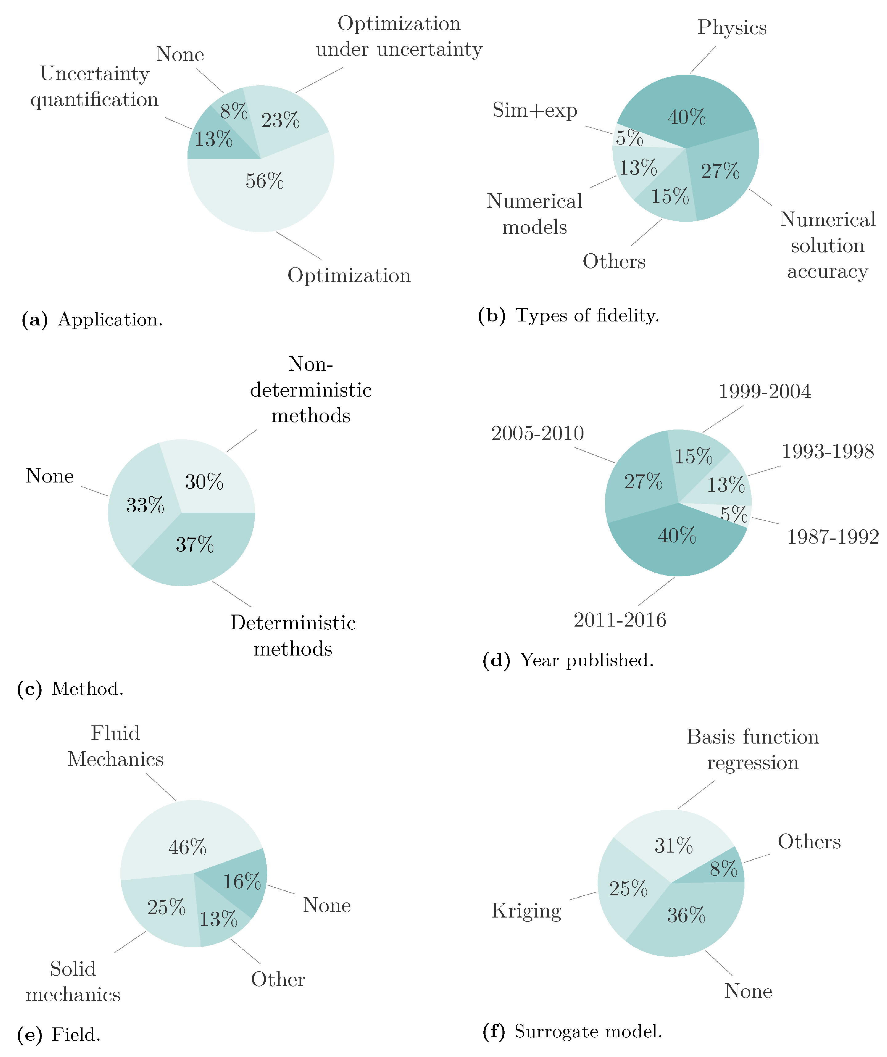
Figure 3 presents an overview of the categories in the reviewed literature.
The reviewed literature focuses on using MFMs in three main applications: optimization (including inference and inverse problems), uncertainty quantification or UQ, and optimization under uncertainty. In cases where papers describe a generic procedure without a specific application, such as analytic functions, they are classified as none. The nature of the fidelities in the model, referred to as the types of fidelity, can be classified into four categories. The first category is physics, which accounts for differences in the assumptions and considerations in the physical model. The second category is numerical solution accuracy, which accounts for different levels of discretization in space or time and partially converged solutions. The third category is numerical models, which refers to instances where the same physical model and assumptions are used, but the method of computing the results varies. Finally, the fourth category is sim+exp, which refers to the combination of simulations, usually as LFM, and experiments, usually as HFM, in constructing an MFM.
The criterion used to fit the data in the MFSM construction is referred to as the method, which can be classified into two categories: deterministic or DM and non-deterministic or NDM. Papers that use MFHMs where no MFSM is constructed are classified as none. The paper’s year of publication is referred to as the year published. The area of application of the problem addressed in the paper is referred to as the field. The most common fields observed in the reviewed literature were fluid mechanics and solid mechanics. Finally, the type of SM used to construct the MFSM is referred to as the surrogate model. Papers that use MFHMs without constructing an MFSM are classified as none.
Figure 3a shows that the most common application found for MFMs is optimization, followed by UQ and optimization under uncertainty. These applications are introduced as outer-loop applications by Peherstorfer et al., 2016a [
145] and extensively discussed in sections 5, 6, and 7 of their work. The fact that optimization is the main application is understandable because UQ and optimization under uncertainty are relatively new subjects. However, it is expected that more publications will appear in these applications.
Figure 3b shows the distribution of papers by the type of fidelities used; these are discussed in
Section 3.
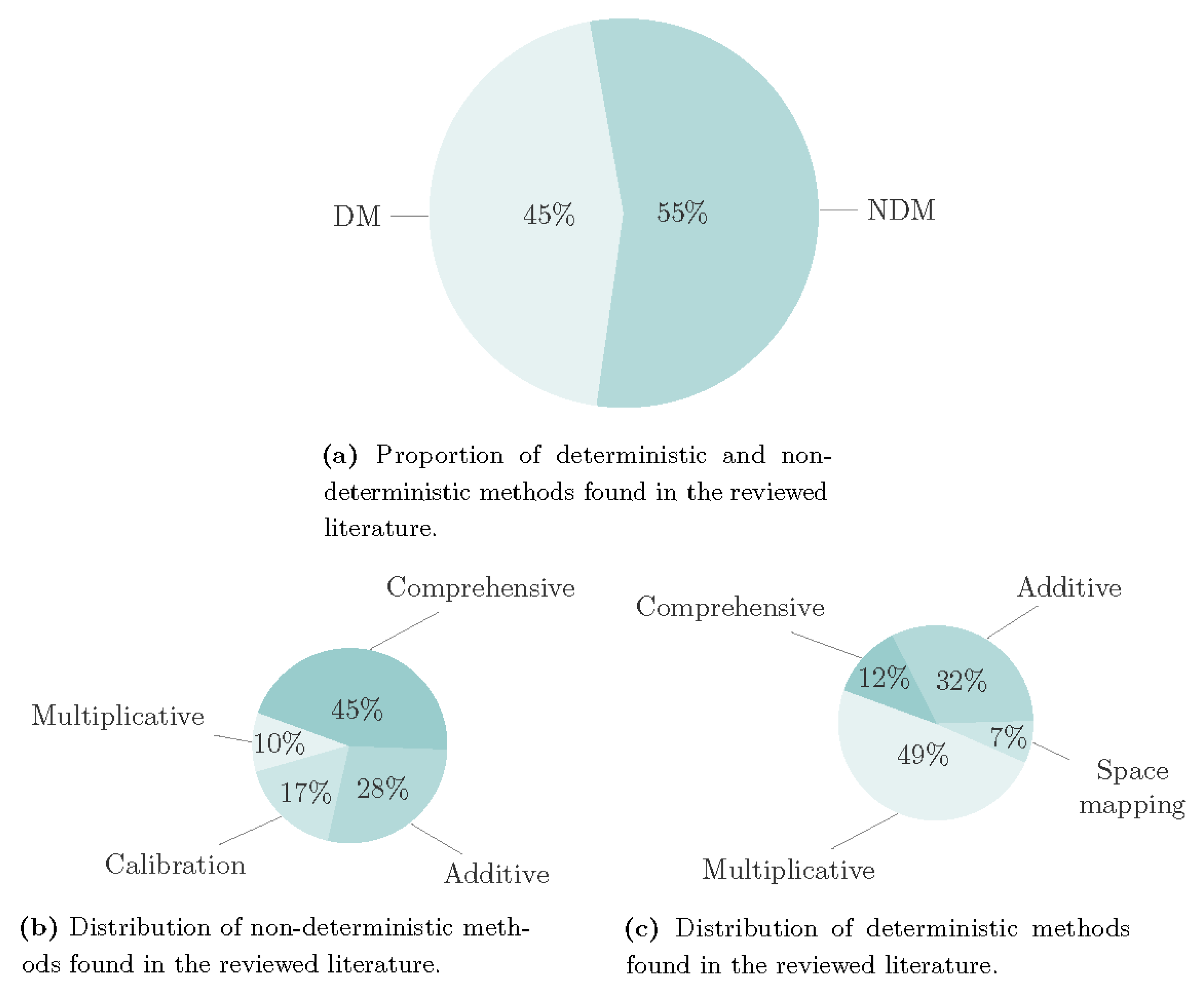
Figure 3c shows that the proportion of papers that use DMs or NDMs to construct an MFSM is similar. The category none refers to papers that present MFMs without constructing an MFSM, called MFHMs. This approach is frequently observed in fields such as optimization, where LFMs are initially utilized to narrow down the domain of interest, followed by the implementation of HFMs to achieve more accurate information about the optimum location, see Rodriguez et al., 2001 [
161] and Peherstorfer et al., 2016b [
144]. The most common methods used to combine fidelities in the MFM context are presented in
Section 4.
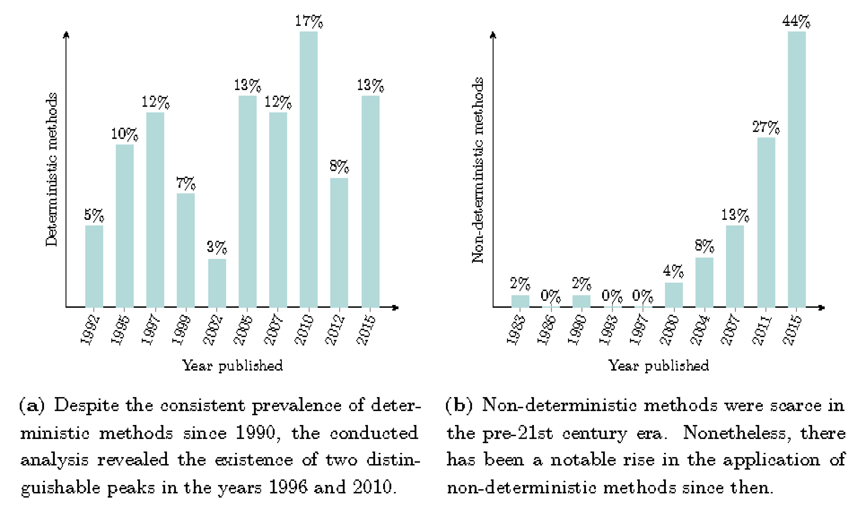
Section 4.3 presents a further study of the time distribution of DMs and NDMs.
Figure 3d shows that the use of MFMs seems to be expanding since its beginning in the late ’80s. Finally, the distribution of MFMs applications across various fields is presented in
Figure 3e. It indicates that most of the reviewed papers implement MFMs in fluid mechanics and solid mechanics. However, other fields, such as electronics, aeroelasticity, and thermodynamics, also feature in the reviewed literature. Furthermore, some papers do not have any specific application, but rather use mathematical functions like Hartman or Rosenbrock to test the methods.
Figure 3f displays the distribution of papers by surrogate type used for constructing MFSMs. The study found that basis function regression and Kriging surrogates are the two most commonly used types for constructing an MFSM. The category
others includes artificial neural networks, moving least squares, support vector machines, radial basis interpolation, and proper orthogonal decomposition, each with a usage of less than 1%. In addition, the research reveals that some MFMs do not require the construction of an MFSM, referred to as MFHM, which is included in the category
none. For instance, Choi et al., 2008 [
36] proposes a hierarchical MFM approach for optimization, utilizing HFMs selectively to rectify inadequacies of LFMs. As mentioned, this technique does not involve constructing MFSMs or explicitly integrating fidelities. Other examples are Kalivarapu and Winer, 2008 [
84], where an MFM is used for interactive modeling of advective and diffusive contaminant transport with no MFSM construction. Giunta et al., 1995 [
64], and Zahir et al., 2013 [
199] are other examples of such cases.
Section 5 provides a detailed analysis of the computational cost and accuracy associated with using MFMs. Additionally, it offers guidelines for authors on how to present cost savings and accuracy improvements. Sampling methods used for MFSM construction are discussed in
Appendix A, while
Appendix B introduces the most commonly used surrogate methods in MFSM research.
3. Types of Fidelity
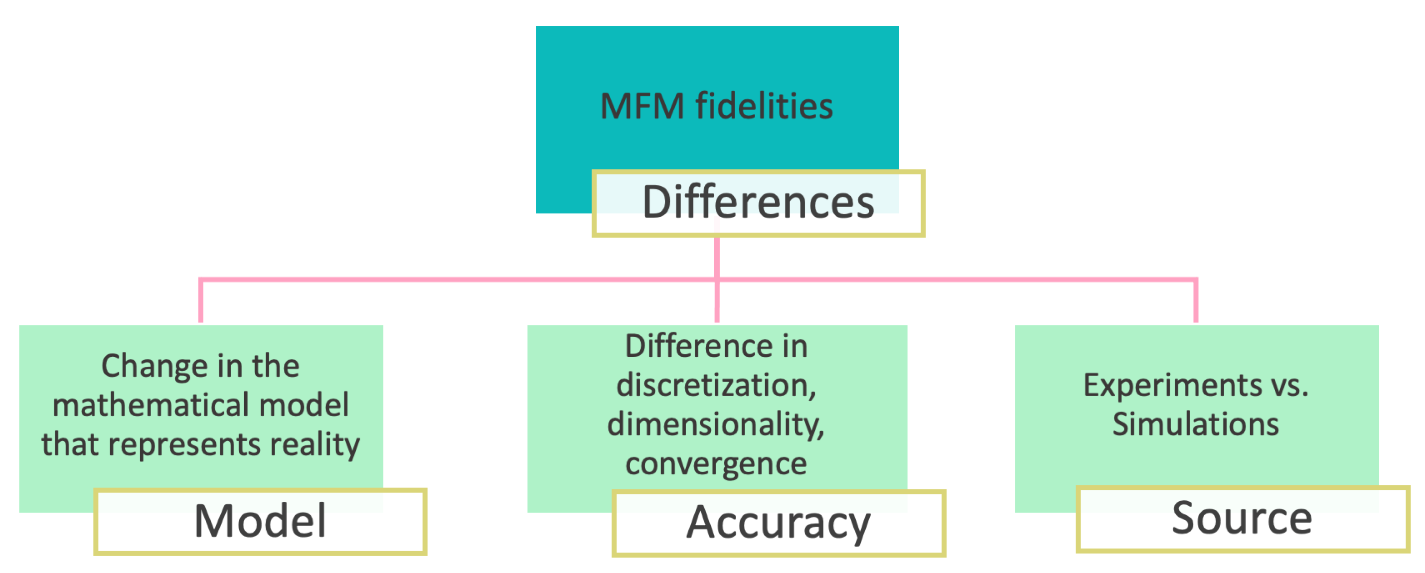
The current study aimed to review the literature and identify different types of fidelities commonly associated with three principal categories:
model,
accuracy and
source (
Figure 4). Model involves simplifying the mathematical representation of the physical phenomenon, typically by simplifying the differential equations being solved or the numerical model. Accuracy refers to changes on the discretization of the model, such as using smaller grid elements or shorter time steps for HFMs. Source is associated with the incorporation of experimental results in addition to simulations, which are regarded as having the highest level of fidelity.
Authors may explicitly state the superiority of one fidelity over another, as in the scenario involving a refined grid as opposed to a coarser grid if the same model is used. Nevertheless, in cases such as comparing a one-dimensional model with a refined grid against a three-dimensional model with a coarser grid, the comparative superiority of fidelities may not be apparent. Peherstorfer et al., 2016a [
145] classified LFMs in three categories:
simplified models,
data-fit models, and
projection-based models. Their simplified models’ category includes the differences between fidelities discussed in this study. In contrast, data-fit models and projection-based models are included in this review as surrogate modeling techniques in
Appendix B.
This survey identified two main fields where MFMs are used, fluid mechanics and solid mechanics. In fluid mechanics, the primary fidelity types were
analytical expressions,
empirical relations,
numerical linear approximations,
potential flow,
numerical non-linear non-viscous approximations (Euler),
numerical non-linear viscous approximations (RANS),
coarse vs. refined analysis, and
simulations vs. experiments. A detailed listing of the papers that employed these types of fidelities as LFMs and HFMs is provided in
Table 1.
Other types of fidelities, that were not included in the table, were found in the literature. These included simplifying physics found in Castro et al., 2006 [
29], where an earth penetrator problem is simplified by assuming a rigid penetrator and in Goldfeld et al., 2005 [
67], where the physics are simplified by assuming constant instead of variable material properties; using different geometries in Forrester et al., 2010 [
56], where the LFM is a RANS simulation with simplified geometry and the HFM is a RANS simulation with full geometry; and using different numbers of Monte Carlo samples in Keane, 2012 [
88]. In fluid mechanics, additional categories were also found including dimensionality (e.g., 2D/3D), coarse vs. refined analysis, simulations vs. experiments, transient vs. steady, and semiconverged vs. converged solutions (
Table 2).
Several types of fidelities were identified in the literature but not included in
Table 2. For instance, Castro et al., 2006 [
29] simplified a physics problem by assuming a rigid penetrator, while Goldfeld et al., 2005 [
67] simplified the physics by assuming constant material properties instead of variable ones. Forrester et al., 2010 [
56] used RANS simulations with simplified and complete geometries for the LFM and HFM, respectively. Additionally, Keane, 2012 [
88] varied the number of Monte Carlo samples used. In the field of fluid mechanics, various additional fidelity categories were also found, such as dimensionality, level of analysis refinement, simulation versus experimentation, transient versus steady states, and semiconverged versus fully converged solutions.
Table 2 presents a detailed summary of these categories.
Table 3 presents the common types of fidelities employed in the domain of solid mechanics. These types comprise of
mesh density,
material models, and
temperature. However, the investigation revealed other fidelity types that were not included in
Table 3. For example, Kim et al., 2007 [
91] employed
isothermal and
non-isothermal analyses for LFM and HFM, respectively. In addition to these, several more categories of fidelities were discovered in solid mechanics, such as
dimensionality (e.g., 2D/3D),
coarse vs. refined,
simulations vs. experiments, and
boundary condition simplification (e.g., infinite plate vs. finite plate), and are presented in
Table 4.
In addition, papers from other fields such as electronics and robotics, and papers based on analytical functions were reviewed. In electronics, the most common method utilized was coarse vs. refined analysis, although some papers, such as Absi and Mahadevan, 2016 [
1], employed steady vs. transient models. In robotics, Winner et al., 2000 [
192], determined the fidelities based on the complexity of the robot’s resources. Several academic papers have utilized mathematical functions to examine the effectiveness of different methods, including analytical function versus analytical approximations of the function. These studies include the works of Robinson et al., 2006 [
157][
159], Zimmermann and Han, 2010 [
206], Ng et al., 2012 [
136], Le Gratiet, 2013 [
110], Raissi and Seshaiyer, 2013 [
149], Raissi and Seshaiyer, 2014 [
150], and Goh et al., 2013 [
66]. Lastly, the category of methods for uncertainty analyses with no particular application, includes Burton and Hajela, 2003 [
28], Eldred, 2009 [
50], Perdikaris et al., 2015 [
146], Peherstorfer et al., 2016b [
144], and Chaudhuri and Willcox, 2016 [
32]. In Burton and Hajela, 2003, Eldred, 2009, and Perdikaris et al., 2015, the types of fidelity pertained to less and more accurate uncertainty analysis. Peherstorfer et al., 2016b [
144] utilized LF models to aid in the construction of the biasing distribution for importance sampling and a small number of HF samples to obtain an unbiased estimate. Chaudhuri and Willcox, 2016 [
32], employed an iterative method that used low-fidelity surrogate models (LFSMs) to estimate coupling variables and adaptively sampled the HF system to enhance the SM, while retaining a comparable level of precision in uncertainty analysis as the fully coupled HF multidisciplinary system.
Figure 1.
Connection between high-fidelity and low-fidelity models is commonly observed to be attributed to one or more of the following factors: Dimensionality reduction, grid coarsening, linearization, partial convergence, reduced complexity in geometry, and simplified physics.
Figure 1.
Connection between high-fidelity and low-fidelity models is commonly observed to be attributed to one or more of the following factors: Dimensionality reduction, grid coarsening, linearization, partial convergence, reduced complexity in geometry, and simplified physics.
Figure 2.
Within the frame of multi-fidelity modeling, surrogate models are commonly used to integrate information from different fidelities. When constructing a surrogate model that combines fidelities explicitly, such as co-Kriging, the resulting approach is referred to as a multi-fidelity surrogate model. In contrast, multi-fidelity hierarchical models combine fidelities without requiring an explicit multi-fidelity surrogate model architecture. Methods such as importance sampling fall under the multi-fidelity hierarchical category.
Figure 3.
Proportion of different attributes considered in the multi-fidelity model papers reviewed, the charts are based on 157 papers.
Figure 3.
Proportion of different attributes considered in the multi-fidelity model papers reviewed, the charts are based on 157 papers.
Figure 4.
Main differences between fidelities found in the literature.
Figure 4.
Main differences between fidelities found in the literature.
Figure 5.
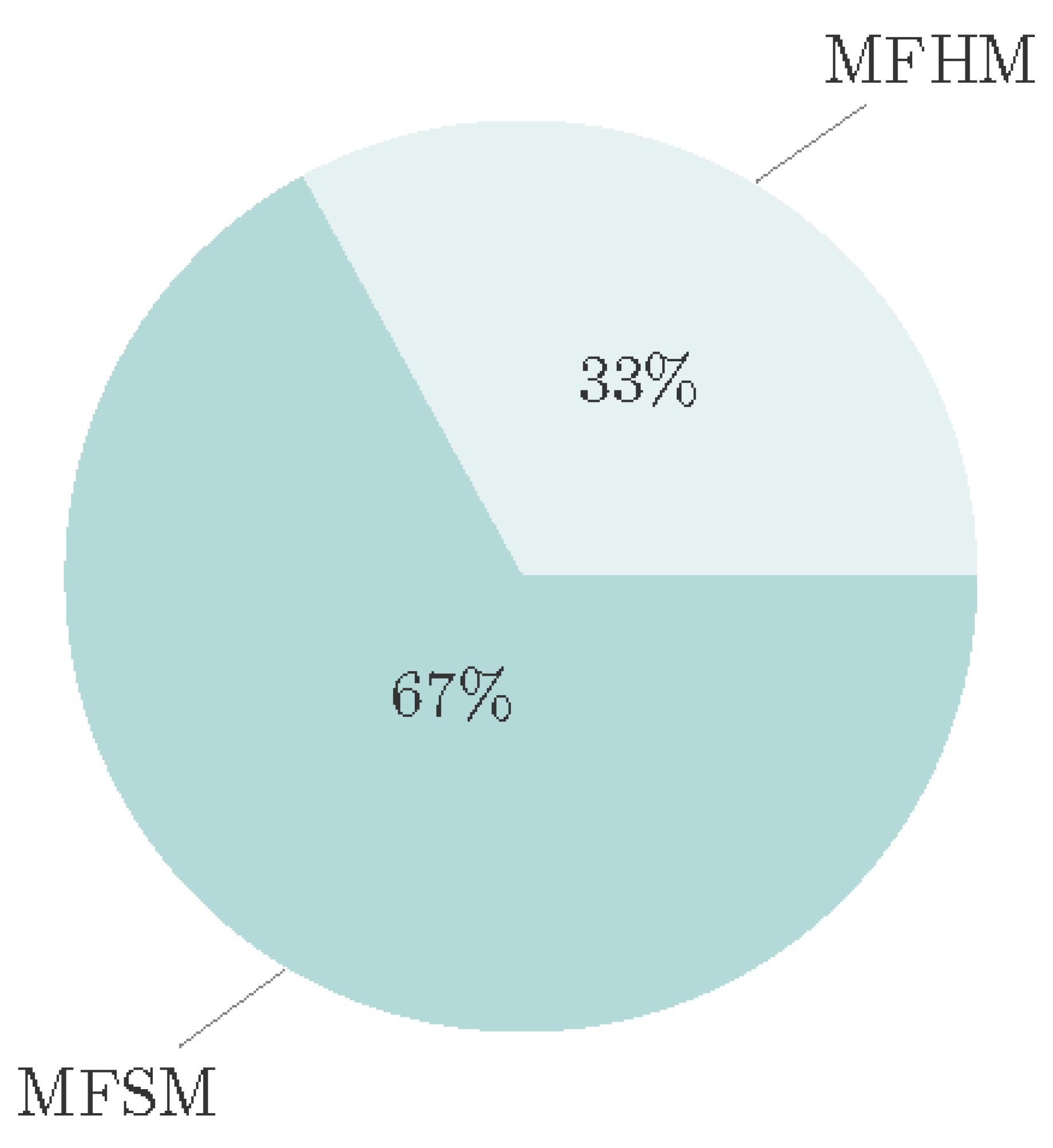
Among the 157 papers that were scrutinized, a total of 105 studies were found to have developed a multi-fidelity surrogate model that explicitly integrates the different levels of fidelities. The remaining papers, however, have introduced multi-fidelity hierarchical models.
Figure 5.
Among the 157 papers that were scrutinized, a total of 105 studies were found to have developed a multi-fidelity surrogate model that explicitly integrates the different levels of fidelities. The remaining papers, however, have introduced multi-fidelity hierarchical models.
Figure 6.
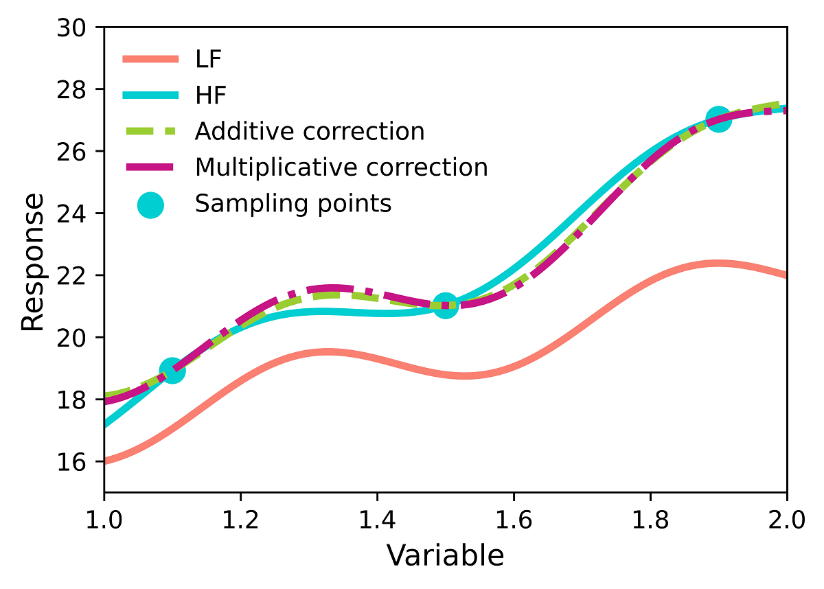
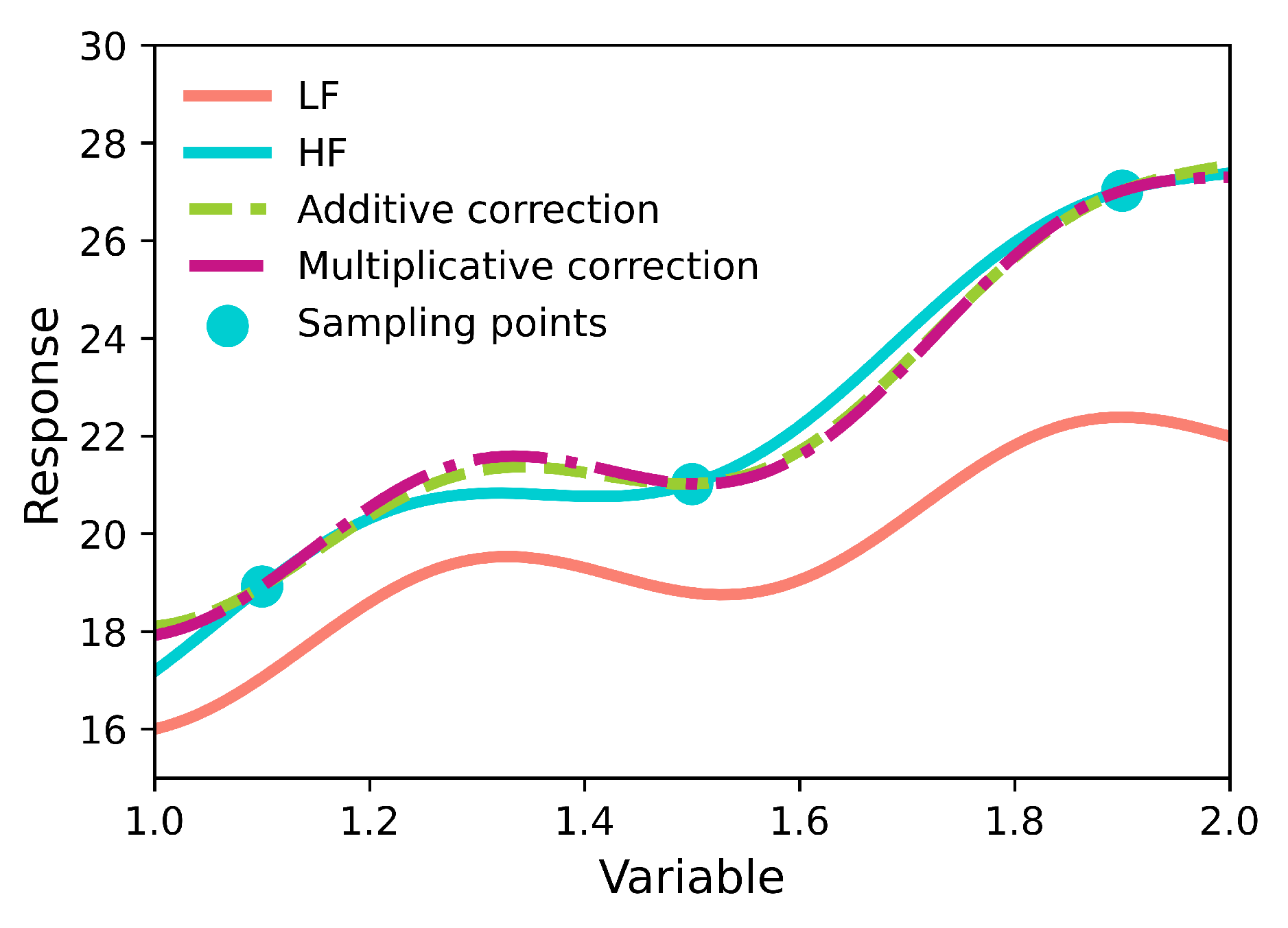
One-dimensional, analytic example that illustrates the performance of additive and multiplicative corrections.
Figure 6.
One-dimensional, analytic example that illustrates the performance of additive and multiplicative corrections.
Figure 7.
Multi-fidelity surrogate models’ parameters are inferred utilizing either deterministic or non-deterministic methodologies contingent upon the underlying presumptions of the unknown parameters.
Figure 7.
Multi-fidelity surrogate models’ parameters are inferred utilizing either deterministic or non-deterministic methodologies contingent upon the underlying presumptions of the unknown parameters.
Figure 8.
Proportion of deterministic and non-deterministic methods utilized for the construction of multi-fidelity surrogate models based on the literature. The chart also displays the distribution of the combination methods introduced in
Section 4.2 within each category, deterministic and non-deterministic methods.
Figure 9.
Frequency of publication over time for both deterministic and non-deterministic methods.
Figure 9.
Frequency of publication over time for both deterministic and non-deterministic methods.
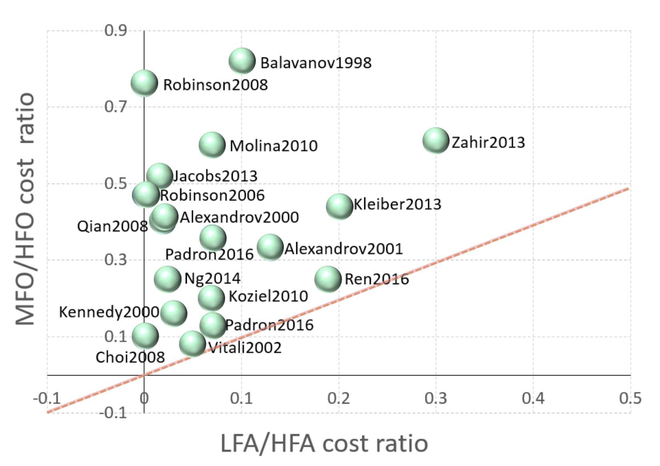
Figure 10.
Cost ratio between a single analysis of the low-fidelity model and a single analysis of the high-fidelity model (LFA/HFA cost ratio) vs. cost ratio between the optimization process using an MFSM and the optimization process using an HFM (MFO/HFO cost ratio). The dashed line is the threshold line, below which the points indicate no speed ups from using multi-fidelity models.
Table 1.
Categorization of fluid mechanics-focused papers based on the methodologies employed as high- and low-fidelity models. The analysis techniques used in these studies were analyzed and categorized into six distinct categories: analytical approach (An), empirical methods (Em), linear analysis (Li), potential flow models (PF), Euler analysis (Eu), and Reynolds-averaged Navier-Stokes techniques (RANS).
Table 2.
Distinct types of fidelity implemented in research papers on fluid mechanics, which differ from those based on analysis type. The classifications include dimensionality (2D/3D), analysis resolution (coarse vs. refined), type of study (simulations vs. experiments), state of flow (transient vs. steady), and degree of solution convergence (semiconverged vs. converged). Each paper’s physical model is designated by the following abbreviations: Em (empirical), Li (linear), PF (potential flow), Eu (Euler), RANS (Reynolds-averaged Navier-Stokes), URANS (unsteady RANS), TM (turbulence method), MHD (magnetohydrodynamics), AE (aeroelastic equations), MPF (multiphase flow), and TM (thermomechanical equations).
| Fluid mechanics |
|---|
| Fidelity type |
Reference |
| Dimensionality |
[57] 2D/3D Eu, [82] 1D/3D RANS+TM, [85] 2D/3D URANS, [108] 2D/3D, [147] 1D/2D RANS, [158] 1D/2D Li, [178] 1D/3D RANS, [190] 1D/3D RANS, [207] 1D,2D/3D RANS |
| Coarse/Refined |
[5] Eu, [25] RANS, [34] Eu, [35] Eu, [36] Li/Eu, [83] RANS, [89] MPF, [92] MHD, [99] Eu, [100], Eu[103] Eu, [116] Eu, [120] RANS, [155] RANS, [173] RANS, [199] Eu/RANS |
| Exp./Sim. |
[53] Euler/MHD, [56] PF/Em, [105] RANS, [174] RANS |
| Semiconverged/Converged |
[83], RANS[100] Eu |
| Steady/Transient |
[20] AE, [62] Eu, [173] TM |
Table 3.
Categorization of papers within the domain of solid mechanics, according to the fidelity type employed in their analyses. The four fidelity types included are: analytical (An), empirical (Em), linear (Li), and non-linear (NL).
Table 3.
Categorization of papers within the domain of solid mechanics, according to the fidelity type employed in their analyses. The four fidelity types included are: analytical (An), empirical (Em), linear (Li), and non-linear (NL).
Table 4.
Categorization of solid mechanics research papers according to the type of fidelity used. The fidelity categories are defined based on dimensionality (i.e., 2D/3D), degree of refinement (i.e., coarse vs. refined), and simplification of boundary conditions (i.e., infinite plate vs. finite plate). Each paper is associated with the corresponding model employed, with Li indicating the use of linear models and NL representing non-linear models.
| Solid mechanics |
|---|
| Fidelity type |
Reference |
| Dimensionality |
[111] 1D/2D Li, [113] 1D/3D, [124] 2D/3D, [125] 2D/3D Li, [166] 2D/3D Li, [168] 2D/3D NL |
| Coarse/Refined |
[12] Li, [21] NL, [23] Li, [24] NL, [31] Li, [114] Li, [123] Li, [169] NL, [170] NL, [189] Li, [197] Li, [198] Li |
| Boundary conditions |
[185] Li, [188] Li |
Table 5.
Papers that use deterministic methods for the construction of multi-fidelity surrogate models.
Table 5.
Papers that use deterministic methods for the construction of multi-fidelity surrogate models.
Table 6.
Papers that use non-deterministic methods to construct multi-fidelity surrogate models.
Table 6.
Papers that use non-deterministic methods to construct multi-fidelity surrogate models.
Table 7.
MFM/HFM cost ratio. The references are divided also per field, given by fluid mechanics, solid mechanics and other. Other includes electronics, aeroelasticity, thermodynamics and analytical functions.
Table 7.
MFM/HFM cost ratio. The references are divided also per field, given by fluid mechanics, solid mechanics and other. Other includes electronics, aeroelasticity, thermodynamics and analytical functions.
Table 8.
Padrón et al., 2016 [
140] cost, savings and accuracy report as a model for authors.
Table 8.
Padrón et al., 2016 [
140] cost, savings and accuracy report as a model for authors.
| Property |
Value |
a Comments |
| Cost LF/HF |
0.07 |
a LF= Euler, HF= RANS |
| Error LF/HF |
0.18 |
- |
| Cost MF/HF |
0.13 |
a MF= 1 HF + 17 LF |
| Error MF/HF |
0.05 |
- |
