
Submitted:
01 May 2023
Posted:
02 May 2023
You are already at the latest version
Abstract
Through the use of machine learning algorithms like the Support Vector Machine, it has been show that burn extent can be accurately mapped from hyperspatial drone imagery in both grasslands and forests. Despite these successes, hyperspatial imagery must be acquired via drones, requiring large amounts of time and resources to capture areas much smaller than the large catastrophic fires which result in the majority of the lands burned each year by wildland fires. To overcome this difficulty, high spatial resolution satellite imagery from Worldview2 can be substituted for hyperspatial drone imagery, allowing for larger regions of images to be acquired more easily and efficiently. Additionally, Worldview2 trades spatial resolution for spectral resolution and extent, capturing images in 8 multispectral bands as opposed to 3 band imagery in the visible spectra. This research examines the utility of each of the 8 bands observed in Worldview2 imagery using an Iterative Dichotomiser 3 decision tree, then uses these bands to map burn extent and biomass consumption. Several classifications of burn extent and biomass consumption are produced and compared based on the bands used as inputs. The results show that using Worldview2 imagery to map burn extent and biomass consumption results in highly accurate maps, with slight improvements when additional bands are added.
Keywords:
Support Vector Machine (SVM)
; Worldview2
; Satellite Imagery
; Iterative Dichotomiser 3 (ID3)
; Burn Extent
; Burn Severity
; Biomass Consumption
1. Introduction
This project explores the mapping of burn extent and severity from very high-resolution satellite imagery using a Support Vector Machine (SVM) performing pixel-based classifications. Post-fire Worldview2 imagery of the Mesa Fire near Council, Idaho, USA was acquired from September 2018, made available for university researchers through the Commercial Smallsat Data Acquisition (CSDA) program [1]. Through the use of very high-resolution satellite imagery such as Worldview2, this project explores the feasibility of mapping burn extent as well as biomass consumption, which is a measure of burn severity. Additionally, the analysis explores the utility of the individual bands when used by the SVM for mapping burn extent and severity.
A century of fire suppression in the western US has resulted in a departure from fire return intervals experienced under pre-European settlement conditions. This has resulted in a significant increase in large catastrophic high severity fires since 2000 [2]. Nineteen of the twenty worst fire seasons in the US have been experienced in this century, with some fire seasons resulting in more than four million hectares burned with suppression costs exceeding four billion dollars annually. Interestingly, there has actually been a reduction in the quantity of fires during the same period [3], [4].
These large catastrophic fires result in increased post-fire erosion, degraded wildlife habitat and loss of timber resources. This loss results in negative impacts on ecosystem resilience as well as increased risk to communities in the wildland-urban interface. Wildland fires claim more lives in the US than any other natural disaster, with an average loss of 18 wildland fire fighters per year [5], [6]. The 2018 Camp Fire in northern California resulted in 85 fatalities and uninsured losses in excess of ten billion dollars, leading the list of the top ten fires most destructive to human development, nine of which have occurred since 2000 [7].
Effective management of wildland fire is essential for maintaining resilient wildlands. Actionable knowledge of the relationship between fire fuels, fire behavior and the effects of fire on ecosystems as well as human development can enable wildland managers to deploy innovative methods for mitigating the adverse impacts of wildland fire [8]. The knowledge extracted from remotely sensed data enable land managers to better understand the impact wildfire has had on the landscape, providing an opportunity for better management actions resulting in improved ecosystem resiliency.
Background
Local fire managers are overwhelmed by the severity of wildland fires, lacking the resources to make informed decisions in an adequate measure of time. Regulations within the United States require fire recovery teams to acquire post-fire data within 14 days of containment, including the mapping of burn extent [9]. Currently, fire managers and recovery teams have been using Landsat imagery, which contains 8 bands of 30m spatial resolution along with a panchromatic band (15m) and two thermal bands (100m) [10]. Assuming that there are no clouds or smoke obstructing the view of the fire, Landsat imagery can only be collected for a site once every 16 days, making it difficult to acquire data within the time required.
Burn Severity and Extent
The term “wildland fire severity” can refer to many different effects observed through a fire cycle, from how intense an active fire is burning, to the response of the ecosystem to the fire over the subsequent years. This study investigates direct or immediate effects of a fire such as biomass consumption as observed in the days and weeks after the fire is contained [11]. Therefore, this study defines burn severity as the measurement of biomass (or fuel) consumption [12].
Identification of burned area extent within an image can be achieved by exploiting the spectral separability between burned organic material (black ash and white ash) and unburned vegetation [13], [14]. Classifying burn severity can be achieved by separating pixels with black ash (low fuel consumption) from white ash (more complete fuel consumption), relying on the distinct spectral signatures between the two types of ash [15]. In forested biomes, low severity fires can also be identified by looking for patches of unburned vegetation within the extent of the fire. If a patch is comprised only of tree crowns, the analysis can infer that the vegetation is a tree which the fire passed under, and classify the pixels as low intensity surface fire [16]. If the patch of vegetation contains herbaceous or brush species, then the patch is actually an unburned island within the burned area and can be classified as unburned [17].
Support Vector Machine
The Support Vector Machine (SVM) is a pixel-based classifier that can be used to label or classify pixels based on an image pixel’s band values. The data used to train the SVM consists of manually labeled regions of pixels that have the same class label, such as would be encountered when labeling post-fire effects classes such as “burned” or “unburned”. When training the classifier, the SVM creates a hyperplane inside the multi-dimensional band decision space, dividing the decision space between training classes based on their pixel band values. When classifying the image, pixels are classified based upon which side of the hyperplane a pixel lands when placed in the decision space based on the pixel’s band values [18].
The SVM has been used in the past to determine the burn extent of a fire, however, hyperspatial drone imagery was used instead of high-resolution satellite imagery. Hamilton [19] found that when using hyperspatial drone imagery with a spatial resolution of five centimeters, the SVM classified burn extent with 96 percent accuracy. Zammit [20] also utilized an SVM to perform a pixel-based burned area mapping from the green, red and near-infrared (NIR) bands from 10 meter resolution imagery acquired with the SPOT 5 satellite. Likewise, Petropoulos [21] used an SVM to map burn extent from the visible and near infrared ASTER bands with 15 meter resolution. Both Zammit and Petropoulos obtained accuracy slightly lower than observed by Hamilton.
Despite the success Hamilton [19] had mapping burn extent and severity using hyperspatial drone imagery, the possibility of using high-resolution satellite imagery has even greater implications. The Worldview-2 satellite was launched in 2009 with the ability to generate imagery with eight bands ranging from 400 to 1040 nm [22]. The Worldview-2 satellite can map nearly one million square kilometers per day and can revisit an area in less than 27 hours with an orbit of fewer than two hours [23]. Even at an altitude of 770 km, its imagery’s spatial resolution manages to achieve 1.8 meters at nadir or 2.4 meters 20 degrees off-nadir. All these characteristics of Worldview-2 give it the flexibility to aid researchers in mapping burn extent within the previously referenced 14-day window mandated for completion of burn recovery plans.
Entropy Analysis of Image Bands
Hamilton [13] utilized an Iterative Dichotomiser (ID3) [24] to build a decision tree and report the information gain of each attribute from the red, green and blue bands in the color image as well as texture. Information gain facilitated feature engineering, identifying the most effective texture metric for machine learning based mapping of burn extent and severity, where severity was evidenced by the existence of white versus black ash . By reporting on information gain, it was possible to observe the strength of an attribute’s ability to accurately split the training data based on the user designated labels as based on the information content of the training data in relation to that attribute [18]. In order to train the ID3, training regions were designated for black ash, white ash and unburned vegetation on imagery from multiple wildland fires. Once the decision tree was constructed, the attributes with the most information gain will be represented in nodes higher in the tree (closer to the root), while features with less information gain will appear lower in the tree (closer to the leaves).
2. Materials and Methods
This section will describe how high-resolution satellite imagery was used to map burn extent and biomass consumption through machine learning algorithms such as the Support Vector Machine (SVM).
2.1. Data Acquisition
DigitalGlobe’s WorldView2 satellite imagery is commercial imagery but is available to university researchers through the National Aeronautics and Space Administration’s (NASA) Commercial Smallsat Data Acquisition (CSDA) program. DigitalGlobe and NASA partner to offer a NextView license, which temporarily grants users access to DigitalGlobe’s satellite products [1]. With this license, a data request was submitted to cad4nasa.gsfc.nasa.gov that provided bounding coordinates for our area of interest (AOI), the Mesa Fire near Council, Idaho. We were provided with eleven images from multiple satellites that covered our AOI but narrowed the selection down to the best two images, both from the WorldView2 satellite. These images were taken after the Mesa Fire occurred and had minimal cloud cover. The Mesa Fire was chosen for this research because of its size and overlap with hyperspatial imagery acquired by the research team through the use of unmanned aircraft systems (UAS) while assisting researchers from the United States Forest Service Rocky Mountain Research Station in conducting post-fire field studies. While the Mesa Fire covered more than 15,000 hectares, a subsection of imagery that covers roughly 350 hectares was also acquired using drones, which was used as the Area of Interest for this research. Both of these regions can be observed in Figure 1, showing the location of Mesa Fire, as well as the Area of Interest - the region of hyperspatial drone imagery acquired by NNU where Worldview2 imagery was also acquired.
2.2. Training Data
Once Worldview2 imagery was acquired for the Mesa fire, training data was created to map two types of post-fire effects: burn extent and biomass consumption. This process was completed in ArcGIS Pro by using the Training Samples Manager within the Image Classification toolset [25]. The training data used to map post-fire effects contained four classes: black ash, white ash, unburned greenery, and unburned surface. Polygons in the black ash class contain burned areas that experienced low severity burn and resulted in black ash, whereas polygons in the white ash class contain burned areas that experienced high severity burn and resulted in white ash. These classes can be used to map biomass consumption or can be generalized/reclassified to one burned class for mapping burn extent. In addition to mapping burned areas, the SVM classifier also maps all unburned areas in the map, requiring an unburned class. Within the unburned class, two subclasses were included in the training data – unburned greenery and unburned surface. Areas within the unburned greenery polygons include surface vegetation and canopy cover, whereas the areas within the unburned surface polygons contain all other surface area that was not burned, canopy, or vegetation, such as bare dirt, rocks, and roads.
While two classes were created to represent the unburned area, this was only done to increase the accuracy of the burn extent and biomass consumption classifications. Since an SVM can only perform binary classification between two classes, it can be difficult to find/calculate/determine the hyperplane that separates pixels into burned and unburned classes. For example, within the burned class includes areas that contain black ash (very low RGB pixel values) and white ash (very high RGB pixel values), whereas the unburned class contains areas that contain an assortment of regions and RGB pixel values. For these reasons, four classes were created, utilizing multiple SVMs to perform multiclass classification, as opposed to more simple binary classification between two classes. Mapping all four classes, then reclassifying/generalizing to the burn extent classes (burned vs unburned) or biomass consumption (white ash vs black ash) improves the accuracy of each of map by including additional hyperplanes into the decision space, separating the pixels into their appropriate classes with more accuracy, improving the accuracy of the model and classifier.
Once completed, the training data was exported as a .csv, which was used as input when training an Iterative Dichotomizer 3 (ID3) decision tree algorithm. Construction of the decision tree entails selection of the bands that contain the highest information content [26]. This .csv file contained a list of possible attributes and labels, as well as the average band values for each polygon. Additionally, each training dataset was saved in ArcGIS Pro as a shapefile, to be used later for classification with the Support Vector Machine.
2.3. Band Evaluation and Selection Process
The training data tuples exported from ArcGIS Pro were fed into an Iterative Dichotomiser 3 to determine which bands contained the highest information content for mapping burn severity. The training data consisted of a total of 80 training tuples, 20 for each of the four classes. Using an iterative dichotomiser 3 (ID3), coded in C# built using the Windows Presentation Foundation framework, the set of 80 training tuples was divided into subsets until all tuples in the subset could be assigned the same class label, creating a decision tree.
The decision tree is created by selecting the band with the most information as the root and the remainder of the tree is constructed based on which remaining bands contain the most information for classifying the rest of the tuples. As such, any bands that contributed to informing the classification of the tuples were extracted from the imagery to create a new raster Some machine learning algorithms, such as the MR-CNN and implementations of the SVM, are limited to ingesting only 3 bands of imagery, so if the tree contained more than two levels, only the root, and the first two children would be used as extracted to create a new raster.
Additionally, Principal Component Analysis was implemented to reduce the number of dimensions. Since Worldview2 imagery contains 8 bands of images, but some image classification algorithms such as the MR-CNN can only intake 3 bands, the Principal Components tool in ArcGIS Pro was used to transform the raster into just 3 bands. The Principal Components tool allows a user to input a raster, specify the number of principal components, and then transform the input bands to a new attribute space where the axes are rotated with respect to the original space [27]. Rasters created from both PCA bands and the ID3 bands would be used to classify burn extent and tree pixels, but another set of bands was used to create a raster as a basis for comparison to see how well each classifier did. This other raster was made from the red, green, and blue (RGB) bands which are also the bands that exist within hyperspatial drone imagery.
2.4. Classification
After completing the band evaluation and selection process, a total of 4 rasters will be used as input for burn extent classification and tree pixel classification:
- 8 Band Worldview2 Imagery
- 3 Band, Extracted RGB Images
- 3 Band, Transformed PCA Images
- Burn Severity Decision Tree Informed Extracted Bands
Since the ArcGIS Pro implementation of the SVM [28] was used for classification, any number of bands could be used, including all 8 bands of Worldview2 imagery and any number of bands extracted based on the decision tree selections.
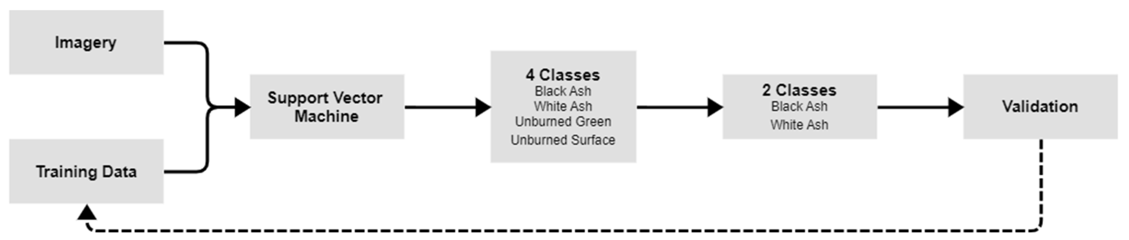
Burn extent classification was performed by using the Support Vector Machine within ArcGIS Pro. Four separate classifications were created for finding the burn extent and severity, one for each of the input rasters. Each classification used the same burn extent training data shapefile as input and was used to train four SVM classifiers, one for each form of input raster. When examining burn extent, these classifications need to be reclassified from four classes to two classes before validation, as burn extent involves the mapping of all pixels as to whether they were burned or not, which can be seen clearly in Figure 2. Four classes were used for classification with the SVM because they were more linearly separable than using two classes, but are not needed in the final classification of burn extent, only in the final classification of biomass consumption [9]. To perform this reclassification step, the Reclassify tool was used within ArcGIS Pro. Validation data was also created for burn extent classification and used to calculate the accuracy of each classification. The methods for creating validation data will be explained in more detail within the next section.
Similarly, biomass consumption can be mapped by using the same four SVM classifiers created from the burn extent classification process. Unlike the burn extent classification process shown in Figure 2 that reclassifies the four classes to two classes (burned and unburned), the biomass consumption process simply validates only the black ash and white ash classes, as everything else is noise and does not contribute to the biomass consumption map.
Figure 3.
Burn Severity (Biomass Consumption) Workflow.
2.5. Validation Data
Validation data is required to find the accuracy of the classification model. In the case of the burn extent classifications, team members digitized polygons over areas of the map where they were confident that the area was either burned or unburned. Similarly, for validating biomass consumption, polygons were digitized in regions that were clearly black ash and white ash. These polygons were created using ArcGIS Pro and saved as a shapefile to be used in further analysis.
Due to the 1.8m spatial resolution of the Worldview2 imagery, the satellite imagery was insufficient in showing the true ground state, making it difficult to observe precise details such as trees. Since drone imagery was acquired within the same location, the drone imagery could be used as a reference when the information within the Worldview2 image was unclear. Using drone imagery to inform how the polygons are drawn on the Worldview2 imagery allowed for more accurate identification of burned and unburned areas. Ideally, validation data could be drawn strictly based on drone imagery, but for the Mesa fire the two images did not quite line up correctly. Even after trying to reproject or transform the coordinate system, the two images were misaligned by only a few meters. Even with the slight misalignment between the Worldview2 and drone imagery, having the hyperspatial drone imagery available to inform selection and labeling of validation data from the Worldview2 images enabled the team to comply with the International Post Burn Validation Protocol which specifies that imagery with higher resolution than that of the mapping layers being developed should be utilized for validation [29].
2.6. Analysis
To calculate the accuracy of each classification, the following steps were taken, both with mapping burn extent and finding biomass consumption. The validation data polygons created were saved as a shapefile and used as input in the Tabulate Area tool in ArcGIS. This tool is used to cross-tabulate areas between two datasets and create a table containing an areal comparison of the classification output rasters against the validation polygons [30]. This tabulate area tool was run 4 times, once for each of the classifications created by the 4 different input rasters. Since the tabulate area tool calculated the area for each combination of classification and validation values of the four classes, these classes were summarized into smaller subgroups for both burn extent and biomass consumption classification. For mapping burn extent, this tool calculates the area in two categories: burned and unburned. Similarly, biomass consumption classification used the tabulate area tool to calculate the area of the black ash and white ash classes. Once the cross-tabulated areas had been calculated, 8 confusion matrices were created.
Using the confusion matrices, shown in Figure 4, which contain the number of pixels that are True Positives (TP), False Positives (FP), True Negatives (TN), and False Negatives (FN), the metrics of accuracy, specificity, and sensitivity could be calculated based on Equations (1) - (3).
3. Results
3.1. Selection
By feeding the burn extent training dataset into the ID3 program, a decision tree was created that can be seen in Figure 5. The bands (attributes) are represented by rectangles, the possible values of each band placed on the edges, and the resulting label placed within circles. Based on the burn extent training dataset, the Yellow band had the most information gain and was included in the exported raster. Since the SVM has no limit on the number of bands allowed, all other bands which contained information crucial to the classification process were also included in the selection: Near Infrared 2, Blue, and Green. These bands were then extracted from Worldview2 imagery, and the resulting raster can be seen in Figure 6.
3.2. Classification
Burn Extent Classification using the SVM resulted in accuracies in between 91 and 96%, with slight variation depending on the raster layer used as input. The RGB bands had the lowest accuracy at 91%, whereas the bands created using Principal Component Analysis and the ID3 had higher accuracies around 95%. Additionally, the specificity of the classification improved from 86% to 92% when either all eight spectral bands were used or some combination based on PCA or the ID3, as opposed to simply using the RGB bands. The full results of the classifications can be seen in Table 1, which show the accuracy, specificity, and sensitivity of each classification based on the four different input layers.
Since specificity involves the calculation of true negatives in relation to the number of all pixels that should have been labeled negative, the specificity is consistently lower than the overall accuracy for each of the classifications. Due to the nature of shadows being incorrectly classified as burned pixels, the number of false positives is raised, decreasing both the accuracy and specificity. Yet, when introducing additional spectral bands besides RGB, the specificity improved by 6 percentage points, showing a possible correlation between using bands outside of the visible spectrum to determine a difference between burned areas and shadows. This issue will be addressed in more detail in the Future Work section of the discussion.
Using the SVM to classify/find biomass consumption resulted in extremely high accuracies, specificities, and sensitivities, with respective averages of 99%, 99.9%, and 98%. As show in Table 2, there was not much noticeable separation between the classifications based on the input raster layer, and these classifications can be seen in further detail within Appendix A.
4. Discussion
The methodology outlined in this paper described the processes for burn extent and severity classifications using Worldview2 imagery as input for a Support Vector Machine. The overall findings were a general success, with burn extent classifications achieving an accuracy exceeding 95% using three PCA bands as inputs (followed closely by all 8 bands and the 3 ID3 bands). Burn severity as measured by biomass consumption classifications averaged greater than 99% regardless of the set of input rasters.
Impact of Shadows on Classification
The Mesa Fire was at a latitude of 44 degrees north. At this and higher latitudes, shadows caused by trees in forested ecosystems will always be present no matter how close to solar noon imagery is taken. The slightly longer than 24-hour temporal resolution of WorldView2 imagery also means that imagery will be taken during different hours of the day, even at times earlier or later in the day when the sun is at a lower angle to the earth, resulting in increased areal extent of shadows resulting from trees and as well as topography. These shadows have proven to be detrimental to the accuracy of the burn extent classifier, due to their misclassification as burned area. This is why the specificity (classified unburned pixels/total unburned pixels) of burn extent is significantly lower than the sensitivity (classified burned pixels/all burned pixels). Future work could be done to mitigate the adverse effects of shadows from imagery, thus increasing specificity and overall accuracy of burn extent classification by reducing false positives when the SVM classifies shadows as burned areas.
Decision Tree Optimization
Another aspect of the project that could be investigated further is increasing efficiency when creating decision trees while analyzing band entropy. The current iteration of the program requires that unique values in each band must first be sorted, then split between each unique value for the band, identifying the optimal spit-point for each attribute in order to identify which of the continuous value bands has the highest information gain. As the dataset increases, both due to increased mapping extent as well as increased radiometric resolution resulting from the use of 16 bit sensors, much more memory and time are required to find the appropriate split points. Additionally, if outliers are present or if the dataset is skewed in any way, the likelihood of the split points providing high levels of information again decreases. To address this issue, the decision tree used within the methodology described above could be optimized to instead use fuzzy logic to determine split points. Machine learning algorithms such as the FID Fuzzy Decision Tree [31] already exist, enabling the user to partition continuous attributes in a more efficient manner. Numerosity reduction [9], [13] could also be evaluated as a means of increasing classification efficiency.
The Precision of Drone and Satellite Imagery
The International Remote Sensing Burn Protocol [29] specifies that validation imagery that is higher resolution than the classification should be utilized when validating mapping products. As mentioned in the methodology section when describing the validation process, it would be preferable to create validation data based on drone imagery. Unfortunately, this is not possible for every fire if no drone imagery has been acquired, but for scenes where both hyperspatial drone imagery and satellite imagery exist, using drone imagery to create the polygons that will be applied to the satellite imagery would allow the user to have a greater degree of confidence throughout more of the image. The use of drone imagery to create validation data is only possible if the drone imagery and satellite imagery are properly spatially registered, with objects in both images having the same coordinates in both images. It was discovered that when the hyperspatial drone imagery and WorldView 2 imagery were both loaded into ArcGIS, objects in the two images were not adequately georegistered, even after attempting to perform a variety of transformations and projections. It was observed that objects in both images could have a spatial displacement of as much as 10 meters between the two images, with an example of this shown in Figure 7. The drone imagery was still very helpful as it allowed users to refer to the higher resolution drone imagery to confirm what they were seeing in the lower resolution WorldView2 imagery. However, validation data could not be digitized directly from the hyperspatial drone imagery without running the risk of the validation polygons not lining up with the classification derived from the WorldView2 image using the SVM.
Removing the Subjectivity Involved in Calculating Accuracy
The current method for finding classifier accuracy in ArcGIS has a problem with its subjectivity. Validation data is manually created, and it needs to encompass every type of problem the classifier could encounter, such as shadows being misclassified as burned areas. The validation data doesn’t need to cover every shadow in the imagery but needs to cover a proportionate area of shadow to the area of total shadow in the imagery in comparison to the rest of the validation data. For example, if a disproportionately high amount of shadows were included in the validation data, the classifier’s accuracy would be incorrectly low because it would be catching too many errors in proportion to the amount of correctly classified areas. If a disproportionately low amount of shadows were included within the validation data, the classifier’s accuracy would be incorrectly high because it wouldn’t be catching enough errors in proportion to the amount of correctly classified area. Due to this problem, accuracy is fully dependent on a person’s ability to perfectly choose validation data that proportionately represents every type of error and success, which isn’t realistic.
Future Work
Additional efforts could attempt to improve calculation of the accuracy metric by reducing this subjective aspect of digitizing and labeling validation data. One possible solution to this issue involves using the Create Accuracy Assessment Points tool within ArcGIS. This tool allows the user to enter a number of points that will be randomly sampled from the raster using stratified random sampling. The user would then be required to label each of the pixels with the appropriate class label. The potential problem with this solution is that the user will not always be confident about what class the random pixel belongs to. When labeling pixels, it is imperative that the person labeling the validation data be certain they are assigning the correct class to each pixel. To account for the possibility of pixels where the class is unclear, the user will need to be able to omit sample pixels, either by removing them from the set of validation pixels or assigning a class of “unknown” that will pull the pixel into a portion of the confusion matrix which can be omitted from the accuracy metric.
There are commercial satellite systems which have very high spatial resolution imagery which could be utilized for acquiring imagery that could be used as a resource for improving the labeling of validation data as well as for inputs for the classifiers. This team investigated the use of Planet SkySat imagery, which has 50cm spatial resolution as well as four bands in the visible as well as near infrared spectra. While SkySat holds immense promise, both as validation as well as classification data source, we also realized that due to the fact that this platform is a tasked resource, the satellite will only acquire imagery if the control team on the ground issues instructions to the satellite to pass over a fire and acquire imagery while it is passing over. Platforms that maintain a consistent orbit, acquiring imagery during regular flyovers, possibly increasing temporal resolution through the use of a multi-platform constellation, will provide a more consistent source of imagery, especially when burn assessment teams initiate the procurement process while developing burn recovery plans after the fire has been contained. Additionally, the availability of post burn imagery from immediately after an area has burned is a critical capability. Extent of high biomass consumption as evidenced by existence of white ash is extremely temporally sensitive due to the susceptibility of white ash to meteorological conditions such as wind and rain [15], making the acquisition of imagery immediately after an area has burned of utmost importance, even if the imagery is stored in an archive from which burn recovery managers can order imagery once they understand what imagery extent will be necessary for mapping a fire once acquiring imagery for a post-burn recovery plan has commenced.
Author Contributions
Conceptualization, D.H. and C.M.; methodology, D.H. and C.M.; software, C.M.; validation, C.M.; formal analysis, C.M. and D.H.; investigation, D.H. and C.M.; resources, D.H.; data curation, D.H. and C.M.; writing—original draft preparation, C.M.; writing—review and editing, C.M. and D.H.; visualization, C.M.; supervision, D.H.; project administration, D.H.; funding acquisition, D.H. All authors have read and agreed to the published version of the manuscript.”.
Funding
This research was funded by Idaho NASA EPSCoR under award 80NSSC19M0043.
Institutional Review Board Statement
Not applicable.
Informed Consent Statement
Not applicable.
Data Availability Statement
All data and source code from this project is available at https://firemap.nnu.edu/worldview-2-materials.
Acknowledgments
We would like to acknowledge the students in the Northwest Nazarene University of Math and Computer Science who have helped with different aspects of this effort, including current and former students Cody Robbins, Bryn Gautier, Carter Katzenberger, Zachary Smith, Parker Bartlow, Cody Lirazan, Kedrick Jones, Daniel Harris, William Gibson, and Daniel Harris. Additionally, we would like to thank Leslie Hamilton for reviewing the submitted manuscript.
Conflicts of Interest
The authors declare no conflict of interest.
Appendix A. Burn Extent Classification Visualization
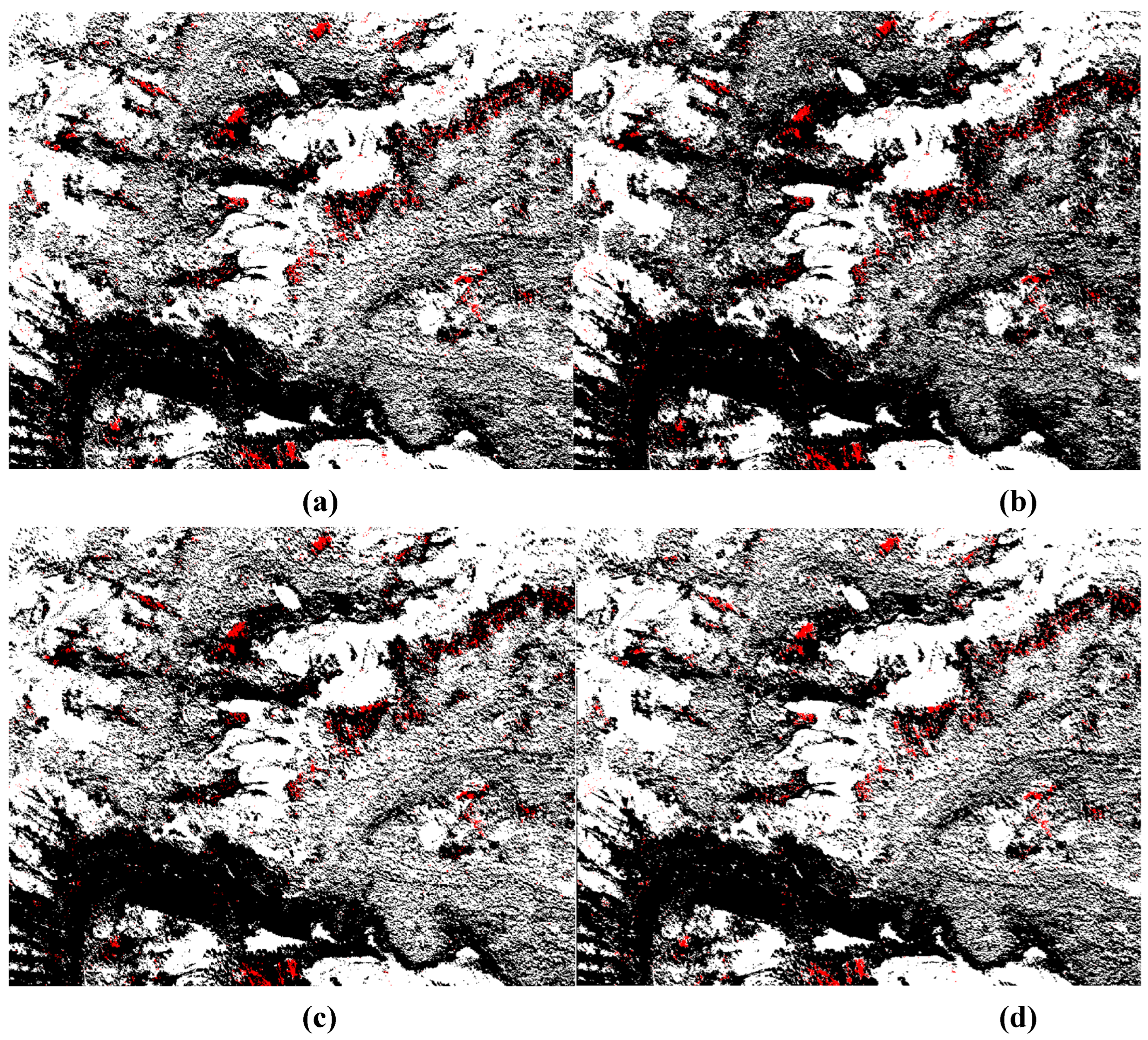
Each of the following figures contains 4 images:
- A.
- Raster input.
- B.
- The initial Burn Extent Classification that resulted in four classes: black ash (black), white ash (grey), unburned greenery (green), and unburned surface (orange).
- C.
- The reclassified Burn Extent Classification represented by only two classes: burned (black) and unburned pixels (grey).
- D.
- The reclassified Biomass Consumption Classification represented by two classes: black ash (black) and white ash (red), with all unburned areas not represented by any color.
Figure A1.
Biomass Consumption and Burn Extent Classifications based on RGB Worldview 2 Imagery (a) RGB Worldview 2 Imagery (b) Initial Burn Extent Classification (c) Reclassified Burn Extent (d) Biomass Consumption.
Figure A1.
Biomass Consumption and Burn Extent Classifications based on RGB Worldview 2 Imagery (a) RGB Worldview 2 Imagery (b) Initial Burn Extent Classification (c) Reclassified Burn Extent (d) Biomass Consumption.
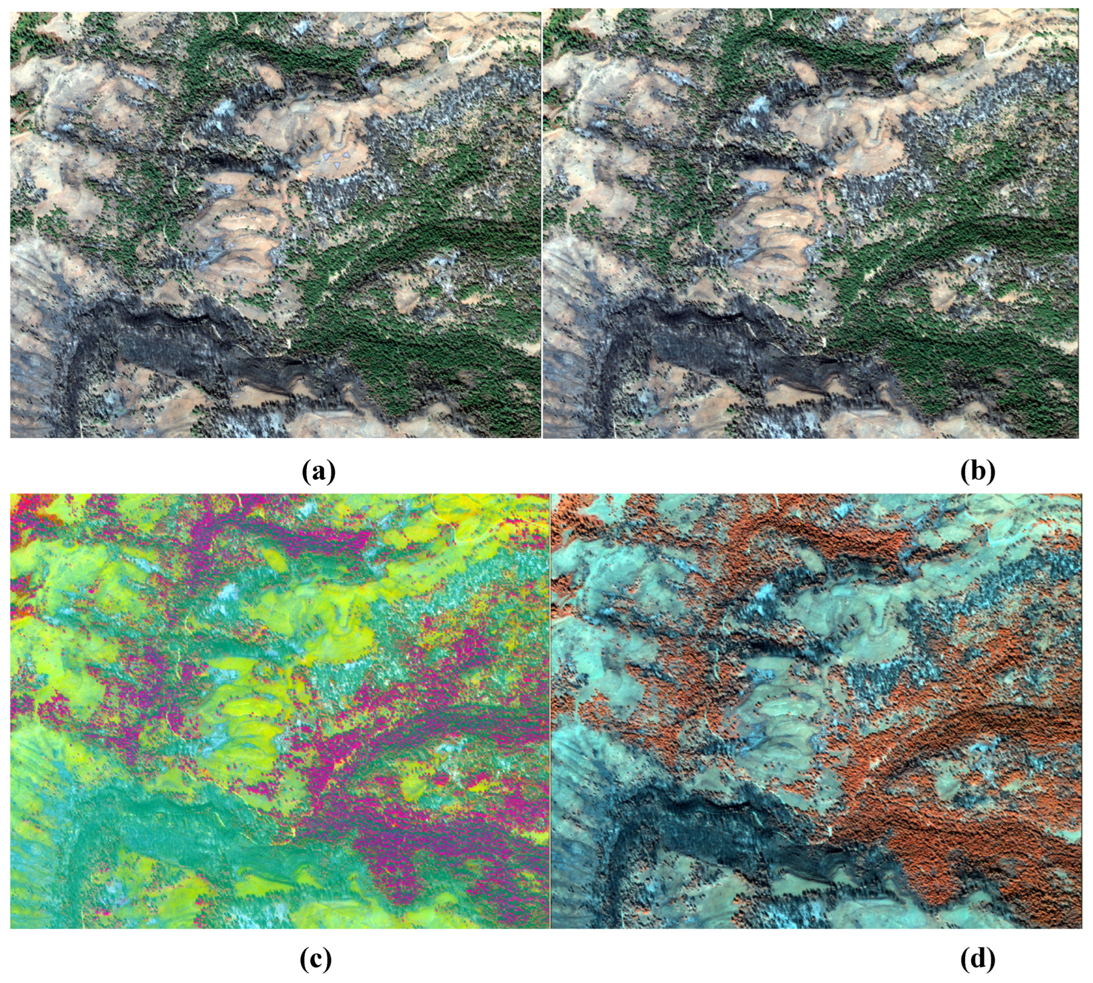
Figure A2.
Biomass Consumption and Burn Extent Classifications based on Original Worldview 2 Imagery with all 8 spectral bands (a) 8 Band Worldview 2 Imagery (b) Initial Burn Extent Classification (c) Reclassified Burn Extent (d) Biomass Consumption.
Figure A2.
Biomass Consumption and Burn Extent Classifications based on Original Worldview 2 Imagery with all 8 spectral bands (a) 8 Band Worldview 2 Imagery (b) Initial Burn Extent Classification (c) Reclassified Burn Extent (d) Biomass Consumption.
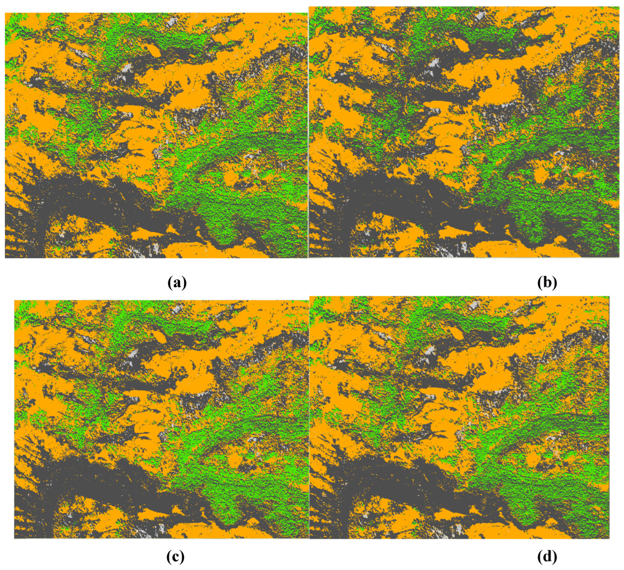
Figure A3.
Biomass Consumption and Burn Extent Classifications based on PCA-Transformed Worldview 2 Imagery with Reduced Dimensionality (a) 8 Band Worldview 2 Imagery (b) Initial Burn Extent Classification (c) Reclassified Burn Extent (d) Biomass Consumption.
Figure A3.
Biomass Consumption and Burn Extent Classifications based on PCA-Transformed Worldview 2 Imagery with Reduced Dimensionality (a) 8 Band Worldview 2 Imagery (b) Initial Burn Extent Classification (c) Reclassified Burn Extent (d) Biomass Consumption.
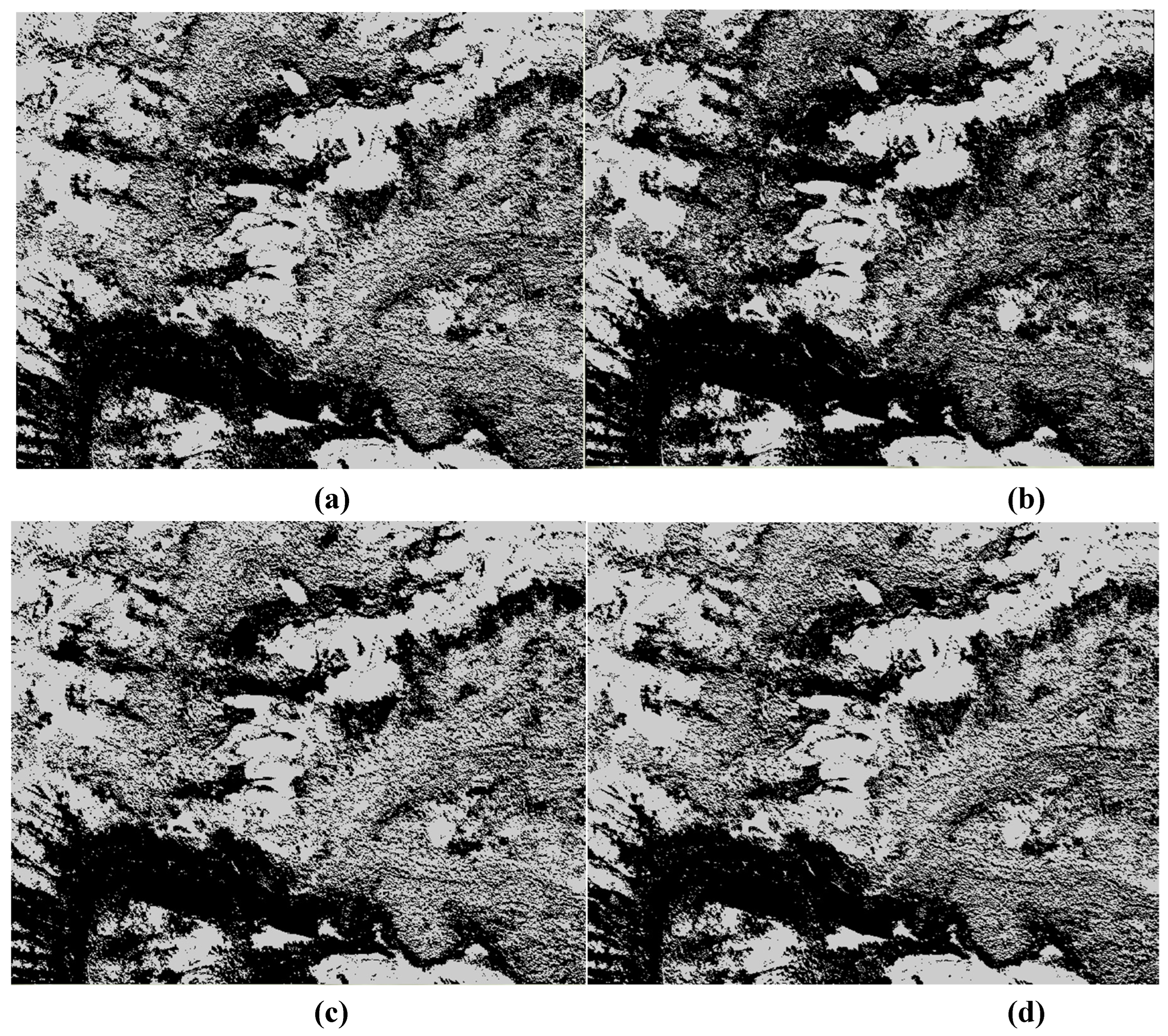
Figure A4.
Biomass Consumption and Burn Extent Classifications based on Worldview 2 Imagery containing Spectral Bands based on ID3 Results (a) 8 Band Worldview 2 Imagery (b) Initial Burn Extent Classification (c) Reclassified Burn Extent (d) Biomass Consumption.
Figure A4.
Biomass Consumption and Burn Extent Classifications based on Worldview 2 Imagery containing Spectral Bands based on ID3 Results (a) 8 Band Worldview 2 Imagery (b) Initial Burn Extent Classification (c) Reclassified Burn Extent (d) Biomass Consumption.
References
- National Aeronautics and Space Administration, “Commercial Smallsat Data Acquisition (CSDA) Program | Earthdata,” 2023. https://www.earthdata.nasa.gov/esds/csda (accessed Mar. 29, 2023).
- Wildland Fire Leadership Council, “The national strategy: the final phase in the development of the National Cohesive Wildland Fire Management Strategy,” Washington, DC) Available at http://www. forestsandrangelands. gov/strategy/documents/strategy/CSPhaseIIINationalStrategyApr2014. pdf [Verified 11 December 2015], 2014.
- K. Hoover and L. A. Hanson, “Wildfire Statistics,” Congressional Research Service, Dec. 2022. Accessed: Feb. 10, 2023. [Online]. Available: https://crsreports.congress.gov/product/pdf/IF/IF10244.
- National Interagency Fire Center, “Suppression Costs,” 2022. https://www.nifc.gov/fire-information/statistics/suppression-costs (accessed Feb. 10, 2023).
- National Wildfire and Coordinating Group, “NWCG Report on Wildland Firefighter Fatalities in the United States: 2007-2016,” Dec. 2017. Accessed: Feb. 10, 2023. [Online]. Available: https://www.nwcg.gov/sites/default/files/publications/pms841.pdf.
- G. Zhou, C. Li, and P. Cheng, “Unmanned aerial vehicle (UAV) real-time video registration for forest fire monitoring,” in Proceedings. 2005 IEEE International Geoscience and Remote Sensing Symposium, 2005. IGARSS ’05., Seoul, South Korea, Jul. 2005. [CrossRef]
- Insurance Information Institute, “Facts + Statistics: Wildfires | III,” Feb. 10, 2023. https://www.iii.org/fact-statistic/facts-statistics-wildfires (accessed Feb. 10, 2023).
- J. C. Eidenshink, B. Schwind, K. Brewer, Z.-L. Zhu, B. Quayle, and S. M. Howard, “A project for monitoring trends in burn severity,” Fire ecology, vol. 3, no. 1, pp. 3–21, 2007. [CrossRef]
- D. Hamilton, “Improving Mapping Accuracy of Wildland Fire Effects from Hyperspatial Imagery Using Machine Learning,” The University of Idaho, 2018.
- National Aeronautics and Space Administration (NASA), “Landsat 9 Instruments,” NASA, Feb. 13, 2023. http://www.nasa.gov/content/landsat-9-instruments (accessed Feb. 13, 2023).
- J. E. Keeley, “Fire intensity, fire severity and burn severity: a brief review and suggested usage,” Int.J.Wildland Fire, vol. 18, no. 1, pp. 116–126, 2009. [CrossRef]
- C. H. Key and N. C. Benson, “Landscape Assessment (LA),” In: Lutes, Duncan C.; Keane, Robert E.; Caratti, John F.; Key, Carl H.; Benson, Nathan C.; Sutherland, Steve; Gangi, Larry J. 2006. FIREMON: Fire effects monitoring and inventory system. Gen. Tech. Rep. RMRS-GTR-164-CD. Fort Collins, CO: U.S. Department of Agriculture, Forest Service, Rocky Mountain Research Station. p. LA-1-55, vol. 164, 2006, Accessed: Apr. 28, 2023. [Online]. Available: https://www.fs.usda.gov/research/treesearch/24066. [CrossRef]
- D. Hamilton, B. Myers, and J. Branham, “Evaluation of Texture as an Input of Spatial Context for Machine Learning Mapping of Wildland Fire Effects,” Signal and Image Processing: An International Journal, vol. 8, no. 5, 2017. [CrossRef]
- L. B. Lentile et al., “Remote sensing techniques to assess active fire characteristics and post-fire effects,” Int. J. Wildland Fire, vol. 15, no. 3, p. 319, 2006. [CrossRef]
- A. T. Hudak, R. D. Ottmar, R. E. Vihnanek, N. W. Brewer, A. M. S. Smith, and P. Morgan, “The relationship of post-fire white ash cover to surface fuel consumption,” Int. J. Wildland Fire, vol. 22, no. 6, pp. 780–786, 2013. [CrossRef]
- J. H. Scott and E. D. Reinhardt, “Assessing crown fire potential by linking models of surface and crown fire behavior,” USDA Forest Service Research Paper, no. Journal Article, p. 1, 2001. [CrossRef]
- D. Hamilton, K. Brothers, C. McCall, B. Gautier, and T. Shea, “Mapping Forest Burn Extent from Hyperspatial Imagery Using Machine Learning,” Remote Sensing, vol. 13, no. 19, Art. no. 19, Jan. 2021. [CrossRef]
- J. Han, M. Kamber, and J. Pei, Data Mining: Concepts and Techniques, Third. Amsterdam: Morgan Kaufmann, 2012.
- D. Hamilton, R. Pacheco, B. Myers, and B. Peltzer, “kNN vs. SVM: a Comparison of Algorithms,” in Proceedings of the Fire Continuum - Preparing for the future of wildland fire. 2018 May 21-24, Missoula, MT: Proceedings RMRS-P-78. Fort Collins, CO: U.S. Department of Agriculture, Forest Service, Rocky Mountain Research Station., 2020, p. 95. [Online]. Available: https://www.fs.usda.gov/treesearch/pubs/60581.
- O. Zammit, X. Descombes, and J. Zerubia, “Burnt area mapping using support vector machines,” For.Ecol.Manage., vol. 234, no. 1, p. S240, 2006. [CrossRef]
- G. P. Petropoulos, W. Knorr, M. Scholze, L. Boschetti, and G. Karantounias, “Combining ASTER multispectral imagery analysis and support vector machines for rapid and cost-effective post-fire assessment: a case study from the Greek wildland fires of 2007,” Natural Hazards and Earth System Sciences, vol. 10, no. 2, pp. 305–317, Feb. 2010. [CrossRef]
- European Space Agency (ESA), “WorldView-2 - Earth Online,” WorldView-2 Instruments, Feb. 13, 2023. https://earth.esa.int/eogateway/missions/worldview-2 (accessed Feb. 13, 2023).
- Satellite Imaging Corporation, “WorldView-2 Satellite Sensor | Satellite Imaging Corp,” Feb. 13, 2023. https://www.satimagingcorp.com/satellite-sensors/worldview-2/ (accessed Feb. 13, 2023).
- S. Russell and P. Norvig, Artificial intelligence : A modern approach, Fourth. in Pearson Series in Artificial Inteligence, no. Book, Whole. Hoboken, NJ: Pearson Education, 2020.
- Environmental Sciences Research Institute, “Image Classification Wizard—ArcGIS Pro | Documentation,” 2023. https://pro.arcgis.com/en/pro-app/latest/help/analysis/image-analyst/the-image-classification-wizard.htm (accessed Mar. 28, 2023).
- D. Hamilton, B. Myers, and J. Branham, “Evaluation of Texture as an Input of Spatial Context for Machine Learning Mapping of Wildland Fire Effects,” Signal and Image Processing: An International Journal, vol. 8, no. 5, 2017. [CrossRef]
- Environmental Sciences Research Institute, “How Principal Components works—ArcGIS Pro | Documentation,” 2023. https://pro.arcgis.com/en/pro-app/latest/tool-reference/spatial-analyst/how-principal-components-works.htm (accessed Apr. 05, 2023).
- Environmental Sciences Research Institute, “Train Support Vector Machine Classifier (Spatial Analyst)—ArcGIS Pro | Documentation,” 2023. https://pro.arcgis.com/en/pro-app/latest/tool-reference/spatial-analyst/train-support-vector-machine-classifier.htm (accessed Mar. 28, 2023).
- L. Boschetti, D. P. Roy, and C. O. Justice, “International Global Burned Area Satellite Product Validation Protocol Part I–production and standardization of validation reference data.” 2009. Accessed: Aug. 17, 2021. [Online]. Available: https://lpvs.gsfc.nasa.gov/PDF/BurnedAreaValidationProtocol.pdf.
- Environmental Sciences Research Institute, “Tabulate Area (Spatial Analyst)—ArcGIS Pro | Documentation,” 2023. https://pro.arcgis.com/en/pro-app/latest/tool-reference/spatial-analyst/tabulate-area.htm (accessed Apr. 05, 2023).
- C. Z. Janikow and K. Kawa, “Fuzzy Decision Tree FID,” in NAFIPS 2005 - 2005 Annual Meeting of the North American Fuzzy Information Processing Society, Detroit, MI, USA: IEEE, 2005, pp. 379–384. [CrossRef]
Figure 1.
(a) Mesa Fire Location over topographical base map layer. (b) Mesa Fire Perimeter from MTBS in Red with the AOI in Black.
Figure 1.
(a) Mesa Fire Location over topographical base map layer. (b) Mesa Fire Perimeter from MTBS in Red with the AOI in Black.
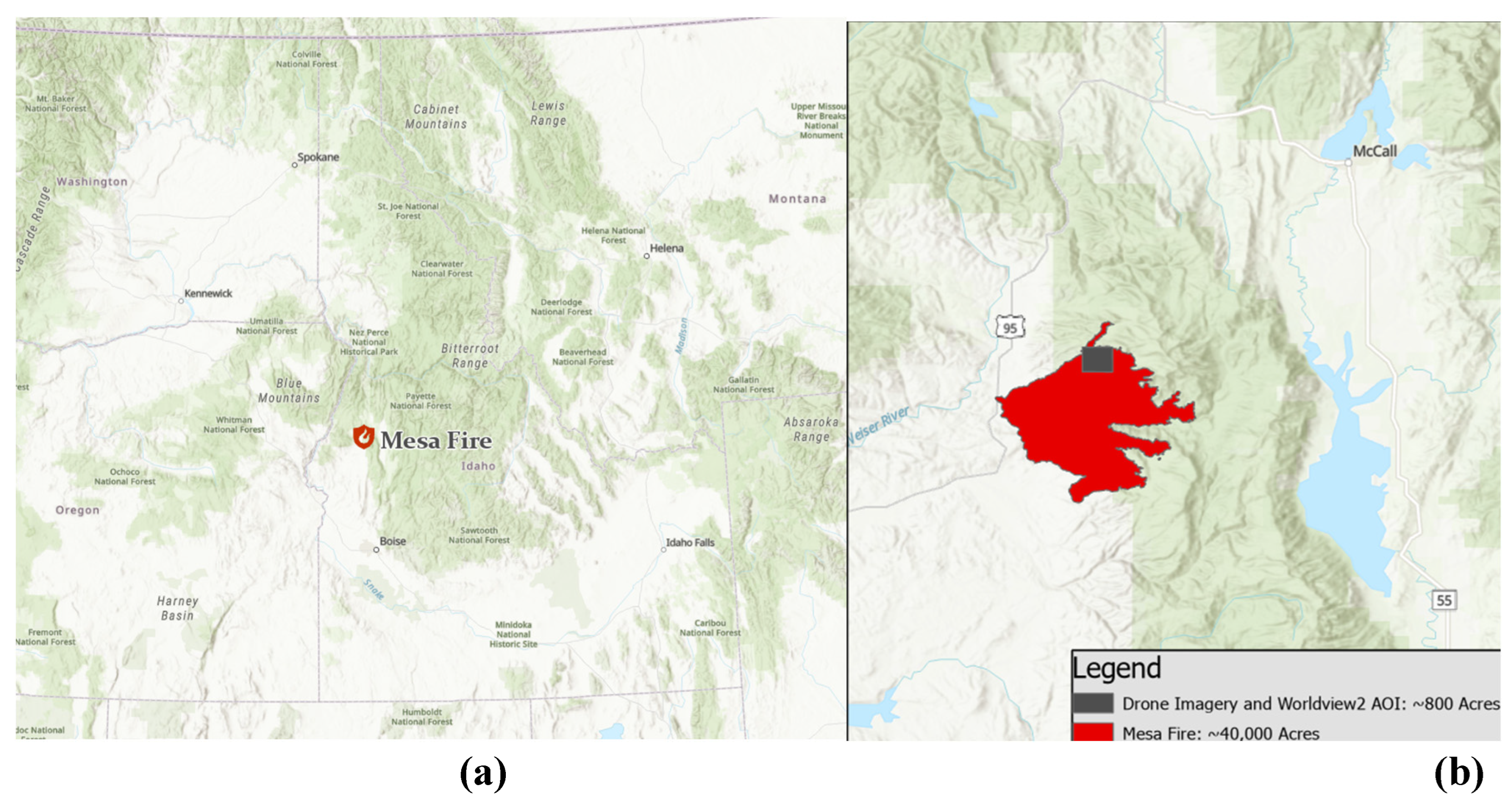
Figure 2.
Burn Extent Classification Workflow.
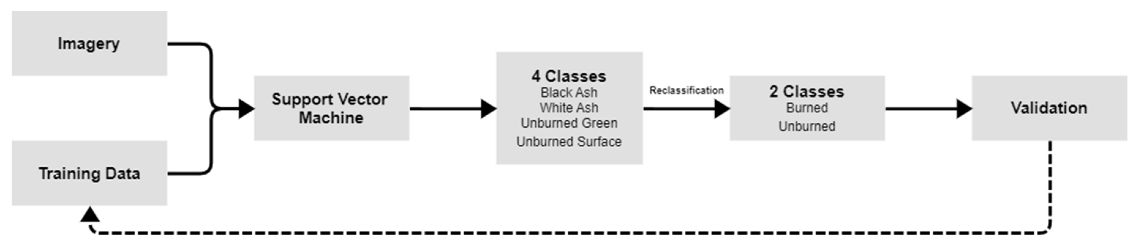
Figure 4.
Components of a Confusion Matrix.
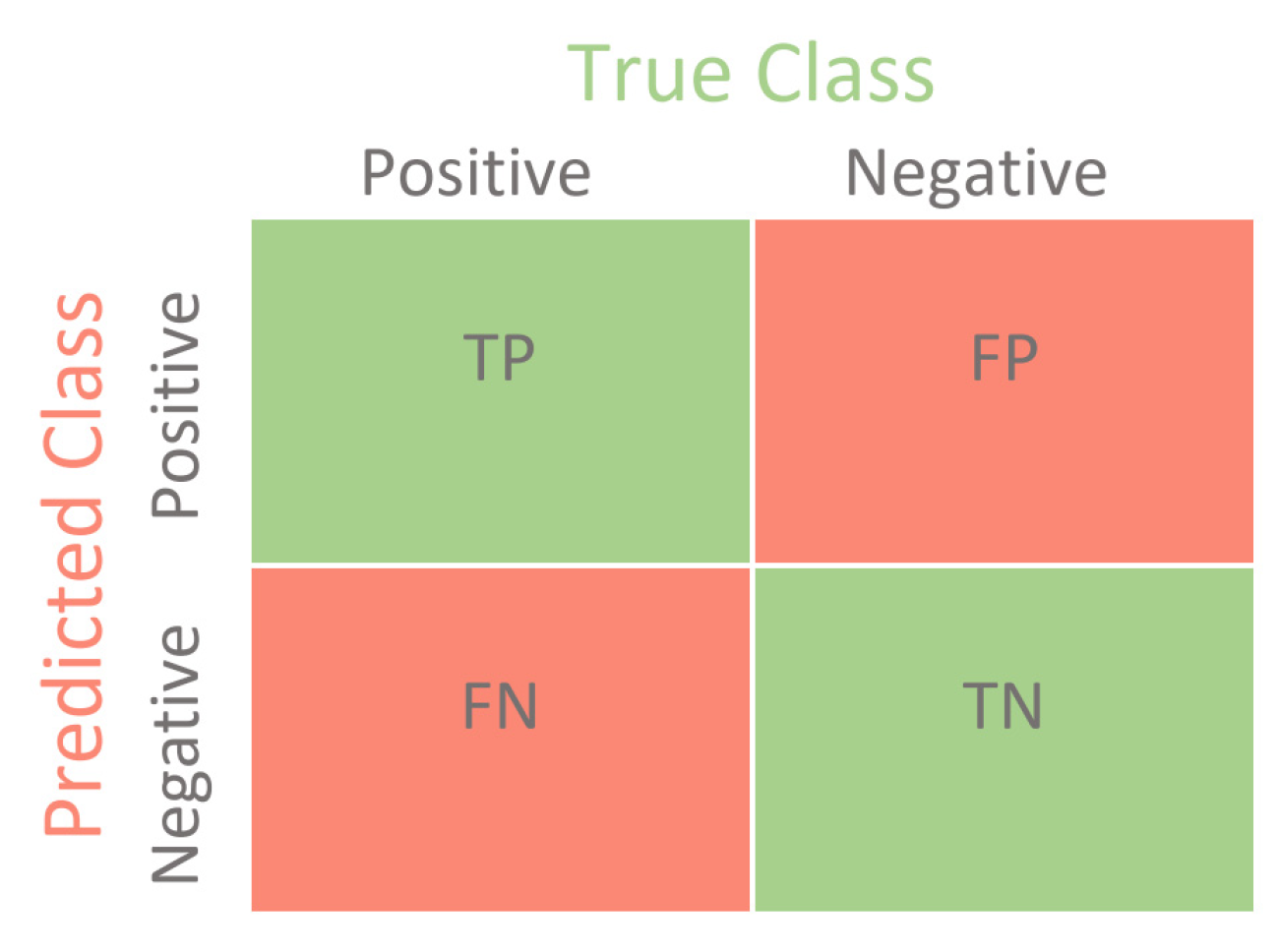
Figure 5.
Burn Extent Decision Tree.
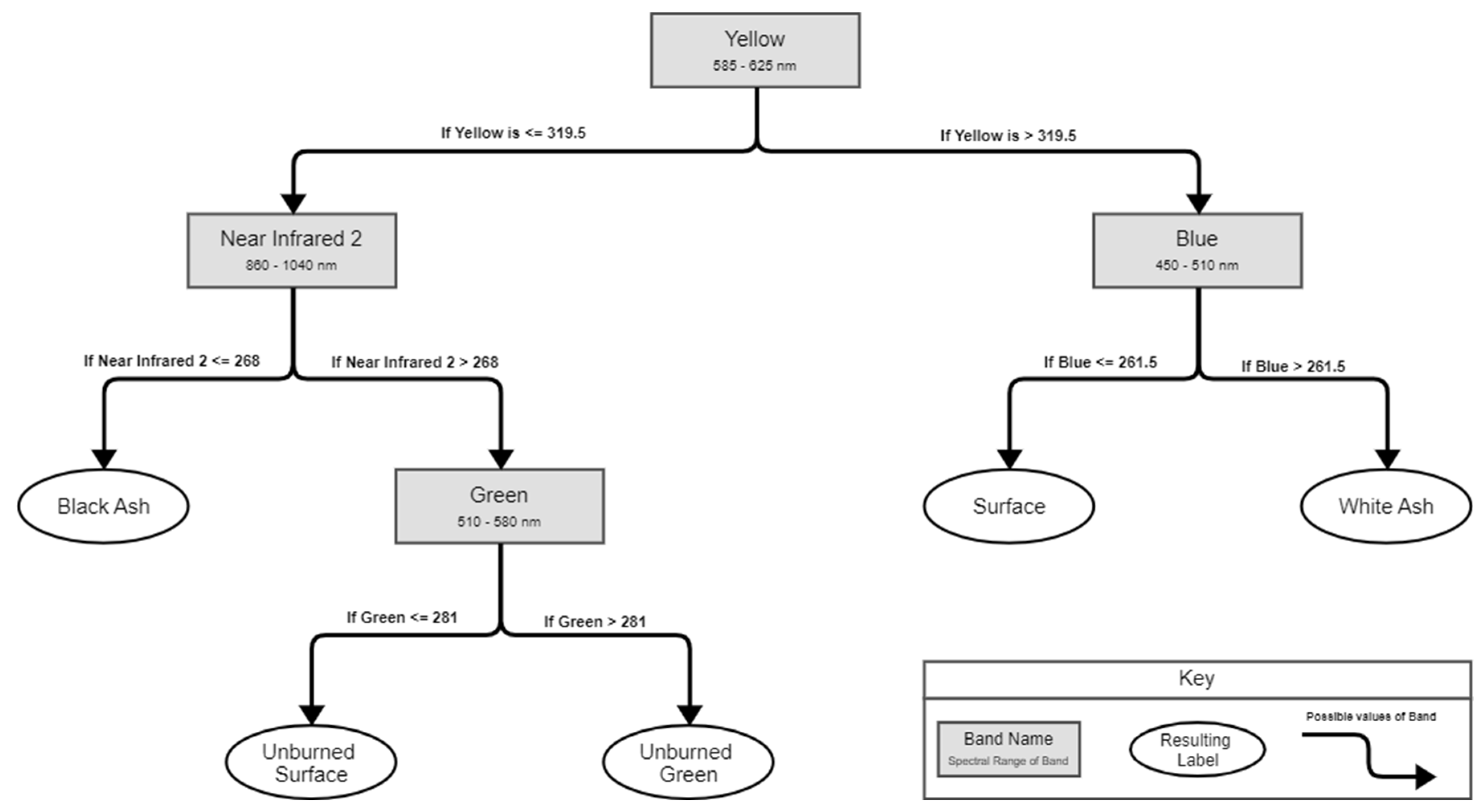
Figure 6.
Extracted Bands based on Burn Extent Decision Tree.
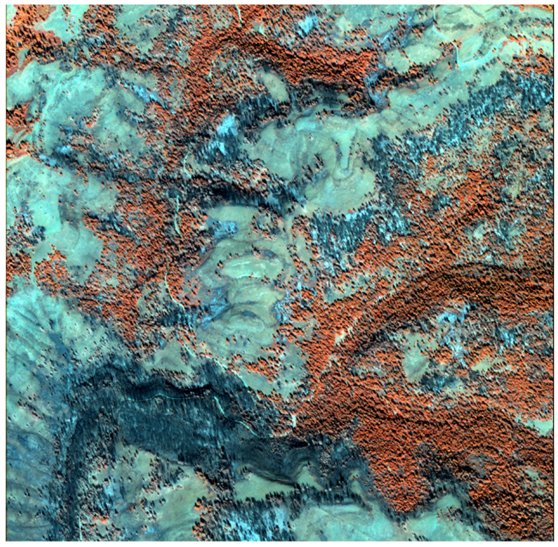
Figure 7.
Representation of Spatial Displacement between Drone and Worldview2 Imagery (a) Overview of the Mesa Fire area where hyperspatial drone imagery was acquired, with the region that will be zoomed in within the red box. (b) Hyperspatial drone imagery within the red polygon, with a digitized road layer in black. (c) Worldview2 imagery within the red polygon, with a digitized road layer in black, slightly off from where the road is in the drone imagery.
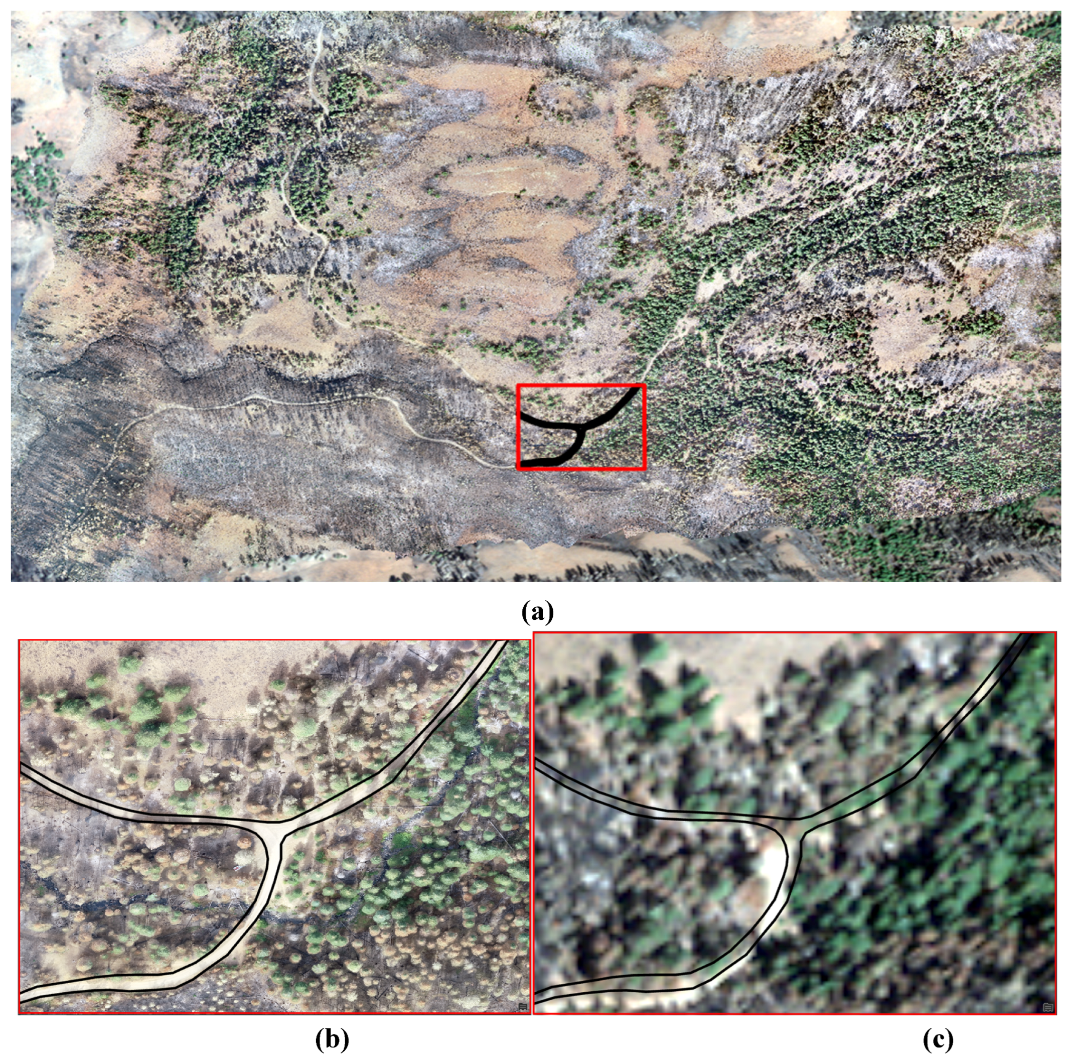

Table 1.
Results from Burn Extent Classification.
| Input Layer | Accuracy | Specificity | Sensitivity |
| Worldview2 RGB Bands | 91.37% | 86.25% | 94.72% |
| All 8 Worldview 2 Bands | 94.44% | 92.23% | 95.89% |
| PCA-Transformed Bands | 95.25% | 92.26% | 97.20% |
| ID3-Selected Bands | 94.97% | 92.15% | 96.81% |
| Average | 94.01% | 90.72% | 96.16% |
Table 2.
Results from Biomass Consumption Classification.
| Input Layer | Accuracy | Specificity | Sensitivity |
| Worldview2 RGB Bands | 99.54% | 99.95% | 98.94% |
| All 8 Worldview 2 Bands | 99.29% | 99.95% | 98.35% |
| PCA-Transformed Bands | 98.48% | 100.00% | 96.33% |
| ID3-Selected Bands | 99.66% | 99.95% | 99.26% |
| Average | 99.14% | 99.97% | 97.98% |
Disclaimer/Publisher’s Note: The statements, opinions and data contained in all publications are solely those of the individual author(s) and contributor(s) and not of MDPI and/or the editor(s). MDPI and/or the editor(s) disclaim responsibility for any injury to people or property resulting from any ideas, methods, instructions or products referred to in the content. |
© 2023 by the authors. Licensee MDPI, Basel, Switzerland. This article is an open access article distributed under the terms and conditions of the Creative Commons Attribution (CC BY) license (http://creativecommons.org/licenses/by/4.0/).
Copyright: This open access article is published under a Creative Commons CC BY 4.0 license, which permit the free download, distribution, and reuse, provided that the author and preprint are cited in any reuse.


