3.1. Lognormal modeling
For this work, we used an approach similar to [
11] but adopting a sum of time-shifted and scaled lognormal density functions rather than scaled normal density functions. We favor lognormal over normal functions for such modeling for multiple reasons. First, lognormal transfert functions are causal. They have a support that starts at a specific time
(see (
1)), as opposed to an
support for the normal equation. Further, the use of sums of lognormal functions for modeling biological time-series has been well-developed for the study of motor control [
13,
14,
15,
16]. The biological relevance of the lognormal as a transfer function is well-rooted mathematically through the Central Limit Theorem, as applied to biological networks of subprocesses coupled through proportionality. This contrasts with the response of a system made of independent and additive subprocesses, which converges, under the same theorem, toward a normal response. These ideas have been developed in detail in the context of the Lognormality Principle [
17,
18].
In terms of interpreting the meaning of lognormal parameters, (in seconds) represents the time when the lognormal process was initiated. Since lognormal-shaped waveforms are emerging from the convergence of small effects associated with many coupled subsystems, we can see as the moment the first cells generated an action potential and triggered an avalanche of subsequent action potentials in the network of neighboring cells. The parameter D represents the amplitude of the equivalent electrical dipole created by this process. More precisely, it is equal to the integration over time of the depolarization or repolarization waves (in ). The parameters and represent, on a logarithmic scale, the time delay and response time of the network of excitable cells. Therefore, these parameters are emergent properties due to the speed of propagation of the electrical waves in these networks. We expect their values to reflect biological properties that modulate the propagation speed, such as the strength of gap-junction coupling between neighboring cells.
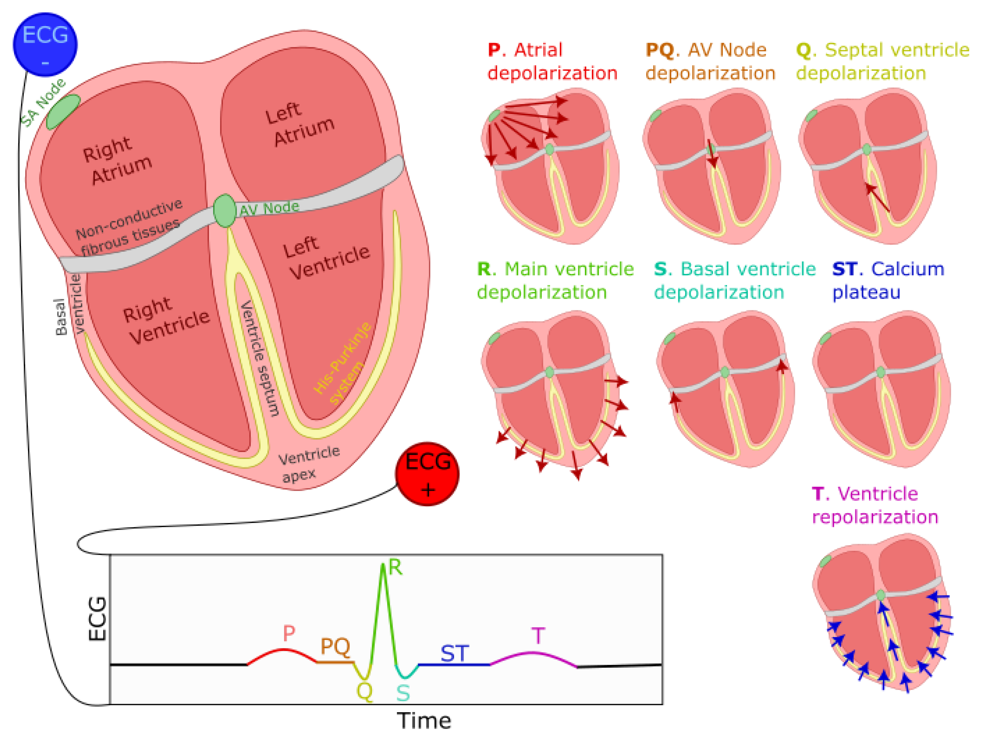
In this approach, a PQRST complex is constituted of six partly overlapping lognormal equations (
1). The P, Q, R, and S waves are all represented by a single equation. For expediency, we accounted for the negative skew of the T wave by representing it with the subtraction of two lognormals (noted
and
). Further investigation will be required to understand the physiological underpinning of this negative skew and, consequently, the most biologically-relevant way to model it.
3.4. The PQRST lognormal prototype
The inverse modeling (i.e., curve fitting) constitutes a significant difficulty when modeling time-series with sums of lognormal functions. Various algorithms have been developed to extract parameters for such models [
20,
21,
22,
23]. These extractors perform reasonably well, but the difficulty of this regression problem leaves a place for improvement. For our application, we want to benefit from the ability to map lognormal components between time-series provided by the prototype-based extraction [
21]. We can adopt this approach where modeling time-series with a stereotypical shape, as is the case for the PQRST complex. With that method, we embed our
prior knowledge of the problem and our hypotheses about the generation of the observed signals by defining a starting solution (i.e., a
prototype) made by a series of lognormal components. Then, we obtain the final solutions by adjusting this prototype to every sample, fitting the lognormal parameters to account for individual differences.
However, one issue with the least-square regression of prototypes is that such optimal solutions, if not properly constrained, can drift away from the conceptual modeling of the generative process captured by the prototype. For example, in this case, a lognormal component initially set in the prototype to model the P components can drift and end up modeling slight noise-related deviations in high-amplitude components such as the R component. Although this is not a problem for obtaining a good curve fitting, it becomes an issue when studying the distributions of the parameters, e.g., associated with the P component. That is, although potentially providing an optimal curve fitting, such optimization may not hit the right balance between fitting the observation and providing a plausible solution in terms of the biological or physiological mechanisms of the process being modeled.
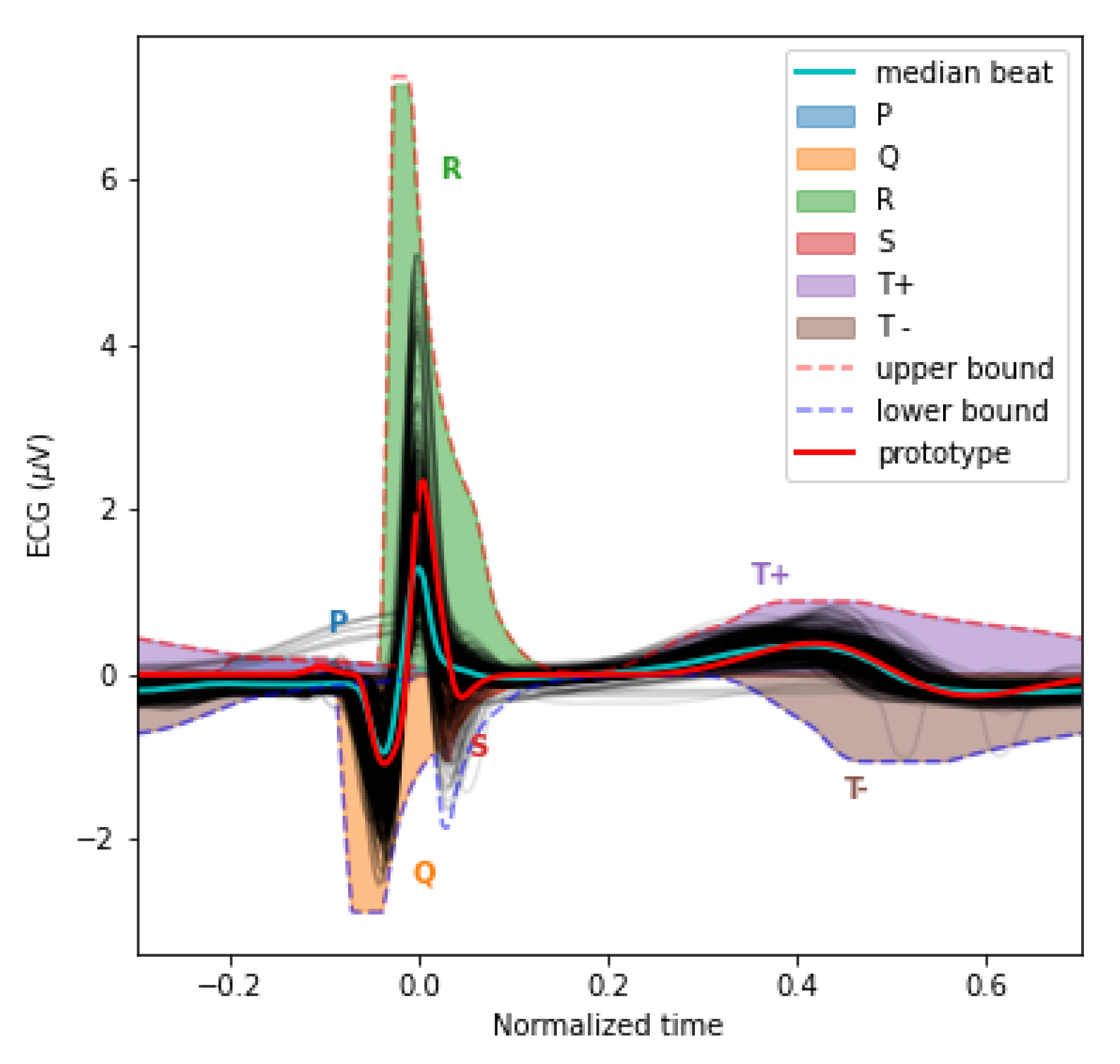
To help constrain our prototype, we used upper and lower bounds for the PQRST complexes. These bounds are defined analytically from box constraints on the lognormal parameters (
4-
7) (see [
20] for the derivation of these bounds). The
Figure 3 illustrates the envelope of all PQRST complexes generated by this
sigma-lognormal (i.e., sum of lognormals) model, given the bounds we selected (see
Table 1). We chose these bounds as a trade-off between encompassing the mean PQRST complexes of all recordings (except some apparent outliers) while constraining the possible solutions to minimize the proportion of the parameter space that can produce PQRST time-series that are not physiologically plausible. These bounds were derived from the parameters
of the prototype
such that
, except for 1) the value of the
parameters being ceiled or floored to 0 when their interval intersects 0, and 2) for
. The first exception ensures that the qualitative interpretation of the different waves remains intact. A sign inversion for a
D parameter would mean changing a depolarization wave into a repolarization wave, or vice-versa. Such a conversion is not possible in normal physiological conditions. For example, the P wave can only be due to the depolarization of the myocardial cells of the atrium. We will never observe a hyperpolarizing wave, rather than depolarizing wave, being caused by an inversion of this process. Alternatively, such polarity reversal could be due to technical issues, such as a misplacement of the electrodes. However, these acquisition problems should be managed when preprocessing the recordings rather than being captured by the model parameters. We used the second exception for a pragmatic reason; we needed to allow the
parameter to vary within a wider range to include most of the recorded PQRST complexes within the established bounds. With respect to the
term, the
notation denotes the absolute value of
, and the indices in
,
, and
stand for "prototype", "upper bound", and "T wave of the prototype", respectively. Other indices are derived using the same logic. The prototype was obtained by manually fitting a sigma-lognormal curve that captures the general trend of our sample of beat profiles. Its parameters are given in
Table 2.
3.5. Reinforcement learning for parameter extraction
For this project, we used the Stable-Baselines3 and OpenAI Gym Python packages to implement a deep reinforcement learning approach for fitting our lognormal model to PQRST time-series. We aim to improve over the grid optimization algorithm previously used to adjust the sigma-lognormal prototype to recorded time-series. We adopted reinforcement learning for this problem because it can find optimal solutions to problems for which the "true" or "best" solution is not known in advance, as long as we can define a measure of the quality of a solution. In our case, the root-mean-square fitting error can serve as such a measure. As opposed to classical supervised learning, reinforcement learning is not limited by the quality of the training data (i.e., it can adapt and become better than experts at a given task). Further, the reinforcement learning approach is interesting because the active development of Bayesian reinforcement learning [
24]. We expect future Bayesian extensions to provide a more appropriate way to integrate prior knowledge into the estimation process by using prior distributions in the definition of the prototype instead of point values and box constraints (see the Discussion section).
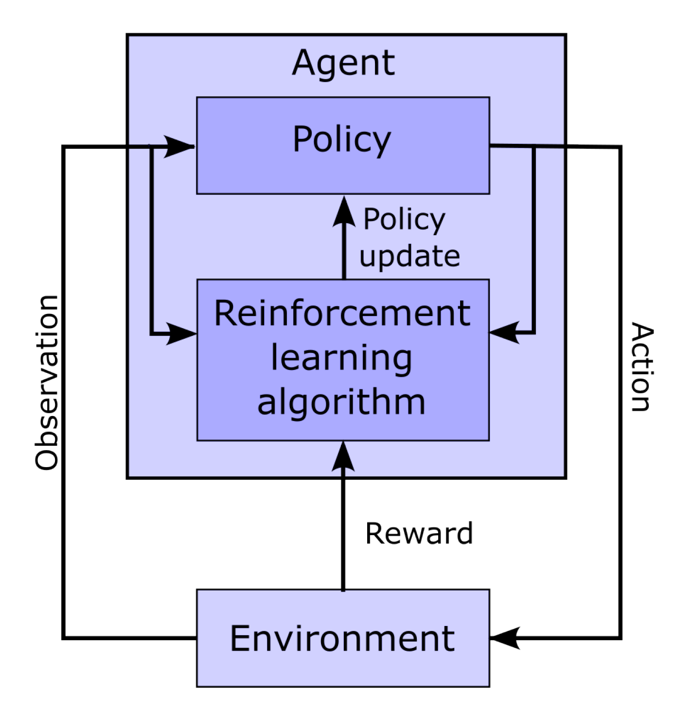
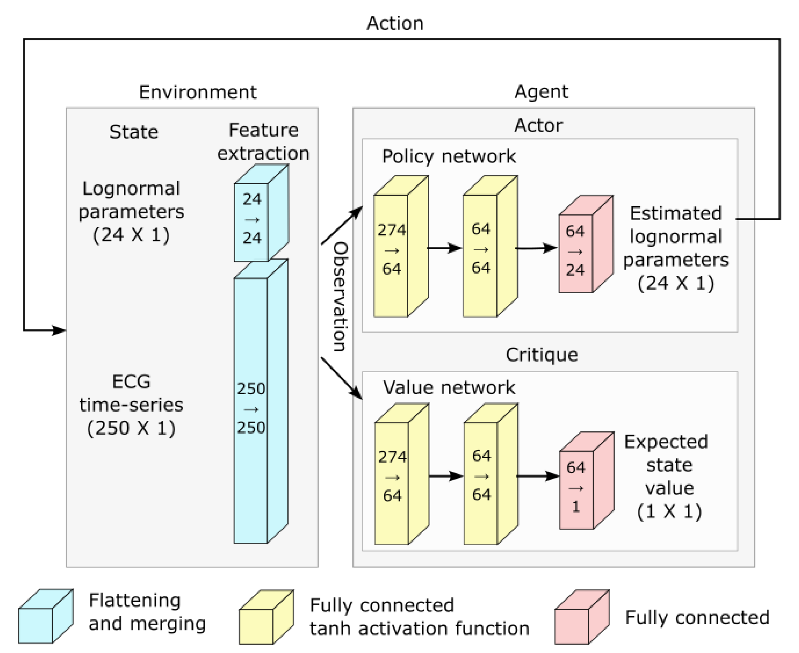
Figure 4 shows a classic schematic representation of reinforcement learning, illustrating the interplay between the learning agent and its environment. In that paradigm, the policy maps the current state of the environment to the probability of performing given actions. This policy captures the transition probability of a Markovian decision process, as it does not depend on past states. In this context, the learning task boils down to optimizing the policy so that actions leading to the highest rewards have the highest probability of being executed. To implement such an approach, the space of possible actions, the observations space (i.e., the observable environment states), and the reward must first be defined.
Action space: Our model has 24 parameters. We consider these as latent variables. The parameter space is defined as a bounded box in
, and the upper bound
and the lower bound
have already been defined in the previous section. We define a reference point as the middle of this bounded box, i.e.,
. At the start of the fitting process, the estimated solution is set equal to
, where the index in
indicates the step number, with 0 standing for the initial estimate. The action space is a box
. At each step of the fitting process, the action
taken by the agent is used to update the estimated solution following the rule
. However, we note that even within this relatively narrow box, the sigma-lognormal parameters can take values such that the order of the PQRST lognormal components gets changed (i.e., the Q component may move after the R component). Since such an inversion is contrary to the intent of the model, we further constrain this ordering. To this end, we first define the order of lognormal components by the timing of their peak. For a lognormal defined by parameters
(as defined in (
2)), this peak can be shown to happen at time
. Thus, we constrain the impact of the action on
so that it is canceled whenever it would results in
(i.e., the action is such that it would cause the timing of the peaks of two consecutive components to get inverted), with
j and
referring to two consecutive lognormal components in the set of
components. We further limit the action so that the resulting parameters remain within the box defined by
and
.
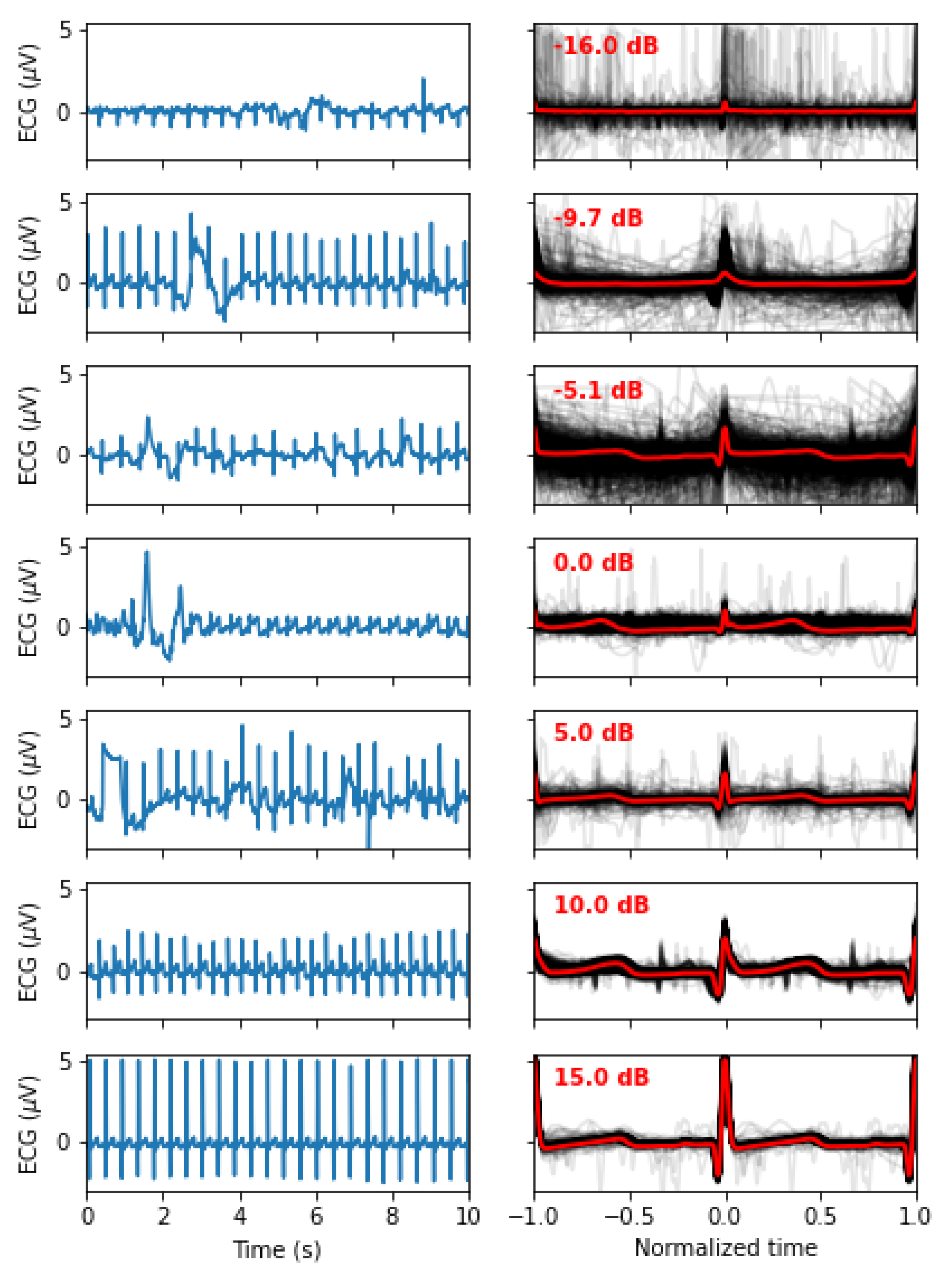
Observation space: The observation space for this model is a dictionary containing values for the estimated parameters and the fitting errors. The space for the fitting errors is a box of dimension 250. The PQRST signals are normalized to 500 points equally spaced between -1 and +1 (see the Preprocessing section), but we observe only half of this interval, between -0.3 and 0.7. ECG signals in the remaining portion of the normalized time interval are mostly flat and contain little information. We set lower and upper bounds for that box at 1.5 times the minimum and maximum values observed for each of these points across all recorded PQRST time-series. Observed values for the fitting error are taken as the difference between the PQRST time-series being analyzed and the signal synthesized from . The observation space for the estimated parameters is the 24-dimensional box bounded by and , and the observed values are . We further normalized the observation space, as is generally recommended when using a heterogeneous observation space. We confirmed that the normalization of the observation space resulted in a significant improvement in performance for our application.
Reward: In reinforcement learning, the reward is the objective function to maximize, and it depends on the action performed. Thus, reinforcement learning algorithms aim at finding the action that maximizes the reward associated with any given state. For our application, the reward is defined as the difference in fitting SNR before and after the action was taken.
Training: The optimization of a PQRST time-series terminates when the algorithm reaches its maximal number of steps (1000) or when the agent fails to find a solution (i.e., a set of parameter values) improving over its best SNR for 100 consecutive steps. Every time the optimization of a PQRST time-series terminated, another time-series was picked at random, and a new optimization was started. We trained our model for a total of 3,000,000 steps, at which point performances were stable, and no additional training seemed likely to provide any advantage.
For learning, we implemented a deep reinforcement learning solution based on the Proximal Policy Optimization (PPO) [
25] scheme. This relatively new algorithm has been designed to control the size of the steps taken when doing the gradient-based optimization of the policy. Large steps in the optimization process can result in instability as they can push the optimizer in a distant subspace with a flat objective function, potentially trapping the optimizer in an unproductive and low-reward region of the solution space. Specifically, in this approach, the update rule for the policy is defined by the loss function
where
represents the probabilistic policy parameterized with a new (
) and an old (
) set of parameters,
is the action selected at time step
t,
is the state of the environment at time
t, and
is the advantage associated with a state, defined as the expected total reward discounted using a factor
. This variable captures how much choosing the action
when in state
is better than randomly taking an action according to the current policy
, in terms of discounted reward (i.e., the future discounted reward when using a discounting factor
is given by
). We can formulate recurrently the value of a state in terms of expected future discounted reward using the Bellman equations [
26]:
We can similarly define an action-value function which is the same as
, but for a known action:
Then, we can describe the advantage as a subtraction of these two functions
Since the policy update specified by the rule (
8) can be large (e.g., for
) and results in unstable learning, the PPO algorithm clip this function
with epsilon set to a small value (e.g., around 0.2).
Hyperparameter tuning: We attempted to improve the learning and convergence of the PPO algorithm by tuning the hyperparameters using the Optuna-based [
27] stable-baselines3-zoo package. The first attempt with 500 trials of 100,000 iterations failed to improve upon the default hyperparameterization provided with stable-baselines3’s implementation of PPO. We tried a second round with 1000 trials of 3,000,000 iterations with similar results. Consequently, we used the default hyperparameterization for PPO that comes with stable-baselines3.
Deep reinforcement learning and network architecture: The PPO algorithm is implemented using deep learning and the architecture illustrated in
Figure 5.
Parameter extraction: Once trained, we used this system to extract lognormal parameters for all PQRST complexes from all segments (N=751,510). For the final extraction, we increased the maximum number of iterations to 2000 and the maximum number of iterations with no progress to 200 to maximize our chances of obtaining solutions with high SNR. Beats fitted with an were excluded (18.28%), and the remaining beats were averaged in turns within segments and then within recordings. We rejected time points with recordings from less than 8 participants to ensure sufficient sample size for reliable statistical estimations. We used the remaining mean parameter values for statistical analysis (N=121; per age (months): 1: 9, 2: 13, 3: 19, 4: 21, 6: 14, 9: 19, 12: 17, 15: 9). We did not use a hold-out method or cross-validation for this application since our ECG model was fixed and we wanted to train an estimator that would provide the best parameter fitting. Our goal was not to release a generalizing extractor that would perform well on a new dataset, to benchmark classification metrics (e.g., accuracy), or any similar application that would require such controls.
