1. Introduction
Recent predictions reveal that the world will not have the capacity to meet the requirements of food production and other alimentation products to ensure adequate nutrition for the entire population [
1].
Precision Agriculture (PA) is the set of technological tools implemented to optimize crop-yield and -quality in plant production [
2,
3]. = Also, an essential resource for sustainable agriculture is water.
Today, water use is inefficient: 65-70% of the freshwater is utilized for non-essential human activity [
4]. Our research group focuses on developing novel PA techniques to maximize natural resources through
Vertical Farming (VF). Furthermore, the effective use of this production style allows optimizing the space in which different crops, such as fruits, vegetables, fine herbs, and flowering plants, can be grown in the same area by locating them in different production levels. Hydroponic VF is the most common method to cultivate plants. The salient features of hydroponic VF systems reside in their capacity to enable crop growth whilst minimizing water, CO
2, energy, and fertilizer consumption. This is enabled by virtue of quantifying key growth parameters, such as conductivity, temperature, light exposure, and especially pH [
5].
Generally speaking, plants are more vulnerable whenever alkalinity conditions are present. For example, crops are more susceptible to being attacked by insects when the alkalinity increases [
6]. Meanwhile, whenever an acid behavior is present, plants tend to more frequently suffer diseases [
7,
8]. Furthermore, alkaline environments are correlated with deficiencies of nitrogen, phosphorus, and sulfur; whereas calcium, magnesium, potassium, and sodium deficiencies ensue in acidic conditions [
9]. This implies that latent risks exist with respect to deficient ion distributions, vulnerability, and crop disease, which need to be detected and controlled. Therefore, depending on the plant or crop of interest, the pH must be controlled (normally in the range of 4 to 8 units [
8,
10,
11,
12]), in order to ensure optimal environments for growing and, thus, yield. We have recently proposed a portable and precise instrument to measure pH [
13]. Utilizing such instrumentation, a pH control system can be conformed to ensure optimal crop yield. As a starting point to control pH for VF applications, an efficient and simple-to-implement
on-off control scheme can be utilized.
Nonetheless, in order to implement such a control system, it is indispensable to have appropriately conditioned signals of the parameter of interest. Filtering signals when sensing variables with physical detectors implies suppressing wrong-scaled voltages, quantization variations, and harmonics, among other periodic perturbations found in specialized electronic circuitry. Such predictable filtering can be achieved, on the one hand, using traditional techniques such as Butterworth, Chebyshev, and Elliptic (analog or digital) filters [
14,
15,
16,
17].
On the other hand, when there are unpredictable perturbations, it is challenging to design an electronic circuit that can manage such imprecise and random behaviors. However, Artificial Intelligence (AI) has shown that it can deal with imprecise and unexpected conditions solving complex problems with no deterministic solution, especially when using Artificial Neural Networks (ANNs) and Deep Learning [
18,
19,
20,
21].
Recurrent Neural Networks (RNNs) are ANNs utilized when behaviors depend on time sequences, which allows the resolution of problems with unexpected behaviors, like detecting malware affecting cloud systems [
22].
Natural language processing also employs RNNs for translation because these solutions must consider time sequences to maintain context [
23]. Forecasting of power demand also uses RNNs to predict energy consumption depending on time sequences [
24]. Finally, RNNs serve to predict concrete dam deformation based on previous deformation or time sequences [
25].
In this work, we address the effect of temporal intrinsic and extrinsic (mechanical) perturbations, as applicable to the sensing and controlling of pH values, by using conventional digital filtering, and comparing it to a more resilient solution based on RNN. A main objective of this work is to evaluate the performance of an advanced signal conditioning and filtering stage, utilizing RNN and Deep Learning, to account for intrinsic and extrinsic temporal perturbations that ensue in real-world VF settings.
The following work is divided into six sections. The second section presents the theoretical background of the control system, focusing on advanced RNN and traditional digital filtering techniques, as applied to pH sensing. The third part of this work addresses the methodology and computing infrastructure needed to implement the IIR and RNN digital filters. We describe the transfer functions of IIR filters, as well as the optimal design of the RNN. Section four presents a comparison between traditional digital filtering and recurrent neural networks, as applicable to VF. A special emphasis is placed on presenting two variations of the advanced RNN digital filtering scheme. In the fifth part, we discuss the findings of this work and present new research directions. Finally, in the last section, we summarize our comparative analysis.
2. Theoretical Background
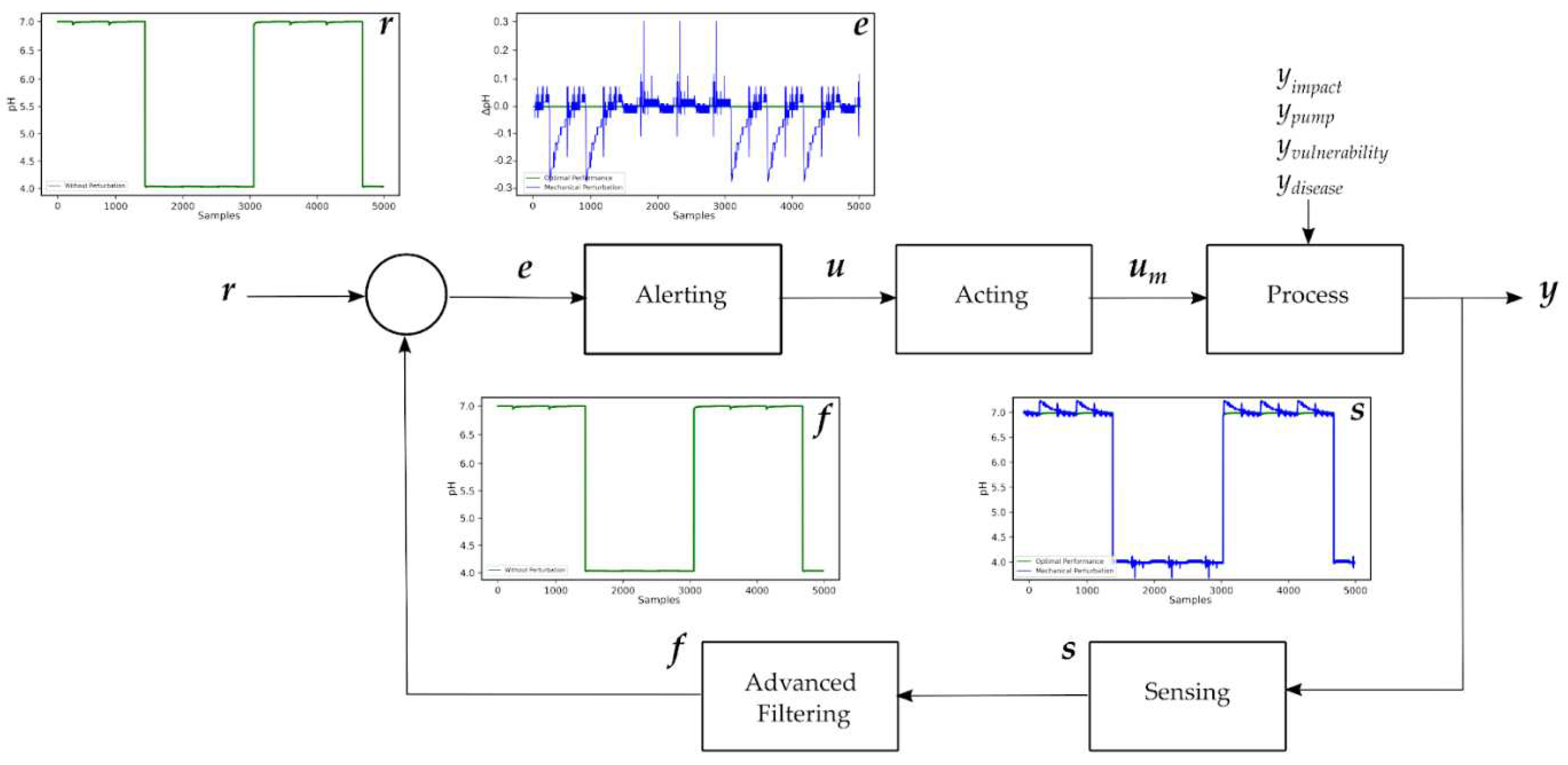
As commented above, controlling the pH, within a particular species-dependent range, is critical to ensure that the crop of interest will exhibit the expected yield, as well as being protected against plant vulnerability and diseases. Furthermore, real-life VF arrangements are bound to suffer mechanical perturbations that are unpredictable. Therefore, recurring to fundamental control theory, the challenge to ensure that a VF setup is exposed to appropriate pH values can be schematized as shown in
Figure 1.
The pH of a VF setup must be varied according to an
on-off cycle, in order to ensure sufficient (avoiding overabundance) nutrients are delivered to the VF arrangement. This implies that the pH input function is periodic with a rather slow varying frequency. For example, orchids and blueberries need to be exposed to pH values close to 4 units [
26,
27,
28,
29] for a period of 8 hours, while optimally resting for 8 hours (when the pH of the reference substance in the container can be neutral as shown in
Figure 1) before being exposed to another cycle. These application-dependent conditions enable us to predefine the expected waveforms (i.e., the reference signal,
r in
Figure 1) needed to enact the necessary control. However, as expected in any control system, perturbations occur, and it is of utmost importance to consider and address them appropriately.
As depicted in
Figure 1, four distinct perturbations are bound to occur in VF systems: 1. Extrinsic unpredictable mechanical perturbations,
yimpact, such as impacts; 2. Intrinsic random mechanical disturbances,
ypump, such as pump-induced effects; 3. Intrinsic crop vulnerabilities,
yvulnerability; and 4. Intrinsic crop diseases,
ydisease. The most challenging of these perturbations are the mechanical unpredictable ones. By implementing an Advanced Filtering stage, we demonstrate that such unpredictable behavior can be correctly addressed.
Two different types of digital filters exist: a. Fixed coefficient filters, including infinite impulse response (IIR) filters; and b. Variable coefficient filters, which include neural networks. Hereafter, we briefly present the theory of IIR filters (a cursory overview of digital filters has been recently reported in the literature, and newcomers are encouraged to refer to this material [
30]) and delve into more detail on the theory of recursive neural networks as pertinent to this work.
2.1. Infinite Impulse Response Filters
Extensive literature exists to introduce the theory of infinite impulse response (IIR) digital filters [
14,
15,
16,
17]. IIR digital filters can be described by means of their transfer function
H(z), as shown in Equation (1) [
31];
By rearranging, Equation (1) can be rewritten in the optimal form for inverse transformation,
Here, z is the z-space variable. Meanwhile, al and bk represent the IIR fixed filter coefficients. Additionally, M and N are the degrees of the numerator and denominator polynomials, respectively.
By setting the
a0 coefficient to unity, as conventionally done, and rearranging Equation (2), we obtain the filter output in the time domain by means of the inverse z-transform.
Finally, by determining the fixed coefficients of Equation (3), we can fully describe the output of arbitrary IIR digital filters.
2.2. Recurrent Neural Networks
Recurrent Neural Networks (RNNs) are artificial neural networks that differ from the most common Feedforward Neural Networks (FNNs) by introducing short memory effects, directional information cycles, and significant multicollinearity in the RNN variables, produced with weight connections between the same layer of neurons. RNNs add the possibility of changing the predicted behavior of the network depending on previous inputs. However, they are limited to short-time sequences because their updating gradients vanish or explode rapidly [
25].
2.2.1. Long Short-Term Memory Networks
Hochreiter and Schmidhuber proposed Long Short-Term Memory (LSTM) Networks in 1997. They have become the most popular RNNs. LSTMs predict long data sequences over a defined period, solving the vanishing problem in RNNs. An LSTM segment consists of blocks of cells. Each cell has its inputs, outputs, and memory. Cells that belong to the same block share input, output, and forget gates. The input gate decides whether the given information is worth remembering, and the forget gate decides how much of the given information is still worth remembering. The output gate decides whether the provided information is relevant at a given step. Each gate can be considered a neuron, and the LSTM cell is a hidden segment in a FNN [
32].
In order to perform advanced filtering for the feedback signal depicted in
Figure 1, we propose to suppress random pH perturbations (refer to signal
s in
Figure 1) with unpredictable behaviors for VF using neural networks. We perform such advanced filtering by utilizing the monitoring features of time sequences and of previous outputs that are characteristic of RNNs together with Deep Learning, aiming to obtain the response of the sensor (signal
f in
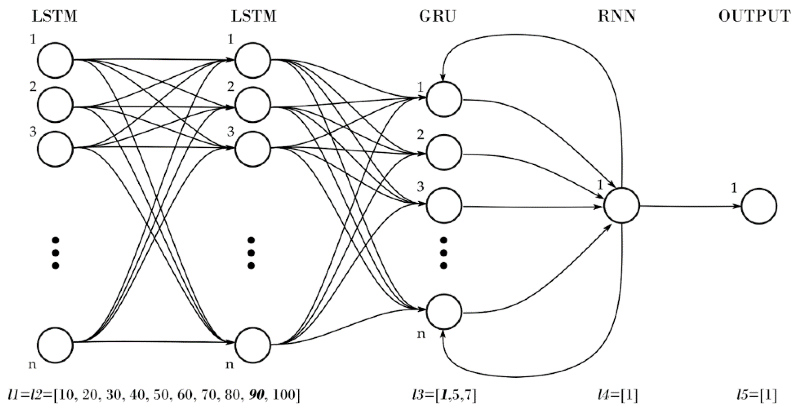
Figure 1) in the absence of unpredictable (mechanical) perturbations. As depicted in
Figure 2, the Deep-Learning model tested in this work has five layers with neurons used to design RNNs. The first and second segments,
l1 and
l2, only contain LSTM neurons, the third layer,
l3, contains Gated Recurrent Units (GRU) neurons, the fourth layer,
l4, contains simple RNN networks, and the final segment,
l5, is the output layer with a single neuron with a rectified linear activation function.
In the next section we present the materials used to generate the datasets, as well as the methods, such as filter designs including the frequency response of the IIR digital filters and the deep-learning RNN procedure, employed in this work.
3. Materials and Methods
3.1. Materials
3.1.1. Instrumentation
For the purpose of generating reference and output datasets (
r and
y in
Figure 1), we utilized the pH instrumentation recently reported by our group. The instrument is conformed of a potentiometric
silver|silver-chloride electrode (Hinotek, Ningbo, China, E201-BNC), which employs a dedicated electronic module (DIY More, Hong Kong, China PH-4502C) to detect the (analog) pH voltage signal. Signal digitization is achieved by a 10-bit ADC Arduino UNO (Smart projects, Ivrea, Italia, Arduino UNO), and the resulting (digital) pH voltage values are transmitted wirelessly by means of a Bluetooth (Olimex, Plovdiv, Bulgaria, BLE HC-06) radio [
13].
Once the data is received, the computing entity performs the IIR and RNN digital filtering. For IIR digital filtering, we employed the Signal Processing Toolbox of MATLAB (MathWorks, Natick, United States, MATLAB) running on a Windows 10 Dell G3 3500 computer with a 4-core Intel i5-10300H 2.50GHz processor with 16GB of RAM. The RNN analysis was performed with the TensorFlow, Sklearn, and other conventional python libraries of JupyterLab (NumFOCUS, Austin, United States, Jupyter) running on a Windows 10 Desktop Computer with an Intel i7-6700 3.40GHz processor with 16GB of RAM and NVIDIA GeForce RTX 2060 GPU.
3.2. Methods
Figure 3 displays (a) the block diagram and (b) the experimental setup that are needed to generate the training and testing waveforms, in order to assess the deep-learning RNN and IIR digital filters. The training dataset is created by using an ideal pH sensing setup without mechanical perturbations, see the central section of
Figure 3b. Meanwhile, the intrinsic mechanical perturbations are enacted by exposing the instrument to a laboratory stirrer, refer to the left section of
Figure 3b, which mimics the use of conventional pumps in VF systems for circulation purposes [
33,
34]. Finally, the extrinsic mechanical perturbations were created by impacting the utilized setup, at different locations, as depicted in the right-most portion of
Figure 3b.
3.2.1. Generation of Dataset
The objective of this study is to present a comparative analysis of advanced, RNN versus IIR, digital filters to optimize resilience to dynamic perturbations in pH sensing for VF applications. For this purpose, we need to generate the pH waveforms. Hereafter, we present the methodology followed to achieve this goal.
As reported recently by our group, to generate training and testing datasets, the instrumentation was first cleaned and calibrated. Reliable solutions (Mallinckrodt Baker, Hampton, New Jersey, USA) were utilized to ensure accurate pH values (
pHsignal = 3.99 and
pHreference = 6.98) for the measurements [
13].
We performed two sets of pH measurements for ideal and real scenarios, corresponding to mechanical perturbations being absent and present, respectively. In addition to pH values, we recorded the raw ADC temporal voltage values for redundancy and better control of the datasets. Thus, the dataset samples () included: input temporal indices, ti, ADC voltages, vi, and pH values, pHi, for (a) ideal and (b) real scenarios, for every sample . It is worth noting that the aforementioned datasets have a periodic behavior, in order to emulate the characteristic on-off cycle necessary to ensure optimal crop growth and yield.
3.2.2. Dataset Augmentation and Splitting
Specifically with respect to the RNN analysis, we utilized both datasets to train the model and suppress perturbations. As depicted in
Figure 2, the RNN is based on a supervised-learning model, which requires knowledge of the input signals, as well as the desired output for training purposes. Since after RNN filtering, we are interested in obtaining pH signals free of perturbations, we solely utilized the signal without perturbations as the desired output dataset to train the model. Thus, the training input and output datasets were
and
, where
and
were pH values for the signals with perturbations and without them, respectively.
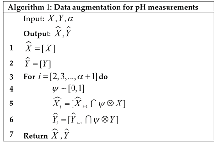
Furthermore, we employed a data augmentation mechanism to increase the dataset samples and the representativity without the need for new measurements. The data augmentation in this work considered that the pH instrumentation will record values in the range 0-14, depending on the level of acidity or alkalinity of the solution. We commenced the data augmentation by selecting a, the number of augmentations. Then, for each augmentation, we determined a random value in the range of to multiply by the original and , equally modifying the pH values while maintaining the result within the original boundaries . Finally, we maintained the original samples and added each augmentation to return the augmented data and , as detailed in Algorithm 1. It is important to note that we employed 30 augmentations of the entire training dataset, or , and that the augmented dataset can also be employed to test the IIR filters.

Considering that we must train a deep-learning neural network, the dataset must be split to avoid overfitting and to ensure reliable results. In this work, we utilized 60% of the dataset for training, 20% for validation, and 20% for testing. Thereafter, we configured the model to generate extra data with the training augmentation data, as described in Algorithm 1.
3.2.3. Training Datasets
The pH values utilized to assess the performance of RNN and IIR digital filters were 4 and 7 units for signal and reference waveforms, respectively. However, before commencing pH measurements, the instrument must be calibrated[
13]. Thus, for calibration purposes, we included a third pH value of 10.00 of a standardized buffer solution (Mallinckrodt Baker, Hampton, New Jersey, USA). Finally, the calibration procedure can be improved if a fourth solution, outside of the calibrated substance range in our case [3.99, 10.00], is utilized. Hence, a final substance of 2.5 pH units was employed to perform the calibration procedure. Thereafter, the periodic signal needed for VF was generated.
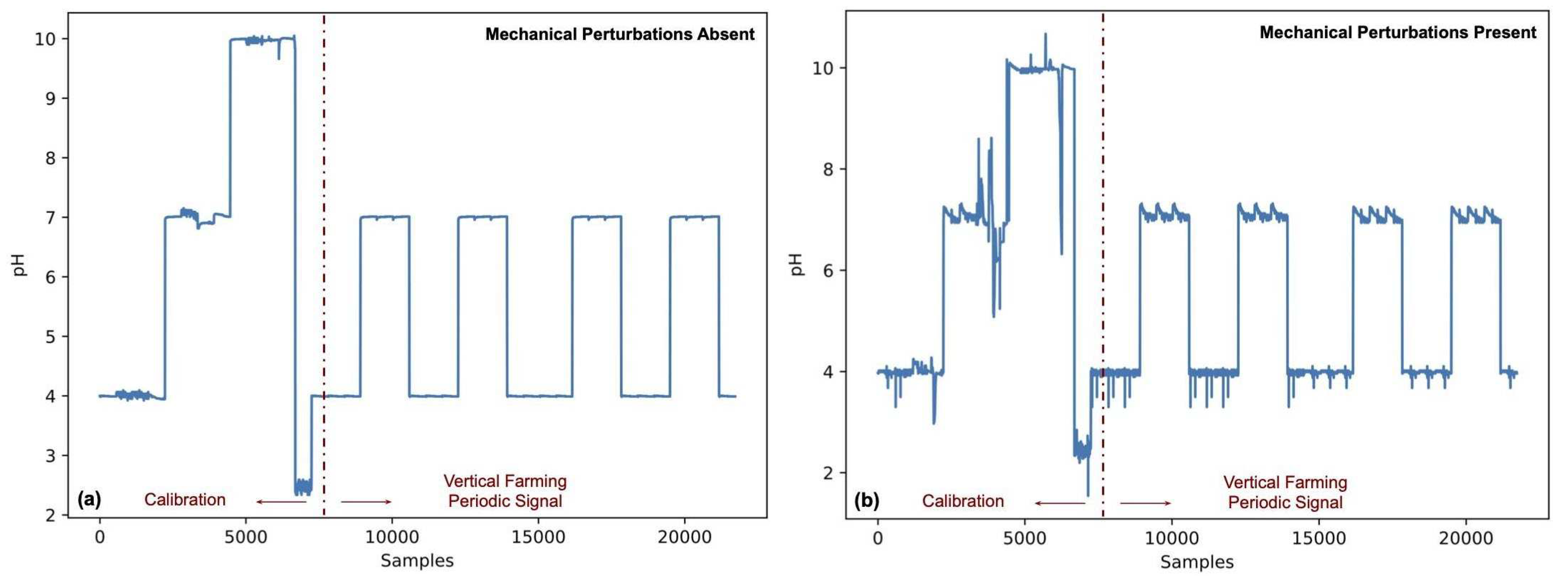
Figure 4 depicts the training dataset (a) without mechanical perturbations, and (b) with intrinsic and extrinsic disturbances. Moreover, in
Figure 4, we separate into two phases the required steps, calibration and measurement, needed to sense pH with the portable instrumentation. The datasets consisting of 21723 temporal samples,
ti, ADC voltages,
vi, and pH values,
pHi, for scenarios with present and absent perturbations are available in the
Supplementary Materials section of this work.
As seen in
Figure 4, once the instrument is duly calibrated, we generate the periodic signals, which are identical to the control waveforms of
Figure 2. During calibration, the instrument is more prone to exhibit mechanical perturbations because buffer solution, electrode, and detection electronics have to be manipulated frequently (i.e., electrode and container cleaning is mandatory after each calibration measurement). In this work, we consider these unpredictable fluctuations to demonstrate that a RNN filter is more resilient in real scenarios, as opposed to IIR filtering.
3.2.4. IIR Digital Filter Designs
The portable and precise pH instrument that we recently proposed can implement well-established (analog or digital) electronic filters, such as Butterworth, Chebyshev, and Elliptic arrangements. Furthermore, a salient feature of IIR filters is that they can be based on these electronic configurations. In order to assess the usability of such filters in real-life VF applications, we designed (a) Butterworth, (b) Chebyshev I, (c) Chebyshev II, and (d) Elliptic digital IIR configurations. As commented previously, the pH input function is periodic with a rather slow varying frequency. Therefore, the low-pass filters specifications have to consider this expected behavior. We defined a passband frequency of 1Hz with a maximum 1dB attenuation. Additionally, the stopband frequency was specified to be 10Hz for a 60dB attenuation. The sampling frequency was assumed to be one order of magnitude greater than the stopband frequency.
Utilizing the Signal Processing Toolbox of
MATLAB, we determined filter orders, as well as the corresponding transfer functions of the filters, including the
a and
b coefficients of Equation (2).
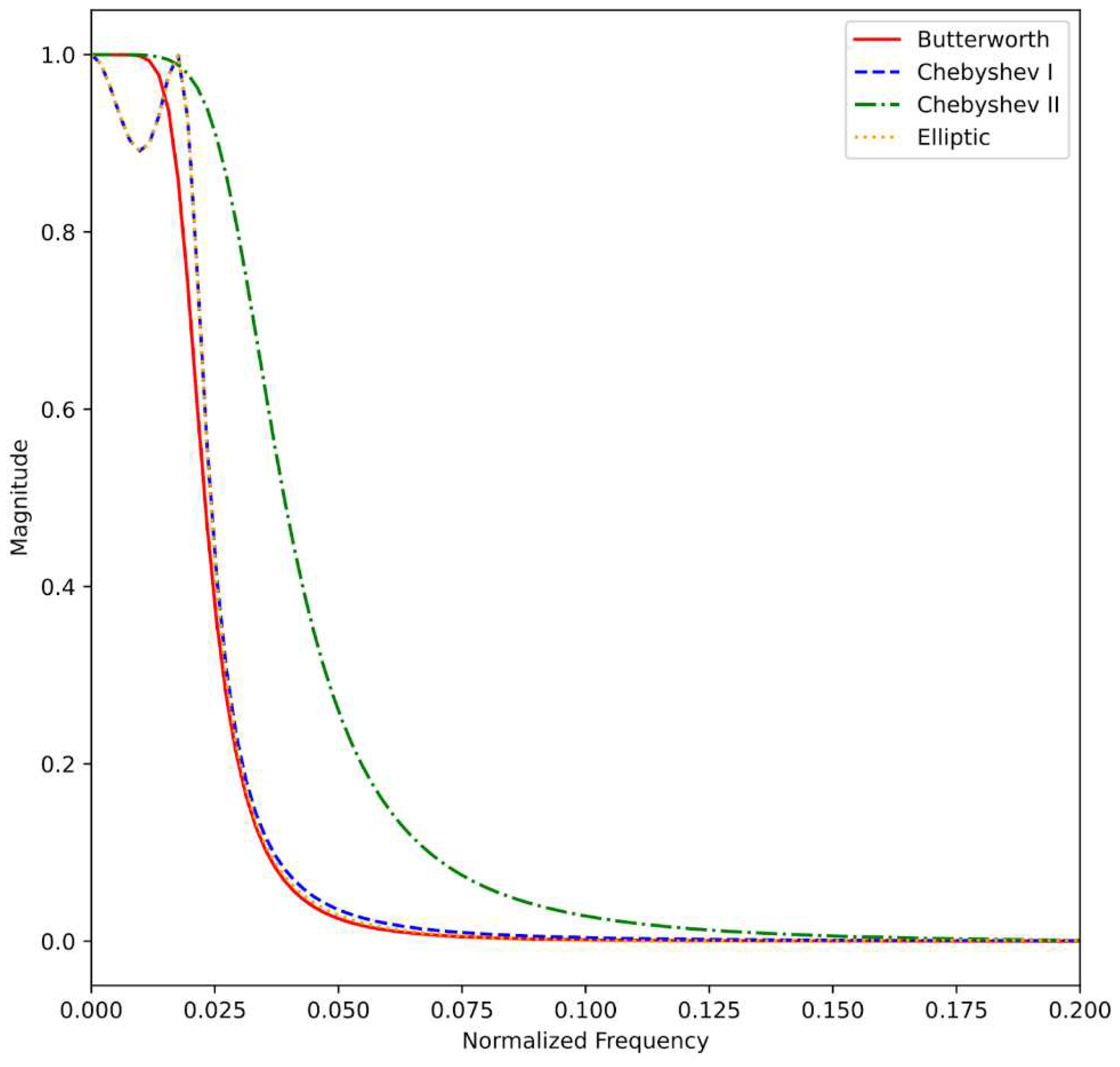
Table 1 presents the orders, coefficients, and transfer functions of the digital filters. Finally,
Figure 5 illustrates the digital filter designs for (a) Butterworth, (b) Chebyshev I, (c) Chebyshev II, and (d) Elliptic digital IIR configurations. The IIR digital filter
MATLAB scripts are available in the
Supplementary Materials section of this work.
3.2.5. RNN Digital Filter Design
The RNN-based digital filter proposed in this work implements the advanced structure depicted in
Figure 2. In order to optimize the design of the RNN digital filter, we determined the number of neurons per layer by testing multiple configurations. The tested layouts included various
LSTM neurons; three different
GRU arrangements; as well as single RNN and output segments,
and
. Furthermore, we also varied the number of prior samples. We tested
. We assessed 2101 different configurations of the model with the MSE loss function, which we decided to employ because it is the most utilized metric to train regression models in ANNs [
35]. For the 2101 configurations, we trained the model with 500 epochs and a batch size of 5000. This approach requires different steps per epoch depending on the size of the training set, which is variable because, as commented above, we allowed changing the prior samples required as inputs. Moreover, we adjusted the learning rate according to Equation (4), increasing the effect of error and modifying the learning rate across epochs.
The training mechanism utilized in this work stops after twenty steps without improvement of the validation loss. Furthermore, we configured the training process to solely save the best model. After assessing the 2101 configurations with the dataset containing 21723 samples with 30 augmentations for training, we obtained that the best model, as determined by the MSE loss function, ensues when
,
,
,
,
, and
. In
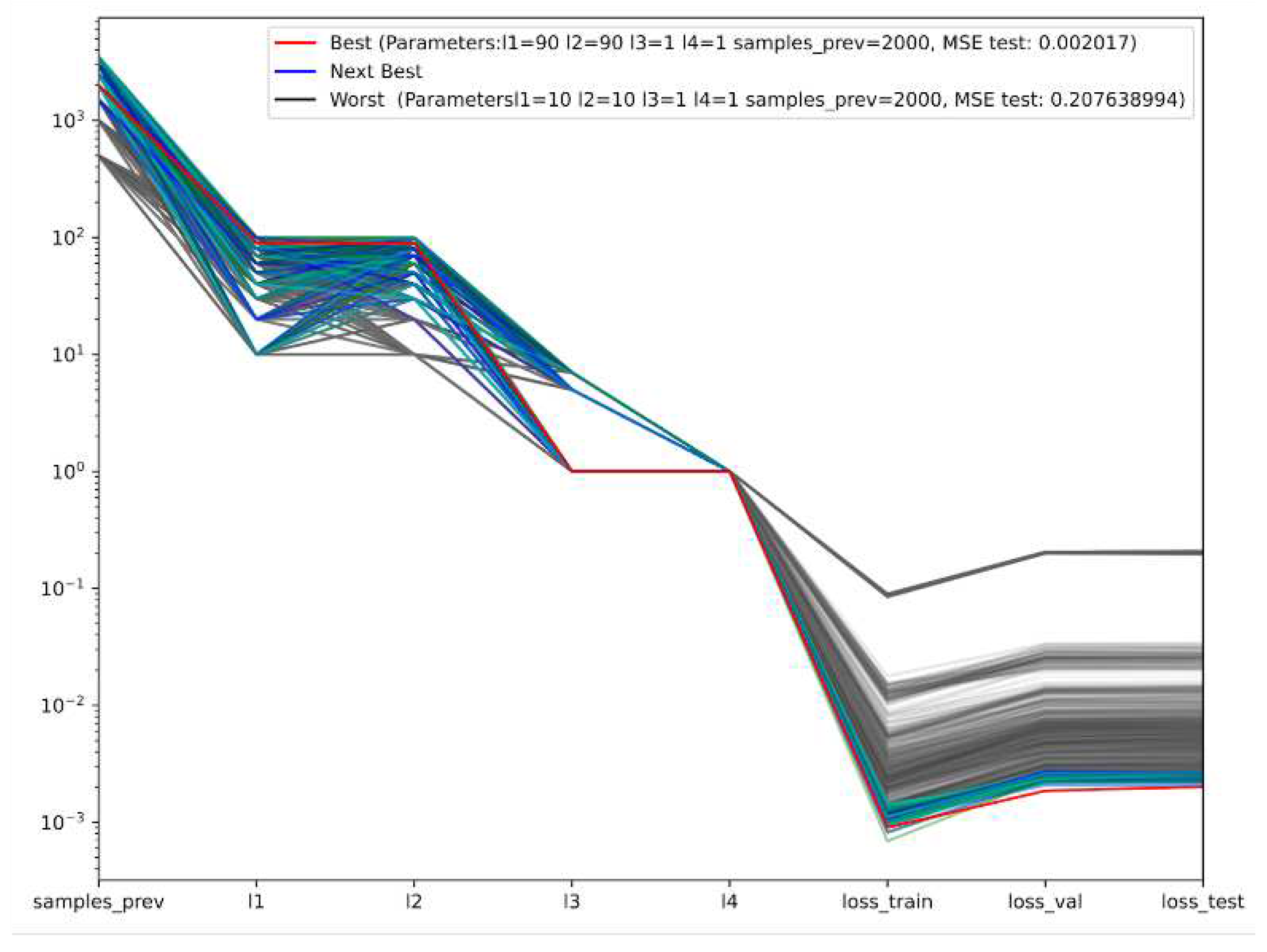
Figure 6, we depict the logarithmic parallel coordinates for all the configurations trained with the MSE loss function based on the testing of MSE results. The best model is highlighted in red,
MSE Test = 0.002017. Meanwhile, blue and gray are variations of models exhibiting better and worse performance, respectively. Lastly, in black we present the model with the worst outcome,
MSE Test = 0.207638994.
The training metrics obtained for the best model trained with the MSE loss function at the maximum step reached before stopping due to no loss validation improvement are depicted in
Table 2.
The validation metrics for the best model trained with the MSE loss function obtained at the maximum stage reached are enumerated in
Table 3.
The test metrics obtained for the best model trained with the MSE loss function are enlisted in
Table 4.
Once the digital filters were fully characterized, we assessed their implementation in a VF setting, as described next.
4. Results
In real-life VF settings, the pH instrument will be calibrated and utilized to generate periodic signals exhibiting unpredictable patterns depending on multiple factors. Thus, the expected output of a pH instrument should include both phases, although the most prevalent one will be the periodic one. We utilized the waveforms of
Figure 4 to quantify the performance of IIR and RNN digital filters for VF applications.
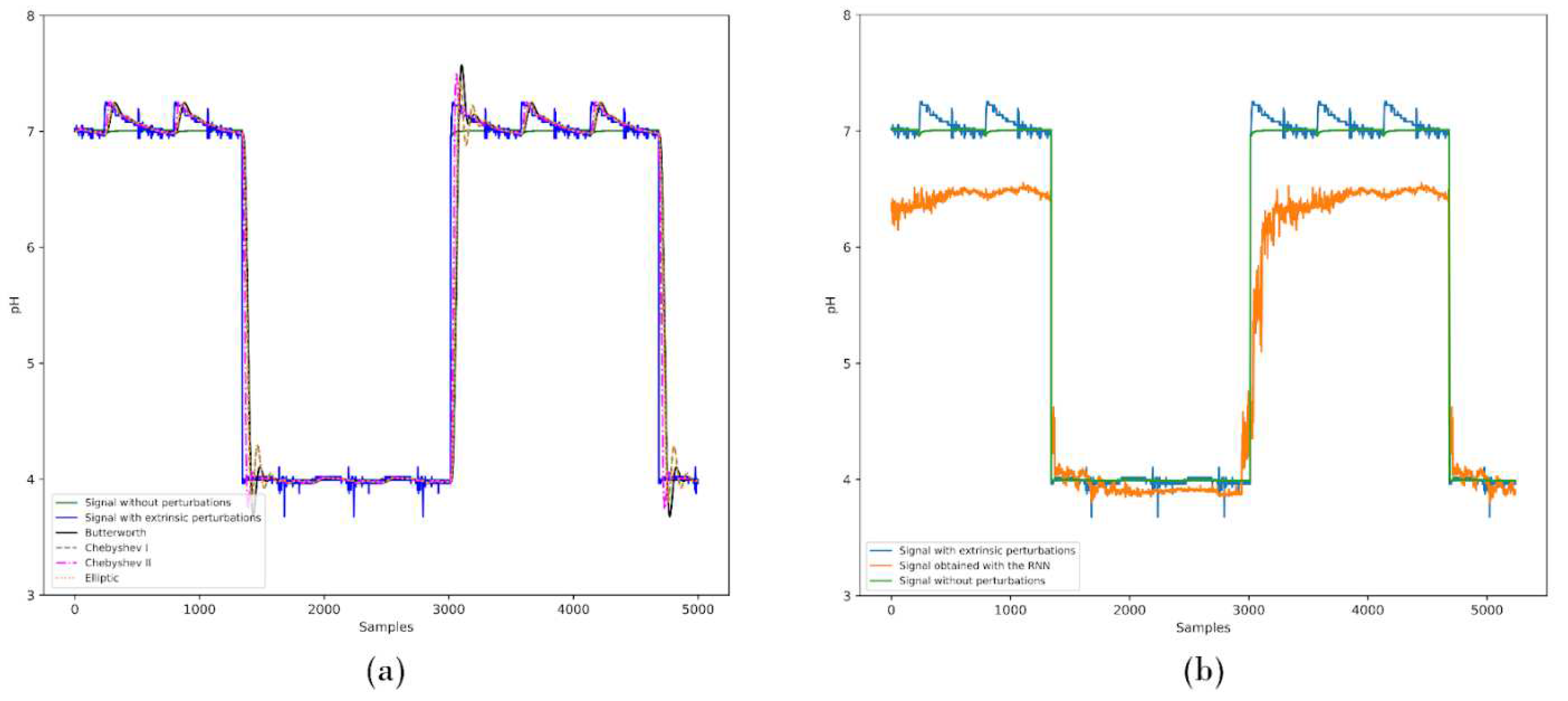
We commenced our assessment of both sets of digital filters by utilizing as test waveforms those of extrinsic (mechanical) perturbations enacted by impacting the container. Hereafter, we present the data with perturbations, without disturbances, and the output of the IIR models
, as well as the RNNs trained model to filter the perturbations. In
Figure 7, we show the obtained results for (a) IIR and (b) RNN.
The test metrics obtained for the IIR and the best trained RNN digital filters, employing the MSE loss function, while exposed to extrinsic mechanical perturbations, are enlisted in
Table 5.
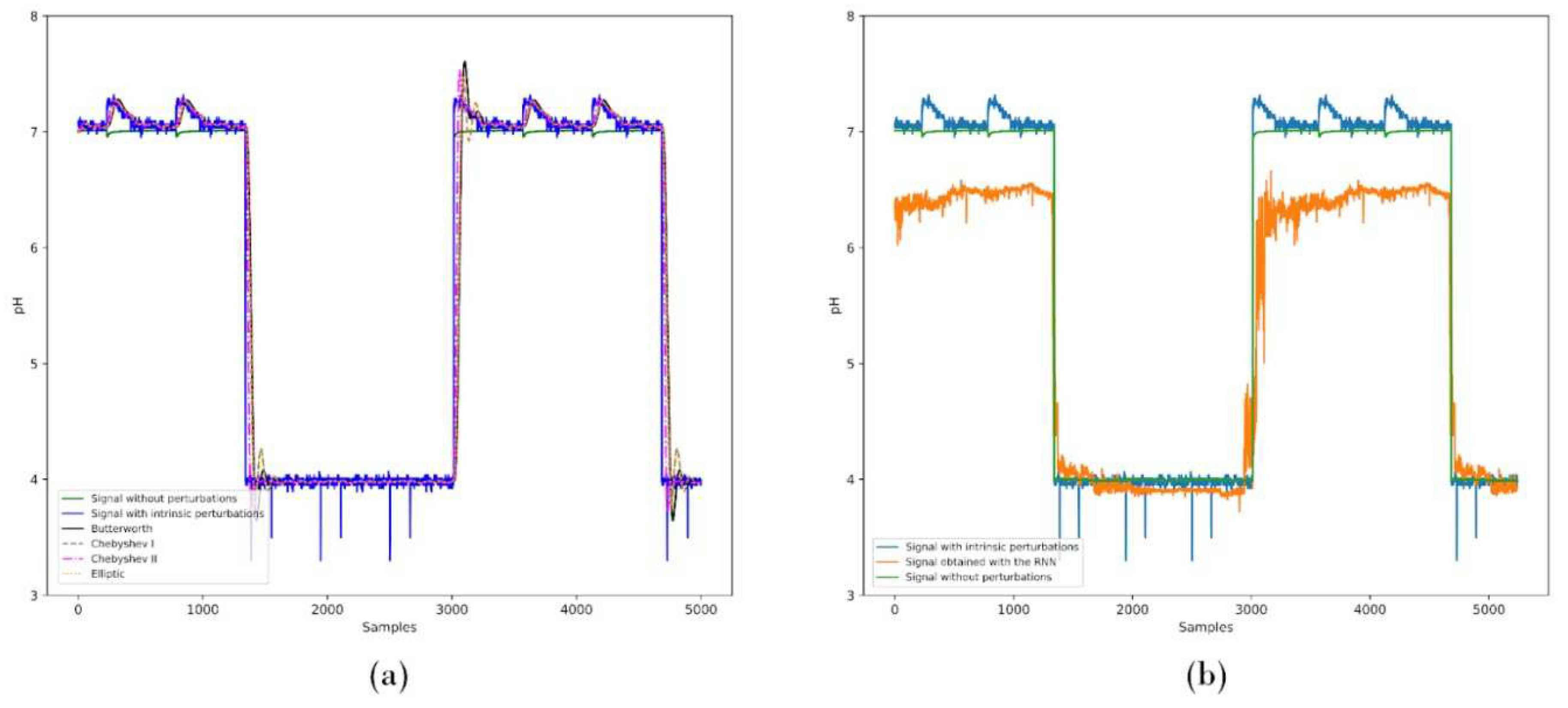
We continued the analysis by using as test signals the waveform of intrinsic perturbations, generated by means of the mechanical stirrer (refer to
Figure 3), which mimics the recurrent pump variations encountered in VF settings. In
Figure 8, we depict the results of the IIR and RNN models when exposed to intrinsic perturbations. In turn, in
Table 6 we present the loss function MSE evaluation for IIR and RNN models as applicable to intrinsic disturbance.
Continuing our analysis of the advanced digital filter based on the RNN model described in this work, we assessed the extrinsic, i.e.,
Figure 7b and
Table 5, as well as the intrinsic, i.e.,
Figure 8b and
Table 6, mechanical perturbation results to determine if the RNN model performance could be improved by utilizing a rescaling constant,
k. Thus, we returned to the training dataset and optimized a scaling parameter,
k, in ranges
with steps of 0.001 (500 tests), multiplying the model output to improve the
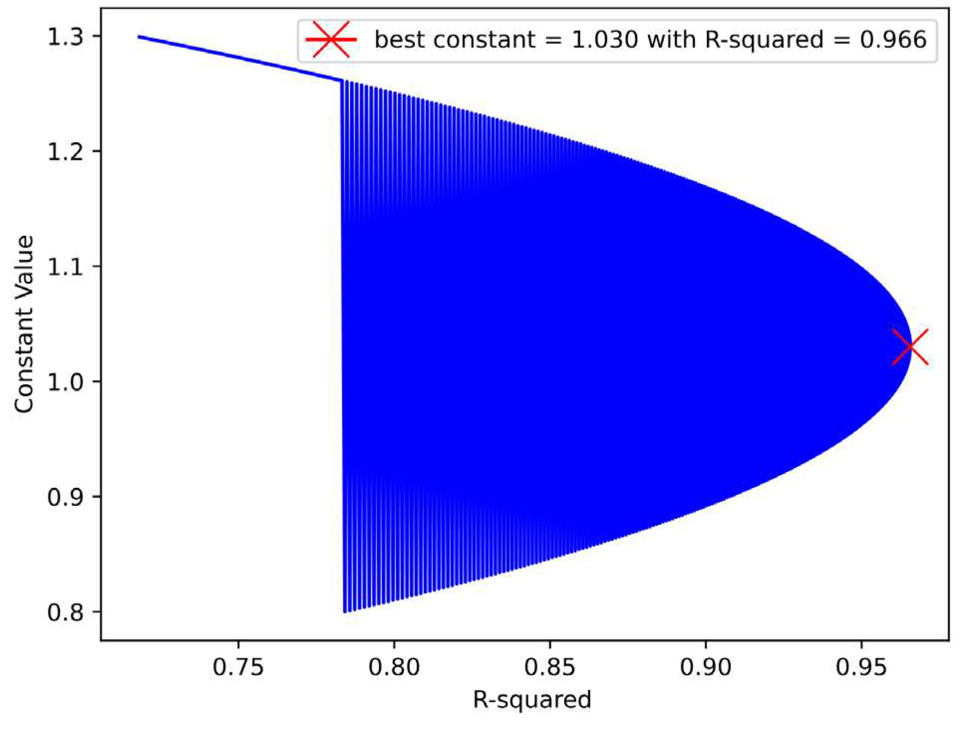
R-squared metric without changing the previously trained model. The obtained constant was
k = 1.030, as shown in the optimization results of
Figure 9. Using the aforementioned constant, we computed again the test metrics obtained for the test dataset in the best model trained with the MSE loss function but now using the output scaling constant. The corresponding results are depicted in the last entry of
Table 4.
Thereafter, we tested the scaled RNN, in short
k-RNN, digital filter employing the extrinsic mechanical perturbations. Furthermore, in order to remove the harmonic oscillations of the
k-RNN digital filter, we applied a moving average filter (MAF) with 300 samples to obtain the output waveform.
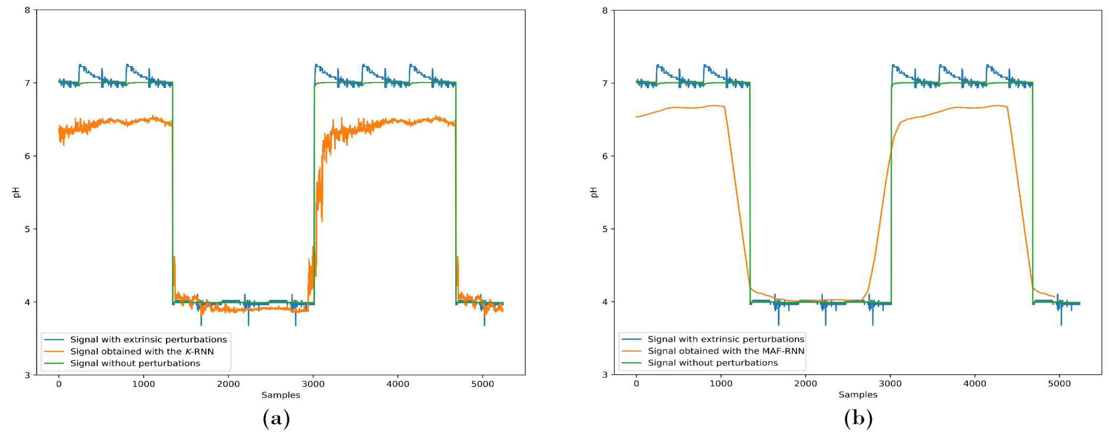
Figure 10 depicts the results obtained for (a)
k-RNN and (b) MAF-RNN digital filters while exposed to waveforms with extrinsic perturbations. In
Table 5, we demonstrate that an
R-squared metric of 0.9302 is obtained for the
k-RNN model when exposed to unpredictable extrinsic mechanical perturbations.
Finally, we calculated the
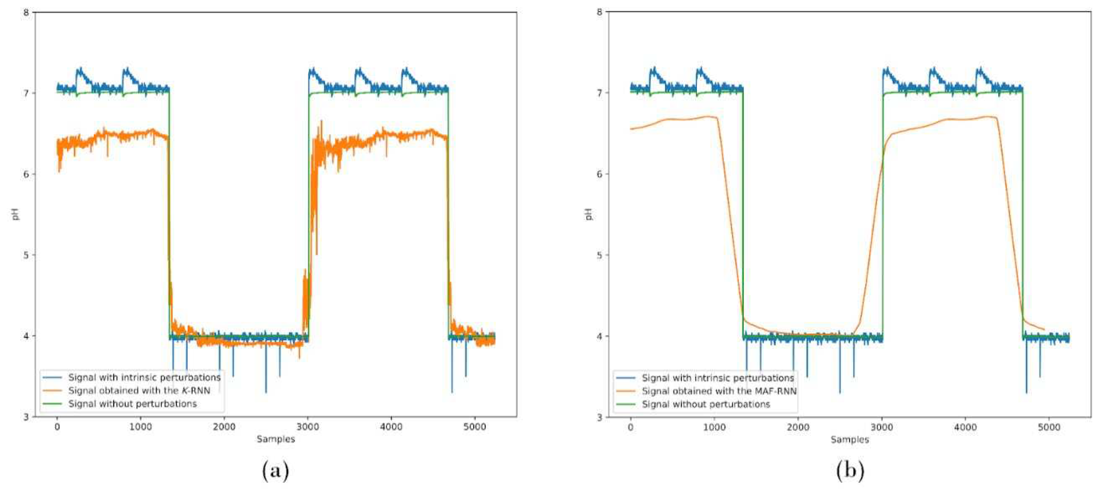
k-RNN and MAF-RNN digital filter performance when exposed to intrinsic mechanical perturbations. In
Figure 11, we show the digital filtering performance for (a)
k-RNN and (b) MAF-RNN models when exposed to waveforms with intrinsic perturbations. The corresponding test metrics when exposing the
k-RNN filter to intrinsic mechanical perturbations are illustrated in the last entry of
Table 6.
In the next section, we discuss the results and demonstrate how the RNN digital filter can be tuned to suit other VF applications.
5. Discussion and Future Work
In real-life VF settings, unpredictable mechanical perturbations hinder the implementation of efficient control strategies. Furthermore, as shown in this work, the use of conventional IIR digital filters introduces unwanted oscillations, which would impede the control process. Thus, the construction of robust solutions to address the filtering challenge is of utmost importance.
In this work, we have focused on providing an advanced digital filtering scheme based on RNN. As depicted in
Figure 1, we assessed the RNN schemes for a signal centered at 4 pH units, while the reference signal was centered at 7. As commented before, such a configuration is pertinent to grow orchids and blueberries, pH ~4, and to maintain the electrode in good condition with a reference substance (in
Figure 1 reference pH ~7, representative of water) whilst not administering nutrients.
The filtered signals,
f in
Figure 1, obtained with the RNN schemes, and depicted in
Figure 7b,
Figure 8b,
Figure 10, and
Figure 11 share several important features. First, we tuned the design of the RNN, including the multiplicative constant, to accurately filter the nutrition signal; centered at pH ~4. Second, the RNN signals do not exhibit considerable lags, which is relevant to avoid overexposing (i.e., to control) the crop to the nutrient substance. With respect to this last feature, it is worth noting that by modifying the MAF window size, we can control the lag exhibited in
Figure 10b and
Figure 11b.
A salient feature of our RNN scheme has to do with the tuning of the digital filter. It is widely known that many crops require a nutrient substance with a pH close to 7 units [
36,
37]. A set of representative crops needing a pH close to 7 include lettuce, tomatoes, spinach, eggplants, and more [
38]. Hereafter, we present a modification of the RNN proposal to suit a signal centered close to 7 units, whilst assuming the reference pH is close to 4.
The RNN performance can be tuned by modifying the optimization constant, k. As before, we optimized the constant utilizing the R-squared metric with the signal dataset.
This yields a particularly flexible digital filtering approach, because the constant does not change the behavior of the RNN model, rather it serves to tune the RNN to tackle different specific challenges. We performed an optimization procedure similar to the one shown in
Figure 9 and obtained new values for optimization constant and
R-squared metrics; namely
k = 1.076 and
R-squared = 0.959.
Afterwards, we tested the newly scaled
k-RNN digital filter, assuming the same configuration of the MAF to eliminate harmonic oscillations of the output waveforms.
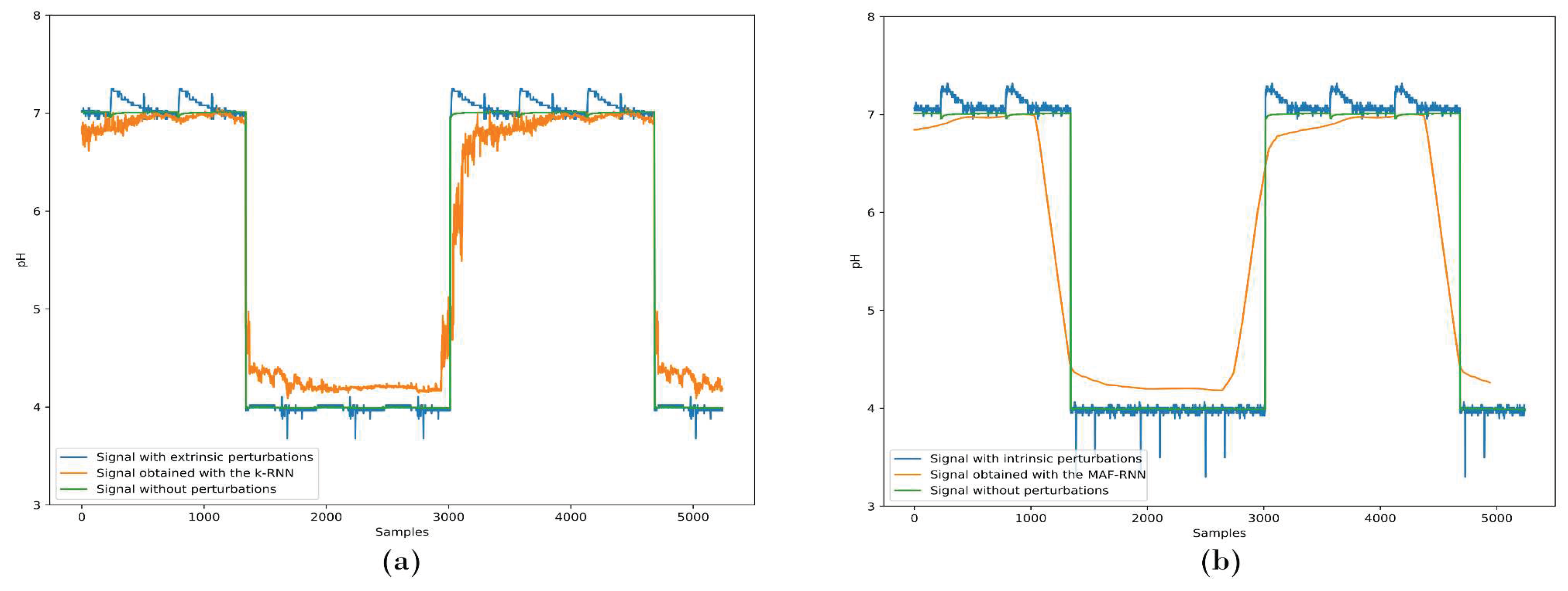
Figure 12 depicts the results obtained for the
k-RNN and MAF-RNN digital filters, tuned for a different pH value (i.e., at a particular constant k = 1.076), while exposed to waveforms with (a) extrinsic and (b) intrinsic perturbations.
As demonstrated in
Figure 12, the RNN-based digital filters are particularly flexible for VF applications. Once the neural network has been adequately trained, we may tune the performance of the RNN digital filter by selecting the signal (i.e., pH) of interest. In a real VF setting, this feature is rather important because we can enact selective control depending on the crop of interest, without the need to re-train the neural network.
In the future, we will extend the analysis of the RNN model presented here to include the effects of vulnerability and disease in the detected signal. As commented before, both of these factors are critical to determine crop growth and yield.
6. Summary
In this work, we have proposed an advanced filtering scheme based on Recurrent Neural Networks (RNNs) and Deep Learning to enable efficient control strategies for Vertical Farming (VF) applications. We demonstrated that the best RNN model incorporates five neuron layers. The first and second of the segments contain ninety LSTM neurons. The third layer implements one GRU neuron. The fourth segment incorporates one RNN network, while the output layer was designed by using a single neuron exhibiting a rectified linear activation function. By utilizing this RNN digital filter two variations were introduced: (1) A scaled RNN model to tune the filter to the signal(s) of interest, and (2) A moving average filter to eliminate harmonic oscillations of the output waveforms. The RNN models were contrasted with conventional Butterworth, Chebyshev I, Chebyshev II, and Elliptic digital IIR configurations. The RNN digital filtering schemes avoid introducing unwanted oscillations, which makes them more suitable for VF than their IIR counterparts. Furthermore, by utilizing the advanced features of scaling of the RNN model, we demonstrated that the RNN digital filter is pH selective, as opposed to conventional IIR filters. In real VF settings, the features of tuning (or selecting) an instrument to detect variable pH values, as well as ensuring that such device is resilient to dynamic (i.e., unpredictable) perturbations are of utmost importance. Hence, the use of advanced filtering schemes such as those based on RNN and Deep Learning is preferable as opposed to employing IIR filtering for VF.
Author Contributions
Conceptualization, R.H.-M., M.M.R., P.V.-J. and N.E.-G.; Methodology, M.M.R., P.V.-J. and E.O.-G.; Software, R.H.-M., M.M.R., P.V.-J. and A.B.S.; Validation, R.H.-M., A.B.S. and E.O.-G.; formal analysis, R.H.-M., M.M.R., P.V.-J. and N.E.-G.; investigation, R.H.-M., N.E.-G., J.A.D.-A. and A.B. S.; resources, M.M.R., P.V.-J., N.E.-G. and E.O.-G.; data curation, R.H.-M., M.M.R., P.V.-J. and J.A.D.-A. writing—original draft preparation, R.H.-M., M.M.R., P.V.-J. and N.E.-G.; writing—review and editing, all authors; visualization, R.H.-M., P.V.-J., N.E.-G., J.A.D.-A. and A.B.S.; supervision, P.V.-J., N.E.-G. and E.O.-G.; project administration, M.M.R., P.V.-J., N.E.-G. and J.A.D.-A.; funding acquisition, J.A.D.-A., A.B.S. and E.O.-G. fund raising, E.O.-G. and N.E.-G. All authors have read and agreed to the published version of the manuscript.
Funding
We acknowledge the support of the Consejo Nacional de Ciencia y Tecnología (CONACYT) in Mexico for supporting this work through funds for projects INFRA-2016-01, Project No. 270665. CB-2016-01, Project No. 287818. Additionally, we acknowledge the support to the Government of the State of Aguascalientes, and the Instituto para el Desarrollo de la Sociedad del Conocimiento del Estado de Aguascalientes (IDSCEA) through the Technological Innovation Fund.
Institutional Review Board Statement
Not applicable.
Informed Consent Statement
Not applicable.
Data Availability Statement
Not applicable.
Conflicts of Interest
The authors declare no conflict of interest.
References
- FOOD SECURITY AND NUTRITION IN THE WORLD THE STATE OF REPURPOSING FOOD AND AGRICULTURAL POLICIES TO MAKE HEALTHY DIETS MORE AFFORDABLE. 2022. [CrossRef]
- Hurst, W.; Mendoza, F.R.; Tekinerdogan, B. Augmented Reality in Precision Farming: Concepts and Applications. Smart Cities 2021, Vol. 4, Pages 1454-1468 2021, 4, 1454–1468. [Google Scholar] [CrossRef]
- Raj, E.F.I.; Appadurai, M.; Athiappan, K. Precision Farming in Modern Agriculture. 2021, 61–87. [CrossRef]
- Li, H.; Yang, H.; Zhan -, M.; Haruyama, S.; Darmawan, Z.; Kaminishi -, K.; Zheng, Y.; Yang, M.; Yao, L.; Chengming, L.; et al. Analysis on Water Wall Tube Explosion in a Power Plant. IOP Conf Ser Earth Environ Sci 2020, 526, 012162. [Google Scholar] [CrossRef]
- Van Gerrewey, T.; Boon, N.; Geelen, D. Vertical Farming: The Only Way Is Up? Agronomy 2022, Vol. 12, Page 2 2021, 12, 2. [Google Scholar] [CrossRef]
- Yin, H.; Cao, Y.; Marelli, B.; Zeng, X.; Mason, A.J.; Cao, C. Soil Sensors and Plant Wearables for Smart and Precision Agriculture. Advanced Materials 2021, 33, 2007764. [Google Scholar] [CrossRef] [PubMed]
- Msimbira, L.A.; Smith, D.L. The Roles of Plant Growth Promoting Microbes in Enhancing Plant Tolerance to Acidity and Alkalinity Stresses. Front Sustain Food Syst 2020, 4, 106. [Google Scholar] [CrossRef]
- Penn, C.J.; Camberato, J.J. A Critical Review on Soil Chemical Processes That Control How Soil PH Affects Phosphorus Availability to Plants. Agriculture 2019, Vol. 9, Page 120 2019, 9, 120. [Google Scholar] [CrossRef]
- Liming Effects on Soil PH and Crop Yield Depend on Lime Material Type, Application Method and Rate, and Crop Species: A Global Meta-Analysis Available online:. Available online: https://agris.fao.org/agris-search/search.do?recordID=US201900294097 (accessed on 19 April 2023).
- Adesina, I.; Bhowmik, A.; Sharma, H.; Shahbazi, A. A Review on the Current State of Knowledge of Growing Conditions, Agronomic Soil Health Practices and Utilities of Hemp in the United States. Agriculture 2020, Vol. 10, Page 129 2020, 10, 129. [Google Scholar] [CrossRef]
- Neina, D. The Role of Soil PH in Plant Nutrition and Soil Remediation. Appl Environ Soil Sci 2019, 2019. [Google Scholar] [CrossRef]
- Chandra, S.; Bhattacharya, J. Influence of Temperature and Duration of Pyrolysis on the Property Heterogeneity of Rice Straw Biochar and Optimization of Pyrolysis Conditions for Its Application in Soils. J Clean Prod 2019, 215, 1123–1139. [Google Scholar] [CrossRef]
- Hinojosa-Meza, R.; Olvera-Gonzalez, E.; Escalante-Garcia, N.; Dena-Aguilar, J.A.; Montes Rivera, M.; Vacas-Jacques, P. Cost-Effective and Portable Instrumentation to Enable Accurate PH Measurements for Global Industry 4.0 and Vertical Farming Applications. Applied Sciences 2022, Vol. 12, Page 7038 2022, 12, 7038. [Google Scholar] [CrossRef]
- Rader, C.M.; Gold, B. Digital Filter Design Techniques in the Frequency Domain. Proceedings of the IEEE 1967, 55, 149–171. [Google Scholar] [CrossRef]
- Pilipović, R.; Risojević, V.; Bulić, P. On the Design of an Energy Efficient Digital IIR A-Weighting Filter Using Approximate Multiplication. Sensors 2021, Vol. 21, Page 732 2021, 21, 732. [Google Scholar] [CrossRef] [PubMed]
- Dilmi, S. Calcium Soft Sensor Based on the Combination of Support Vector Regression and 1-D Digital Filter for Water Quality Monitoring. Arab J Sci Eng 2022. [Google Scholar] [CrossRef]
- Stanciu, L.; Stanciu, V.; Badea, R. Digital Filters with Small Transition Frequency Bands. ISSCS 2019 - International Symposium on Signals, Circuits and Systems 2019. [CrossRef]
- Ruospo, A.; Sanchez, E. On the Reliability Assessment of Artificial Neural Networks Running on AI-Oriented MPSoCs. Applied Sciences 2021, Vol. 11, Page 6455 2021, 11, 6455. [Google Scholar] [CrossRef]
- Sahu, S.K.; Mokhade, A.; Bokde, N.D. An Overview of Machine Learning, Deep Learning, and Reinforcement Learning-Based Techniques in Quantitative Finance: Recent Progress and Challenges. Applied Sciences 2023, Vol. 13, Page 1956 2023, 13, 1956. [Google Scholar] [CrossRef]
- Kim, T.; Vecchietti, L.F.; Choi, K.; Lee, S.; Har, D. Machine Learning for Advanced Wireless Sensor Networks: A Review. IEEE Sens J 2021, 21, 12379–12397. [Google Scholar] [CrossRef]
- Jospin, L.V.; Laga, H.; Boussaid, F.; Buntine, W.; Bennamoun, M. Hands-On Bayesian Neural Networks - A Tutorial for Deep Learning Users. IEEE Comput Intell Mag 2022, 17, 29–48. [Google Scholar] [CrossRef]
- Kimmel, J.C.; McDole, A.D.; Abdelsalam, M.; Gupta, M.; Sandhu, R. Recurrent Neural Networks Based Online Behavioural Malware Detection Techniques for Cloud Infrastructure. IEEE Access 2021, 9, 68066–68080. [Google Scholar] [CrossRef]
- Bendarkar, D.; Somase, P.; Rebari, P.; Paturkar, R.; Khan, A. Web Based Recognition and Translation of American Sign Language with CNN and RNN. International Journal of Online and Biomedical Engineering (iJOE) 2021, 17, 34–50. [Google Scholar] [CrossRef]
- Kang, T.; Lim, D.Y.; Tayara, H.; Chong, K.T. Forecasting of Power Demands Using Deep Learning. Applied Sciences 2020, Vol. 10, Page 7241 2020, 10, 7241. [Google Scholar] [CrossRef]
- Yang, D.; Gu, C.; Zhu, Y.; Dai, B.; Zhang, K.; Zhang, Z.; Li, B. A Concrete Dam Deformation Prediction Method Based on Lstm with Attention Mechanism. IEEE Access 2020, 8, 185177–185186. [Google Scholar] [CrossRef]
- Tasnim, R.; Calderwood, L.; Tooley, B.; Wang, L.; Zhang, Y.J. Are Foliar Fertilizers Beneficial to Growth and Yield of Wild Lowbush Blueberries? Agronomy 2022, Vol. 12, Page 470 2022, 12, 470. [Google Scholar] [CrossRef]
- Song, X.; Li, Y.; Hu, Y.; Guo, W.; Wu, Z.; Zhang, Y.; Cao, Z. Endophytes from Blueberry Roots and Their Antifungal Activity and Plant Growth Enhancement Effects. Rhizosphere 2021, 20. [Google Scholar] [CrossRef]
- Sopalun, K.; Iamtham, S. Evaluation and Optimization of Pectinase Production by Endophytic Fungi Isolated from Thai Orchids Using Agrowaste Medium. Journal of ISSAAS (International Society for Southeast Asian Agricultural Sciences) 2020, 26, 86–98. [Google Scholar]
- Schreiber, M.J.; Nunez, G.H. Calcium Carbonate Can Be Used to Manage Soilless Substrate Ph for Blueberry Production. Horticulturae 2021, 7, 74. [Google Scholar] [CrossRef]
- de Cheveigné, A.; Nelken, I. Filters: When, Why, and How (Not) to Use Them. Neuron 2019, 102, 280–293. [Google Scholar] [CrossRef] [PubMed]
- Borges, V.S.; Nepomuceno, E.G.; Duque, C.A.; Butusov, D.N. Some Remarks about Entropy of Digital Filtered Signals. Entropy 2020, Vol. 22, Page 365 2020, 22, 365. [Google Scholar] [CrossRef] [PubMed]
- Hossain, G.M.S.; Rashid, Md.H.O.; Islam, Md.R.; Sarker, A.; Yasmin, Must. A.; Hossain, G.M.S.; Rashid, Md.H.O.; Islam, Md.R.; Sarker, A.; Yasmin, Must.A. Towards Mining Public Opinion: An Attention-Based Long Short Term Memory Network Using Transfer Learning. Journal of Computer and Communications 2022, 10, 112–131. [Google Scholar] [CrossRef]
- Vatistas, C.; Avgoustaki, D.D.; Bartzanas, T. A Systematic Literature Review on Controlled-Environment Agriculture: How Vertical Farms and Greenhouses Can Influence the Sustainability and Footprint of Urban Microclimate with Local Food Production. Atmosphere 2022, Vol. 13, Page 1258 2022, 13, 1258. [Google Scholar] [CrossRef]
- Michael, G.W.; Tay, F.S.; Then, Y.L. Development of Automated Monitoring System for Hydroponics Vertical Farming. ICoST) Journal of Physics: Conference Series 2020, 1844, 12024. [Google Scholar] [CrossRef]
- Olvera-Gonzalez, E.; Rivera, M.M.; Escalante-Garcia, N.; Flores-Gallegos, E. Modeling Energy LED Light Consumption Based on an Artificial Intelligent Method Applied to Closed Plant Production System. Applied Sciences 2021, Vol. 11, Page 2735 2021, 11, 2735. [Google Scholar] [CrossRef]
- Holland, J.E.; White, P.J.; Glendining, M.J.; Goulding, K.W.T.; McGrath, S.P. Yield Responses of Arable Crops to Liming – An Evaluation of Relationships between Yields and Soil PH from a Long-Term Liming Experiment. European Journal of Agronomy 2019, 105, 176–188. [Google Scholar] [CrossRef] [PubMed]
- Li, Y.; Cui, S.; Chang, S.X.; Zhang, Q. Liming Effects on Soil PH and Crop Yield Depend on Lime Material Type, Application Method and Rate, and Crop Species: A Global Meta-Analysis. J Soils Sediments 2019, 19, 1393–1406. [Google Scholar] [CrossRef]
- Harinditha Ruchirawya, T.; Bandara, P.; Lanka Thilini Weerasooriya Assistant Lecturer, S.; Lanka Ruchirawya, S.T.; Nanayakkara, W.; Lanka Dimantha MAC, S.; Mgp, P. Crop Recommendation System. Int J Comput Appl 2020, 175, 975–8887. [Google Scholar]
Figure 1.
The operational block diagram of an optimal closed-loop control system to ensure that a VF setup is exposed to appropriate pH values includes: Sensing, (Advanced) Filtering, Alerting, Acting, and Processing sections. The most critical step of the control system is the filtering section because unpredictable perturbations occur in real-life VF implementations. In this diagram, r denotes reference signal, e = f - r and stands for error signal, u symbolizes process input, um is manipulated variable, yimpact demarcates extrinsic mechanical perturbations, ypump represents intrinsic movement effects, yvulnerability refers to intrinsic crop vulnerability, ydisease denotes intrinsic crop disease, s stands for sensed signal, f symbolizes filtered signal, and y is controlled output.
Figure 2.
The advanced filter is based on a deep-learning model that incorporates five neuron layers to enable the Recurrent Neural Networks (RNNs). The first and second, l1 and l2, layers solely contain LSTM neurons. The third segment, l3, contains Gated Recurrent Units (GRU) neurons. The fourth layer, l4, contains a simple RNN network, and the final segment, l5, is the output layer with a single neuron exhibiting a rectified linear activation function. For each layer, the optimal number of neurons is highlighted in the square brackets of the diagram.
Figure 3.
(a) Block diagram and (b) experimental setups of the pH instrumentation utilized to generate training and testing datasets, in order to assess the advanced filtering proposed in this work. We utilized different arrangements to create the intrinsic and extrinsic mechanical perturbations that are common in real-life VF applications.
Figure 4.
The training dataset (a) without mechanical perturbations and (b) exhibiting intrinsic and extrinsic disturbances were generated to mimic the conditions that are common in real-life VF applications. The two phases, Calibration and VF Periodic Signal generation, needed to employ the pH instrument are respectively depicted in the left and right portions of each illustration.
Figure 5.
The Butterworth, Chebyshev I, Chebyshev II, and Elliptic IIR digital filter designs consider a -1dB passband frequency of 1Hz, and a -60dB stopband frequency of 10Hz.
Figure 5.
The Butterworth, Chebyshev I, Chebyshev II, and Elliptic IIR digital filter designs consider a -1dB passband frequency of 1Hz, and a -60dB stopband frequency of 10Hz.
Figure 6.
The outcome of the advanced digital filter structure of
Figure 2 is shown as the logarithmic parallel coordinates for all the configurations trained with the MSE loss function based on the testing of MSE results; best model is in red; next best models are in blue variations; next in performance are in gray hues; and worst is depicted in black.
Figure 7.
Comparative analysis of (a) IIR and (b) RNN digital filtering to assess the performance of the models to extrinsic mechanical perturbations for VF applications. Shown in the illustration are signals without perturbations, with disturbances, and with the IIR and RNN models applied to the external impact perturbation waveform.
Figure 8.
Comparative analysis of (a) IIR and (b) RNN digital filtering to assess the performance of the models to intrinsic mechanical perturbations in VF applications. Shown in the graph are signals without disturbances, with perturbations, and with the IIR and RNN models applied to the stirrer disturbance waveform.
Figure 9.
The MSE loss function optimization of the RNN digital filter model is based on the utilization of a scaling constant with the training dataset. After testing 500 different values, the optimal constant, k, was found to be 1.030; R-squared equaling 0.966.
Figure 9.
The MSE loss function optimization of the RNN digital filter model is based on the utilization of a scaling constant with the training dataset. After testing 500 different values, the optimal constant, k, was found to be 1.030; R-squared equaling 0.966.
Figure 10.
Comparative analysis of (a) k-RNN and (b) MAF-RNN digital filtering to assess the performance of the models to extrinsic mechanical perturbations for VF applications. Shown in the illustration are signals without perturbations, with disturbances, and with the k-RNN and MAF-RNN models applied to the external impact perturbation waveform.
Figure 11.
Comparative analysis of (a) k-RNN and (b) MAF-RNN digital filtering to assess the performance of the models to intrinsic mechanical perturbations in VF applications. Shown in the graph are signals without disturbances, with perturbations, and with the k-RNN and MAF-RNN models applied to the stirrer disturbance waveform.
Figure 12.
Comparative analysis of k-RNN and MAF-RNN digital filtering, k = 1.076, to assess the performance of the model to (a) extrinsic and (b) intrinsic unpredictable perturbations for VF applications. Shown in the illustration are signals without perturbations, with disturbances, and with the modified RNN models applied to the unpredictable perturbation waveforms.
Table 1.
IIR digital filter designs for the Butterworth, Chebyshev I, Chebyshev II, and Elliptic configurations employed in this work.
Table 1.
IIR digital filter designs for the Butterworth, Chebyshev I, Chebyshev II, and Elliptic configurations employed in this work.
| Filter |
Order |
a Coefficients
|
b Coefficients
|
Transfer Function |
| Butterworth |
4 |
{1, -3.836, 5.521,
-3.534, 0.8486} |
{8.985×10⁻⁷, 3.594×10⁻⁶, 5.391×10⁻⁶, 3.594×10⁻⁶, 8.985×10⁻⁷} |
|
| Chebyshev I |
3 |
{1, -2.935, 2.875, -0.939} |
{1.47×10-5,4.431×10-5,
4.431×10⁻⁵, 1.477×10⁻⁵} |
|
| Chebyshev II |
3 |
{1, -2.98, 2.96, -0.9803} |
{9.347×10⁻⁵, -9.298 ×10⁻⁵,
-9.298×10⁻⁵, 9.347×10⁻⁵} |
|
| Elliptic |
3 |
{1, -2.935, 2.875, -0.939} |
{4.69 ×10⁻⁴,-4.09 ×10⁻⁴,
-4.09×10⁻⁴, 4.69×10⁻⁴} |
|
Table 2.
Training metrics for the best model trained with MSE loss function at the maximum step reached.
Table 2.
Training metrics for the best model trained with MSE loss function at the maximum step reached.
| Step |
Epoch
MAE
|
Epoch
MSE
|
Epoch
MAPE
|
Epoch
lr
|
| 317 |
0.0364 |
0.0053 |
53.3455 |
0.0145 |
Table 3.
Validation metrics for the best model trained with MSE loss function at the maximum step reached.
Table 3.
Validation metrics for the best model trained with MSE loss function at the maximum step reached.
| Step |
Validation MAE |
Validation
MSE
|
Validation MAPE |
Validation
lr
|
| 317 |
0.0415 |
0.0030 |
8.3354 |
0.0145 |
Table 4.
Testing metrics in the test dataset for the best model trained with MSE loss function.
Table 4.
Testing metrics in the test dataset for the best model trained with MSE loss function.
| Model |
Test
MAE
|
Test
MSE
|
Test
MAPE
|
R-Squared |
| RNN |
0.0337 |
0.0020 |
6.8970 |
0.9076 |
|
k-RNN* |
0.0254 |
0.0013 |
5.4111 |
0.9406 |
Table 5.
Testing metrics for the IIR and RNN models while assessing the external impact perturbation waveform.
Table 5.
Testing metrics for the IIR and RNN models while assessing the external impact perturbation waveform.
| Model |
Test MAE |
Test MSE |
Test MAPE |
R-Squared |
| Butterworth |
0.1286 |
0.2003 |
0.0248 |
0.9077 |
| Chebyshev I |
0.1182 |
0.1684 |
0.0228 |
0.9224 |
| Chebyshev II |
0.4334 |
0.8926 |
0.0902 |
0.5889 |
| Elliptic |
0.1177 |
0.1657 |
0.0227 |
0.9236 |
| RNN |
0.0285 |
0.0014 |
6.1418 |
0.8804 |
|
k-RNN* |
0.0206 |
0.0008 |
4.5467 |
0.9302 |
Table 6.
Testing metrics for the IIR and RNN models while assessing the internal impact perturbation waveform.
Table 6.
Testing metrics for the IIR and RNN models while assessing the internal impact perturbation waveform.
| Model |
Test MAE |
Test
MSE
|
Test
MAPE
|
R-Squared |
| Butterworth |
0.1465 |
0.2079 |
0.0276 |
0.9042 |
| Chebyshev I |
0.1352 |
0.1748 |
0.0254 |
0.9194 |
| Chebyshev II |
0.4524 |
0.9072 |
0.0935 |
0.5821 |
| Elliptic |
0.1347 |
0.1720 |
0.0253 |
0.9207 |
| RNN |
0.0283 |
0.0013 |
6.1107 |
0.8812 |
|
k-RNN* |
0.0207 |
0.0008 |
4.6574 |
0.9290 |
|
Disclaimer/Publisher’s Note: The statements, opinions and data contained in all publications are solely those of the individual author(s) and contributor(s) and not of MDPI and/or the editor(s). MDPI and/or the editor(s) disclaim responsibility for any injury to people or property resulting from any ideas, methods, instructions or products referred to in the content. |
© 2023 by the authors. Licensee MDPI, Basel, Switzerland. This article is an open access article distributed under the terms and conditions of the Creative Commons Attribution (CC BY) license (http://creativecommons.org/licenses/by/4.0/).
