Coupling Normalized Abundance with an Improved Continuum Removal Algorithm for Quantitative Inversion of Carbonate Minerals Using Hyperspectral Data

Mapping or quantitative inversion through remote sensing technology is an active way for mineral monitoring in large or uncultivated forest areas. Different spectral features of minerals, induced by ionic composition, can be identified which are related to mineral type or abundance. Based on the distinctive spectral absorption around 2.33µm induced by the carbonate ion, we use it as an analytic target to propose an improved continuum removal (ICR) algorithm to couple with normalized abundance to evaluate the relationship between continuum removal band depth (CRBD) and carbonate ion abundance. Through experimentally testing with synthetic and real image data, ICR with ratio abundance normalization can enhance the linear relation of CRBD and abundance. We find this technique performs best for abundance retrieval. The lowest root mean square error is 0.0400 for synthetic data and the mean relative error is as low as 6.80% for real image data. Compared with five other algorithms, coupling normalized carbonate mineral abundance with ICR can improve the quantitative retrieval accuracy of carbonate ion. By using a hyperspectral library, we also present a way to retrieve abundance without ground samples. These results make the quantitative inversion of mineral abundance more reasonable by distinct or enhanced features and provide great potential for use to extend mineral information extraction in the absence of sample data, even for surveys of the Moon and Mars for mineral quantitative analysis.

Keywords:

Subject: Environmental and Earth Sciences - Remote Sensing

1. Introduction

Hyperspectral images capture hundreds of continuous narrow spectral bands that can identify detailed features of the Earth’s surface. They are superior to other remote sensing data to achieve accurate feature discrimination in a variety of applications such as forest mapping, disaster monitoring, agriculture environmental monitoring, and mineral resource prospecting and exploration [1,2]. Especially for mineral identification, hyperspectral data not only apply the advantages to exploring minerals on Earth, but also extends to extraterrestrial surveys [3,4,5].

Studies of new algorithms to analyze hyperspectral data are significant to improve the accuracy of mineral analysis and have been a focus for remote sensing in this field. In recent decades, algorithms for hyperspectral analysis can be mainly categorized as (1) considering all narrow bands for qualitative and quantitative analysis, such as linear spectral unmixing [6]; (2) extracting distinct features, which include dimensionality reduction and spectral transformation methods. Dimensionality reduction is to remove redundant information, thus integrating detailed information into several particular dimensionalities for analysis, like principal component analysis (PCA), and minimum noise fraction (MNF) [7,8]. The spectral transformation method is to enhance identification features among narrow bands, such as Fourier, Wavelet, and differential transformations as well as continuum removal (CR) [9,10,11].

The principle of CR is to use reflectance to divide the envelope line, which is connected by the peak point of the bulge in reflectance [9,12]. It takes particular bands for analysis to highlight the spectral features to make the identifying signatures easier to capture. Those features are not only for mineral identification but also for vegetation [13,14,15]. Unlike FCLS (fully constrained least-squares), NMF (nonnegative matrix factorization, e.g. MVCNMF [16], CMLNMF [17], MLNMF [18]), ICA (independent component analysis, e.g., ACICA [19], GCICA [20]), etc., took all narrow bands for analysis, CR only use single or multiple transformed features for identification, which will reduce the complexity and raise the efficiency of hyperspectral processing. Coupled with those absorption features, Jain and Sharma [21] identified 13 minerals and obtained a classified mineral map with an overall accuracy of 80.49%. Wei, et al. [22] achieved 94.82% overall accuracy of mineral mapping on AVIRIS data by uniting multiple diagnostic absorption features by band position, reflectance, width, symmetry, depth, area, and absorption index from continuum removed reflectance.

Absorption features have also been used as indicators in quantitative analysis in estimating various mineral abundances [23,24,25]. Among those features, absorption depth is the most popular, and the corresponding indicator is named continuum removal band depth (CRBD). The abundance of iron oxide, clay, and carbonate has been distinctly related to corresponding CRBD [24,26,27,28], as well as mineral abundance estimation on the Moon and Mars [29,30]. Most of them are restricted to linear relations because of the simplicity and understandability of the principle. But Chen, et al. [31], Zhao and Zhao [32], and Datta, Sinha, Bhattacharjee and Seal [27] found that better retrieval accuracy can be achieved through nonlinear relationships between mineral abundance and CRBD, especially for areas with vegetation cover. However, those inversion models rely heavily on sample data and this is restricted by application areas. Combining the advantages of simplicity and accuracy to propose a universal inversion model is a general goal for mineral quantitation.

Furthermore, those researches showed the same pattern that the extracted features are used for material abundance inversion, instead of ion inversion, especially for mineral abundance. It may not be suitable for complicated scenarios. For example, carbonate minerals that have absorption characteristics at around 2.33µm, are caused by the multi-frequency vibration of carbonate ion [14,33]. Calcite, dolomite, and magnesite are carbonate minerals, and all of them present prominent absorption at around 2.33µm. The real-world image pixels may contain more than one carbonate type. CR was usually taken to enhance the spectral absorption features to relate to mineral abundance [28,31]. But the mineral abundance inversion by CR may indicate the abundance of the carbonate ion, not one of those carbonate minerals. Based on the relationship between CRBD and mineral abundance, retrieval accuracy can be improved by considering two aspects: getting an accurate inversion model and obtaining more accurate reference data. Therefore, through analysis of factors influencing CRBD variation by endmember spectra with different features [34], we propose a new continuum removal method to enhance the linear correlation to get a higher precision inversion model and also use the mineral abundance normalization method to normalize the abundance of all carbonate mineral to the abundance of the carbonate ion, thus considering other carbonate influence to obtain accurate reference data. This, we predict, will improve the inversion accuracy of mineral abundance by CR and provide a universal inversion model for mineral quantitation without ground samples.

2. Data and Methods

2.1. Data

Our analyses are based on spectral data from the USGS Library, synthetic image data using linear spectral mixing, and real satellite image data.

2.1.1. Spectra from the USGS Library

To conduct the mixing experiments and results validation, we choose 24 endmember spectra from the USGS Library (Table 1). To avoid the effect of water vapor at around 1.90µm, the spectra from 2.00 to 2.50µm framed by the black dotted line in Figure 1 are used for analysis. Compared with the carbonate minerals that have absorption feature near 2.33µm (group1, in which the spectral reflectance at two shoulders are higher than that at band 2.33µm, e.g. calcite and dolomite spectra in Figure 1), the other minerals were divided into two groups: group 2 of flat spectral features (in which the spectral reflectance at two shoulders are similar to that at 2.33µm, e.g. galena spectrum in Figure 1), and group 3 has a reflected peak (in which the reflectance at two shoulders are lower than that around 2.33µm, e.g. natrolite spectrum in Figure 1).

2.1.2. Synthetic Data

Three types of synthetic data were generated for analysis. The first type is mixed spectral data by two endmembers (namely, two pure mineral spectra). One is the target spectrum (calcite). And the other one is one of the three representations (dolomite, natrolite, and galena). They are mixed separately by gradually changing mixing abundance. Figure 1 shows the endmember spectra and continuum removal values.

The second type of synthetic data was simulated by mixing multiple carbonate endmembers and random abundance. To make the results universal, we obtained 500 mixed spectra for each experiment. Each mixed spectrum contains 8 endmember spectra. The carbonate endmembers are randomly selected from group 1 in Table 1 (endmember number changes from 2 to 4) and the other mixing spectra are randomly selected from group 2 and group3 (endmember number changes from 6 to 4). Those synthetic data are used to illustrate the CRBD variation with carbonate abundance. The third type was synthetic image data. It takes the spatial distribution of each endmember into account. To generate the image data, we chose 8 endmembers from the USGS Library (Table 1) first and then generated the corresponding abundance using a specific algorithm proposed by Miao and Qi [16] with a 58×58 dimension. The number of the carbonate mineral endmembers, chosen from group 1 (Table 1), varies from 1 to 4 while the other mineral endmembers varied from 7 to 4. Typical examples of a synthetic abundance of eight endmembers are shown in Figure 2. This kind of synthetic data was used to validate the proposed algorithm.

2.1.3. Hyperspectral Data

(1): Cuprite image data

Cuprite image data, captured by AVIRIS in June 1997, were the first real hyperspectral images we analyzed. It was located in the state of Nevada, USA, and the dataset is available at the Jet Propulsion Laboratory, California Institute of Technology (http://aviris.jpl.nasa.gov/data/free_data. html). The spectral band ranged from 0.4µm to 2.5µm within 224 bands. The spectral resolution is approximately 10nm and the spatial resolution is around 20m. Here we analyzed a study area of 350×320 pixels. The false color image and corresponding classification map are shown in Figure 3.

To achieve accurate retrieval, we used endmembers that are present in the cuprite dataset for model stability. Using established algorithms [16,17,35], as well as the classification map by USGS in 1995, the study area was confirmed to have 14 materials (Table 2) that are divided into three groups by different spectral features at around 2.33µm. Due to the similar absorption of muscovite and nontronite to carbonate, we tentatively put them in the group of absorption valley and marked them in italic font to show the difference. In the experiment of processing this data, we only take calcite as carbonate for analysis and regard them all as carbonate to illustrate the influence of other minerals in Section 4.2.

(2): Hyperion image data

A Hyperion image was the source of the second real hyperspectral data we used to validate the proposed algorithm. It contains 242 bands ranging from 0.4µm to 2.5µm with 10nm spectral resolution and 30m spatial resolution. By removing noisy and water absorption bands, 196 effective bands were used to estimate carbonate mineral abundance. The study area of this image was located in Luanping, Hebei province in China. The image was preprocessed through band reconstruction, radiation conversion, bad line repair, and atmospheric correction.

2.2. Methods

2.2.1. Linear Mixing Model

The linear mixing model is the most extensive algorithm used for spectral processing. We used it to obtain the mixed spectra and mixed CRBD with the formula:

R = \sum_{i = 1}^{n} α_{i} \cdot R_{i} + \sum_{j = 1}^{m} β_{j} \cdot R_{j} + ε

(1)

where

α_{i}

are carbonate minerals abundances and

β_{j}

are the other minerals abundances. When the LMM is used for mixed spectral simulation,

R_{i}

and

R_{j}

are the endmember spectra of carbonate and other minerals.

ε

is the mixing error. n and m are the endmember number of carbonate and other minerals. The sum of those abundances is equal to 1 and each of them distributes between 0 and 1:

\sum α_{i} + \sum β_{j} = 1

0 \leq α_{i}, β_{j} \leq 1

2.2.2. Construction of Improved Continuum Removal Algorithm

When the mixed spectra are generated, continuum removal (CR) is calculated to generate CRBD, which was used to estimate variation with carbonate mineral abundance. CR is:

S_{c r} = R / R_{c}

(2)

where

S_{c r}

is the continuum removal value, R is the spectral reflectance and

R_{c}

is the spectral envelope can be calculated by referencing Clark [12]. Thus, the CRBD at the i^th band of each spectrum can be calculated as

C R B D = 1 - S_{c r}^{(i)}

S_{c r}^{(i)}

is the continuum removal value of the i^th band. In practice, the band around 1.90µm emphasizes water vapor absorption (Neville, et al. 2008). To avoid the effect of water vapor, the start and final band of continuum removal processing were set as the left and right shoulders of the CR curve at approximately 2.00µm and 2.50µm (black line in Figure 1). According to Zhai, Chen, Xu and Kong [34], the magnitude of spectral reflectance has a large influence on CRBD variation. To eliminate these effects, the mean reflectance of each spectrum is inserted in Equation (2) to get the improved continue removal algorithm (ICR):

S_{i c r} = (R - \bar{R} + 1) / (R_{c} - \bar{R} + 1)

(3)

where

\bar{R}

is the mean value of spectral reflectance from the start to the final band (from 2.00µm to 2.50µm here). Corresponding improved CRBD at particular band i can be obtained with the formula

1 - S_{i c r}^{(i)}

. Calculated separately by CR and ICR, the continuum removal value of three representations and minerals in Cuprite image data are shown in Figure 1 and Figure 4. We can see that the improved CRBD is lower than CRBD. The carbonate mineral (calcite) has a stronger absorption depth than other minerals.

2.2.3. Abundance Normalization

(1): Sum abundance normalization

Due to the nature of ground materials, an area may contain more than one carbonate mineral, such as calcite, magnesite, or dolomite. Unifying the abundance of these minerals is essential for quantitative inversion. Generally, the sum of each carbonate mineral abundance,

\sum_{i = 1}^{n} α_{i}

in Formula (1), is taken as carbonate abundance for analysis, which we call sum normalization, while the abundance after sum normalization we call sum abundance.

(2): Ratio abundance normalization

Absorption at around 2.33µm of carbonate minerals is usually caused by multiple modes of vibrations of carbonate ion [33]. Previous research suggests that CRBD is linearly or nonlinearly proportionally correlated with mineral abundance [23,29,31]. If more than one carbonate mineral cross-contaminates another, we regarded the largest CRBD as reference data, and the abundance of carbonate minerals can be normalized by the linear relationship between carbonate minerals’ CRBD and reference data. We call this ratio normalization while the corresponding abundance is called ratio abundance. The transformation equation can be expressed as:

S_{r a t i o} = \sum_{i = 1}^{n} α_{i} \cdot \frac{C R B D_{i}}{C R B D_{r e f}}

(4)

where

C R B D_{i}

is the CRBD of i^th carbonate endmember and

C R B D_{r e f}

is the biggest CRBD among carbonate minerals.

α_{i}

is the i^th carbonate endmember spectral abundance. n is the carbonate endmember number. Ratio normalization of carbonate minerals considers the mineral with the largest CRBD has the highest carbonate ion.

2.2.4. Evaluation

Root mean square error (RMSE), correlation coefficient (R²), and relative error (RE) are used to evaluate the results. The linear fitting of CRBD is evaluated by R² and RMSE. RMSE is also used to quantitatively evaluate the inversion abundance image data. For specific pixel validation, RE is applied to identify the difference between retrieval and reference abundance, and MRE is used to present the overall accuracy. The evaluation equations are illustrated as:

R M S E = \sqrt{\frac{1}{p} \sum_{i = 1}^{p} {(X_{i} - Y_{i})}^{2}}

(5)

R^{2} = \frac{C o v (X, Y)}{\sqrt{V a r (X) \cdot V a r (Y)}}

(6)

R E = \frac{X - Y}{Y} \cdot 100 %

(7)

where X is the inversion result and Y refers to the reference data.

C o v (X, Y)

is the covariance of X and Y.

V a r (A)

is the variance of A. p is the pixel number of the remote sensing image.

3. CRBD/Improved CRBD Varies with Carbonate Abundance

3.1. Variation with One Carbonate Mineral

3.1.1. Variation with Two Endmembers Mixing

To show how CRBD or improved CRBD varies with abundance under different spectral features, the calcite spectrum is regarded as a target, which will mix with those three representations separately (Figure 1). The mixing processing is set by gradually increasing the abundance from 0 to 1. Following this, the mixing spectra are conducted by CR and ICR to calculate the corresponding CRBD and improved CRBD. The line of variation with calcite abundance is shown in Figure 5 and demonstrates that improved CRBD appears lower than CRBD. When calcite mixing with spectrum has flat features (galena) or reflected features (natrolite), the improved CRBD line has a stronger linear relationship than in CRBD. This is particularly true for galena—the curve changes from convex to nearly straight when using ICR instead of CR. When mixing with natrolite, the curve is divided into two parts with an inflection point as the calcite abundance approaches 0.20, where the curve is concave.

3.1.2. Variation with Multiple Endmember Mixing

In real application scenarios, the types of minerals are mostly unknown. To make the CRBD variation curve more universal, 7 spectra were randomly selected from groups 2 and 3 in Table 1. The mixed spectra were obtained from those endmembers and randomly generated abundance. Then, the corresponding CRBD values are calculated to fit with calcite abundance. Both the correlation coefficient of CRBD fitted by CR and ICR are higher than 0.9 (Figure 6). With improved CRBD fitting, the R² and RMSE reach 0.9982 and 0.0027 with better linear correlations. Even though CRBD fitting is sufficient, the variation curve is convex at its center region, suggesting an effect of mixing spectra with flat features [34]. Overall, the fitting results using ICR are much better than with CR, and ICR can effectively eliminate the influence of flat spectral features.

3.2. Variation with Multiple Carbonate Minerals and Normalized Abundance

3.2.1. Variation with Sum Abundance

In practice, multiple carbonate minerals are found in the same area. Based on linear mixing theory, each carbonate will have a specific abundance. To enable the linear inversion by CRBD on multiple carbonate minerals, the abundance of each pixel with more than one carbonate endmember can be normalized by sum normalization. We set carbonate endmember numbers at 2, 3, and 4. Simultaneously, we randomly selected 6, 5, and 4 other minerals for mixing (to make the scenario contain 8 different endmembers). CRBD, or improved CRBD, of the mixed spectra, are calculated by CR and ICR and presented with abundance variation (Figure 7). Our analyses show that improved CRBD has a higher linear correlation with the sum abundance of carbonate minerals both in R² and RMSE. When there are two carbonate minerals, the R² approaches 0.9536 and RMSE becomes 0.0079. But when the endmember increases, the fitting accuracy for both CRBD and improved CRBD decreases, which is possibly caused by choosing different carbonate minerals in the mixed processing and random generation of abundance. Due to the computational process of CR and ICR, the slope of the fitting equation in improved CRBD is lower than in CRBD.

3.2.2. Variation with Ratio Abundance

Ignoring the effects of other minerals is the prerequisite for using CRBD to estimate carbonate abundance. The higher the content of carbonate ion, the larger the CRBD value around 2.33µm, and vice versa. After spectral mixing and CRBD calculation using alternative methods, the correlation between CRBD and abundance is similar to those in section 3.2.1 (Figure 7). Improved CRBD has strengthened the linear correlation with normalized abundance. Comparing Figure 7 and Figure 8, both CRBD and improved CRBD have higher R² and lower RMSE with ratio abundance. Ratio normalization can improve the linear dependence of CRBD and abundance.

4. Carbonate Mineral Abundance Inversion

4.1. Abundance Inversion of Synthetic Image Data

One carbonate spectrum is randomly selected from group 1 in Table 1 and seven endmember spectra are chosen from group 2 and group 3. By generating their abundance (Figure 2), the synthetic mixed images are determined to validate the superiority of the proposed improved continuum removal algorithm for carbonate inversion. Also, the experiments with two, three, and four carbonate endmembers are carried out separately. First, we calculated the CRBD value of each spectrum in Table 1, taking the largest as reference points for abundance normalization, thus obtaining a reference abundance image. Then, the CRBD of the mixed image by CR and ICR are calculated and applied to the fitting equations as in section 3.2. The evaluation of inversion and reference abundance are described by RMSE (Table 3).

Retrieval accuracy decreases as the endmember values increase. The inversion accuracy calculated by ratio abundance with ICR changes the least over endmember numbers, even better than FCLS. Inversion with ICR is better than CR; RMSE is 0.0296 lower on average. Results obtained through ratio abundance are better than sum abundance; RMSE is reduced on average by 0.0727. Only RMSE from ratio abundance with FCLS and ICR are lower than 0.1000 for all endmember numbers. Ratio abundance with ICR performs best; the mean RMSE is 0.0400.

4.2. Abundance Inversion of Real Image Data, Cuprite Dataset

Based on the endmembers in Table 2, the Cuprite image contains only one carbonate mineral—calcite. Although muscovite and natrolite have absorption at around 2.33µm, they are not carbonated. Here, we only analyze the mixed spectra of calcite with other minerals. The abundance normalization methods are not suitable here. The fitted equations by pairwise coupling CR and ICR with calcite abundance are obtained in Figure 9. Improved CRBD has a slightly higher linear correlation than CRBD. R² reaches 0.9768 and RMSE is 0.0047.

By applying the fitting equations to CRBD and improved CRBD of the Cuprite data, the results (Figure 10) show that the retrieval abundances by CRBD are higher than improved CRBD. Compared with other algorithms and the classification map of Clark and Swayze (1995), the performances are firstly evaluated by visual interpretation in three particular areas (A, B, and C in Figure 3), where the high abundance appears to be located at the positions that were mapped with calcite, and calcite+kaolinite (montmorillonite) (Figure 4). Also, the mean abundance in those three places is compared to abundance retrieval from five previous studies. Due to the difficulty of absolute abundance acquisition in this area, we regard those extracted abundances as reference data to calculate the relative error. The results (Table 4) show that all retrieval results have a high relative error. This outcome may be affected by the extracted data or the window size of the mean processing. Overall, the abundance inverted by ICR is better than CR.

4.3. Abundance Inversion of Real Image Data, Hyperion Image Dataset

Hyperion image data, from Hebei, China, is the second real image we used to validate inversion abundance with our algorithms. By referencing the geologic map of the study area, we found the minerals like muscovite, biotite, calcite, quartz, anorthosite, and hornblende (among others) in the study area. This study area is covered by dense vegetation; thus we chose a green vegetation spectrum (juniper) from the USGS Library to mix with the minerals. After spectral mixing and CRBD calculation, the fitting results of CRBD or improved CRBD vary with calcite abundance are shown in Table 5. Inversion abundance maps are output by applying equations to CRBD and improved CRBD from the Hyperion image. Chen et al. (2013) showed that green vegetation cover has a large influence on CRBD variation. To weaken this effect, we masked NDVI values greater than 0.2 to conceal the inversion results in high vegetation cover areas.

The final retrieval abundance maps are shown in Figure 11, with carbonate minerals located in areas with low vegetation cover. Two rock samples were collected from the study areas (marked as A and B in red areas) and processed into polished rock slices. Both of them were visually interpreted by a binocular microscope to identify the composition for carbonate mineral verification. Rock from sample A contains 60% quartz, 25% muscovite and sericite, 10% chlorite, and 5% other minerals. Rock from sample B consists of 40% muscovite, 50% quartz, and 10% calcite. In this area, only calcite is a carbonate mineral and located at position B. Taking sample B as the center of window size, a 31×31 pixel area is set to calculate the mean abundance of inversion results and relative errors (Table 6). It shows that FCLS and ICR achieve better performance.

5. Discussions and Future Works

5.1. Simplified Abundance Inversion Model

5.1.1. Simplified Processing

Our comparison of different carbonate mineral inversion equations (Figure 6, Figure 7, Figure 8 and Figure 9 and Table 5) shows that the maximum value of y-intercept is 0.0440, and the minimum is 0.0038 with a mean value of 0.0161. All are close to 0. Therefore, the carbonate mineral inversion equations can be simplified to

y = k \cdot x

by using CRBD or improved CRBD, meaning that the slope is the only parameter that we need to confirm. The establishment of a carbonate inversion model can be converted to find the relationships between abundance and CRBD. Here, we only take the ratio abundance normalization algorithm into account. Taking

R_{i}

and

R_{j}

in Formula (1) as the CRBD of corresponding spectra and R as the mixed CRBD, similar trials as in Section 3.2 were conducted. The results (Figure 12) show that mixed CRBD of each endmember spectrum by corresponding abundance and CRBD of the mixed spectra are linearly correlated. In particular, for the improved CRBD approach, the slopes are close to 1 under all endmember mixing experiments. This suggests that CRBD from each endmember spectrum could be related to carbonate mineral abundance. Excluding the CRBD of non-carbonate minerals, the relationship between the CRBD of the mixed spectra and mixed CRBD of carbonate minerals almost stays the same (Figure 13); both the slope and y-intercept are slightly changed. The CRBD of non-carbonate minerals that have little effect on mixed CRBD, especially for improved CRBD.

Through Figure 12 and Figure 13, we deduce that CRBD from mixed spectra is a linear weighted summarization by CRBD of endmember spectra and corresponding abundance. Based on ratio abundance normalization, the abundance can be inverted by the CRBD of carbonate minerals. Assuming that the CRBD of two carbonate minerals are

x_{1}

and

x_{2}

, and

x_{3}

represent other minerals’ CRBD, the mixed CRBD is

y = a \cdot x_{1} + b \cdot x_{2} + c \cdot x_{3}

, where a, b, and c are the mineral abundances;

c \cdot x_{3}

could be ignored (Figure 12 and Figure 13). If

x_{1}

is the largest CRBD, then the equation can be written as

y = a \cdot x_{1} + b \cdot (x_{2} / x_{1}) \cdot x_{1}

, where

a + b \cdot (x_{2} / x_{1})

represents the carbonate mineral abundance from ratio abundance normalization.

x_{1}

is the slope of the fitting equation of CRBD changing with carbonate abundance. So the linear inversion model can be simply considered as the intercept is 0 and the slope is the maximum absorption depth of carbonate minerals (namely

x_{1}

). Thus, the carbonate abundance information of the whole image can be inverted when there is one sample with a confirmed CRBD value and corresponding carbonate abundance.

5.1.2. Applications by Simplified Inversion Model

The CRBD of carbonate minerals, as the slope of the simplified inversion model, is used to retrieve carbonate abundance as in Section 3.2. The RMSE of retrieval abundance and references are shown in Table 7. This approach illustrates that accuracy declines with increasing carbonate mineral endmember number. The accuracy of mixed spectra with one carbonate mineral performs best and the RMSE reaches 0.0410 when using ICR for continuum removal processing. But the RMSE is higher than 0.25 when there are more than two carbonate minerals. The ratio abundance with ICR is generally the most precise with the same carbonate endmember number.

Based on the classification map of the Cuprite image and rock sample analysis from the Hyperion image, calcite is the only carbonate and has the largest CRBD (0.2765) by CR and the largest improved CRBD (0.2156) by ICR. Using these two values for the inversion model, the retrieval results of the Cuprite and Hyperion data are shown in Figure 14 and Figure 15. RE of 88.37% and -30.02% are obtained for Cuprite data by using CRBD and improved CRBD, respectively. We also applied the same process to Hyperion data. The RE of retrieval results by CRBD are higher than 90%; inverted using the improved CRBD approach is much better. The retrieval abundance is 0.1539 and the RE is −53.90% at position B. Using improved CRBD, which is calculated using the ICR algorithm, can result in a reasonable abundance estimate by a simplified linear inversion model.

5.2. General Abundance Inversion Model

5.2.1. General Abundance Inversion Model by USGS Library

For uncultivated forest areas, the most effective way to invert mineral abundance is to build a model that does not rely on ground samples. The USGS Library contains spectra of more than 400 different mineral spectra. It involves the majority of discovered minerals. Properly utilizing the USGS Library will contribute to abundance inversion without ground samples. Using sum or ratio normalization, all carbonate mineral abundance can be normalized to one carbonate mineral, which has the biggest CRBD or improved CRBD by assuming that it has the highest concentration of carbonate ion. 135 spectra from the USGS Library that have obvious absorption at around 2335nm are shown in Figure 16. It shows that epidote has the biggest CRBD (0.7718) and improved CRBD (0.4230) at band 2335nm. But talc has the biggest CRBD at band 2315nm (0.8060). The improved CRBD of epidote is much greater than talc, which is different from CRBD. It may be governed by high reflectance. The smaller the reflectance value, the greater the absorption depth by CR [34]. ICR can effectively eliminate the effects of reflectivity.

5.2.2. Abundance Inversion without Ground Samples

The improved CRBD of epidote is taken as the reference, namely, it has 100% carbonate ion. By using ICR with ratio abundance normalization, all carbonate ion content can be normalized to epidote. Among the five compared algorithms, their mean value is regarded as the reference abundance of the Cuprite data. The reference abundances for samples A and B in the Hyperion image are updated to 0.0791 and 0.0950 by CR, and 0.0817 and 0.1160 by ICR. Interactively applying the inversion equations (

y = 0.7718 \cdot x

and

y = 0.4230 \cdot x

) to the Cuprite and Hyperion image, the results of retrieval abundance are compared to the reference (Figure 17). The lowest RE is obtained by ICR. Cuprite data is -25.37% and Hyperion is 14.22% for position A and -35.22% for position B. It illustrates that ratio abundance normalization with ICR is an effective algorithm for inverting minerals, which can recognize obvious absorption features, by hyperspectral data in the absence of ground samples.

5.3. Considering the Absorption Influence of Non-Carbonate

5.3.1. Influence on Cuprite Image Data

Figure 4 showed that muscovite and nontronite have obvious absorption, even though they are non-carbonate minerals. CR and ICR rely heavily on absorption near 2.33µm. Ignoring the absorption influence of non-carbonate minerals may induce a retrieval abundance higher than its actual abundance. To show the difference from section 3.3.2, the minerals that have absorption near 2.33µm are regarded as carbonates to couple with sum and ratio abundance normalization for carbonate abundance inversion through the silimar processing. The outputs and performance evaluation are illustrated in Figure 18 and Table 8. Compared with Table 4, the results obtained by ICR improved more than 0.20 in RE.

5.3.2. Influence on Hyperion Image Data

In Hyperion image data, chlorite and muscovite are the other two minerals that possess absorption near 2.33µm. Here, we use sum and ratio normalization to process them. The sum abundance of carbonate minerals is 35% in sample A and 50% in sample B. Using CR and ICR processing, chlorite and calcite have the biggest CRBD and improved CRBD. And they are set as references separately. The ratio normalized abundance for samples A and B are 18.78% and 22.55% using CR, and 16.03% and 22.76% using ICR. After applying the inversion equations (Table 9) to CRBD and improved CRBD images, the extracted abundances are displayed in Figure 19. RE in Table 10 illustrates that the method of ratio abundance with ICR performs the best; the relative error reaches −7.80% at sample A and 5.80% at sample B. Using mean processing on those two positions, the mean RE is 6.80% using ratio abundance with ICR, which outperforms other algorithms.

5.4. Future Works

5.4.1. Relationship between Spectral Absorption and Carbonate Ion Concentration

For the existing algorithms, most of them are accorded to the statistical rules of CRBD vary with carbonate abundance. Results in this paper showed that CRBD has a linear relationship with carbonate concentration, while Chen, Chen, Liu and Li [31] and Zhao and Zhao [32] found a non-linear relationship. For different application regions and analyzed objects, the spectral absorption characteristics may change with abundance and ion types differently, thus making those inversion models, not of universality. Referenced to Gaffey [36] and Bishop, Schelble, Mckay, Brown and Perry [5], carbonate spectra are characterized by several absorption features near 1.75µm, 1.90µm, 2.00µm, 2.33µm, 2.50µm, 3.40µm, 4.00µm, and 4.60μm. Separately building the relationship between CRBD at several other bands and corresponding abundance, and integrating them for carbonate abundance inversion may be another way to improve the algorithm’s performance.

5.4.2. Effects by Particle Size, Cation Types, and Other Factors

Hunt and Salisbury [37] pointed out that in the short-wave infrared spectral region (1.30-2.50um), spectral absorption features are caused by molecular vibration of groups such as hydroxyl, water molecules, and carbonate. Absorption near 2.35µm is one of the carbonate features that is caused by antisymmetric CO stretching vibration. In Section 5.2, we regarded the minerals that have absorption characteristics near 2.33µm are caused by carbonate. But it does not indicate that the carbonate ion is the only one that can cause spectral absorption characteristics in this region. Figure 16 shows that epidote has significant absorption. But it does not contain carbonate ion. The strong absorption feature of Epidote near 2.33µm is caused by the hydroxyl group and influenced by cations such as Ca, and Fe [38]. Crowley [39] and Van der Meer [40] showed that particle size, mineral impurities, and porosity greatly influence carbonate absorption. Fe, Mn, and Mg-bearing minerals shift the absorption band in the long wave direction [41]. If those ions influence carbonate absorption features, analyzing the formation of carbonate mineral [42] and the relationship among carbonate ion abundance, mixing ions (with migration rules), spectral absorption band, and characteristics to integrate them may identify the other ions simultaneously and will contribute to establishing a more accurate and universal mineral abundance inversion model.

6. Conclusions

To improve the accuracy of retrieval abundance of carbonate minerals, we proposed an ICR algorithm to couple with sum and ratio abundance normalization for inversion when the carbonate endmember is higher than one. A linear fitting analysis was conducted by calculating the CRBD by CR, and improved CRBD by ICR, with synthetic and real image data. We show that the linear correlation between CRBD or improved CRBD and carbonate abundance is enhanced with sum or ratio normalization. Results using ratio abundance are much better than sum abundance. By increasing the carbonate endmember number, the inversion accuracy is decreased. But in using algorithms of ratio abundance with ICR, outcomes retain high accuracy for all experiments. Moreover, the linear inversion model can be simplified using ratio abundance normalization to relate to the largest CRBD or improved CRBD of carbonate spectra. When coupled with ICR and ratio abundance normalization, both linear and simplified linear inversion models can perform satisfactorily, providing potential value for abundance retrieval with limited sample data. If the minerals that have absorption at 2.33µm were regarded as carbonate, the RMSE improved more than 20% with ICR and ratio abundance normalization. Integrating those inversion models with the USGS Library, it is identically effective for mineral extraction in absence of ground samples. The proposed algorithm will contribute to other mineral exploration or quantitative retrieval in mine sites, deep mountains and forests, or extra-terrestrially.

Funding

The work was supported by the Project of Special Investigation on Basic Resources of Science and Technology under Grant No. 2019FY202501; The National Key Research and Development Program of China under Grant No. 2020YFA0714103; National Natural Science Foundation of China under Grant No. 41802246 and No. 41971306.

Data Availability Statement

The data that are used in this study are available at https://earthexplorer.usgs.gov/, http://aviris. jpl.nasa.gov/data/free_data.html and http://edcsns17.cr.usgs.gov/ NewEarth Explorer/.

Conflicts of Interest

The authors report there are no competing interests to declare.

References

Altamimi, Amal, and Belgacem Ben Youssef. “A Systematic Review of Hardware-Accelerated Compression of Remotely Sensed Hyperspectral Images.” Sensors 22, no. 1 (2021): 263. [CrossRef]
Heylen, Rob, Mario Parente, and Paul Gader. “A Review of Nonlinear Hyperspectral Unmixing Methods.” IEEE Journal of Selected Topics in Applied Earth Observations & Remote Sensing 7, no. 6 (2014): 1844-68. [CrossRef]
Zastrow, Allison, and D. Timothy Glotch. “Distinct Carbonate Lithologies in Jezero Crater, Mars.” Geophysical Research Letters 48, no. 9 (2021): 1-10. [CrossRef]
Kumaresan, P. R., J. Saravanavel, and P. Kathiresan. “Lithological Mapping of Eratosthenes Crater Region Using Moon Mineralogy Mapper of Chandrayaan-1.” Planetary and space science 182 (2020): 104817. [CrossRef]
Bishop, J. L., R. T. Schelble, C. P. Mckay, A. J. Brown, and K. A. Perry. “Carbonate Rocks in the Mojave Desert as an Analogue for Martian Carbonates.” International Journal of Astrobiology 10, no. 04 (2011): 349-58. [CrossRef]
Marinoni, Andrea, and Harold Clenet. “Higher Order Nonlinear Hyperspectral Unmixing for Mineralogical Analysis over Extraterrestrial Bodies.” IEEE Journal of Selected Topics in Applied Earth Observations & Remote Sensing 10, no. 8 (2017): 3722-33. [CrossRef]
Mahmud, M. S., J. Z. Huang, and X. Fu. “Variational Autoencoder-Based Dimensionality Reduction for High-Dimensional Small-Sample Data Classification.” International Journal of Computational Intelligence and Applications 19, no. 1 (2020): 2050002. [CrossRef]
Green, A. A., M. Berman, P. Switzer, and M. D. Craig. “A Transformation for Ordering Multispectral Data in Terms of Image Quality with Implications for Noise Removal.” Ieee Transactions on Geoscience and Remote Sensing 26, no. 1 (1988): 65-74. [CrossRef]
Clark, R. N., and T. L. Roush. “Reflectance Spectroscopy: Quantitative Analysis Techniques for Remote Sensing Applications.” Journal of Geophysical Research 89, no. B7 (1984): 6329-40. [CrossRef]
Boardman, J. W., and F. A. Kruse. “Automated Spectral Analysis: A Geologic Example Using Aviris Data, North Grapevine Mountains, Nevada.” Paper presented at the In Proceedings, ERIM Tenth Thematic Conference on Geologic Remote Sensing, Ann Arbor, MI: Environmental Research Institute of Michigan 1994.
Zhao, Chunhui, Chuang Li, and Shou Feng. “A Spectral–Spatial Method Based on Fractional Fourier Transform and Collaborative Representation for Hyperspectral Anomaly Detection.” Ieee Geoscience and Remote Sensing Letters 18, no. 7 (2020): 1259-63. [CrossRef]
Clark, R. N. “Spectroscopy of Rocks and Minerals, and Principles of Spectroscopy.” In In Manual of Remote Sensing, edited by A. N. Rencz, 3-58: New York: John Wiley and Sons, 1999.
Rodger, Andrew, and Thomas Cudahy. “Vegetation Corrected Continuum Depths at 2.20 µm: An Approach for Hyperspectral Sensors.” Remote Sensing of Environment 113, no. 10 (2009): 2243-57.
Murphy, R. J. “The Effects of Surficial Vegetation Cover on Mineral Absorption Feature Parameters.” International Journal of Remote Sensing 16, no. 12 (1995): 2153-64. [CrossRef]
Rodger, A., and T. Cudahy. “Vegetation Corrected Continuum Depths at 2.20 M: An Approach for Hyperspectral Sensors.” Remote Sensing of Environment 113, no. 10 (2009): 2243-57.
Miao, L. D., and H. R. Qi. “Endmember Extraction from Highly Mixed Data Using Minimum Volume Constrained Nonnegative Matrix Factorization.” Ieee Transactions on Geoscience and Remote Sensing 45, no. 3 (2007): 765-77. [CrossRef]
Chen, Lei, Shengbo Chen, and Xulin Guo. “Multilayer Nmf for Blind Unmixing of Hyperspectral Imagery with Additional Constraints.” Photogrammetric Engineering & Remote Sensing 83, no. 4 (2017): 307-16. [CrossRef]
Rajabi, Roozbeh, and Hassan Ghassemian. “Spectral Unmixing of Hyperspectral Imagery Using Multilayer Nmf.” Geoscience and Remote Sensing Letters, IEEE 12, no. 1 (2015): 38-42. [CrossRef]
Wang, N., B. Du, L. P. Zhang, and L. F. Zhang. “An Abundance Characteristic-Based Independent Component Analysis for Hyperspectral Unmixing.” Ieee Transactions on Geoscience and Remote Sensing 53, no. 1 (2015): 416-28. [CrossRef]
Chen, Shengbo, Yijing Cao, Lei Chen, and Xulin Guo. “Geometrical Constrained Independent Component Analysis for Hyperspectral Unmixing.” International Journal of Remote Sensing 41, no. 17 (2020): 6783-804. [CrossRef]
Jain, R., and R. U. Sharma. “Airborne Hyperspectral Data for Mineral Mapping in Southeastern Rajasthan, India.” International Journal of Applied Earth Observation and Geoinformation 81 (2019): 137-45. [CrossRef]
Wei, Jing, Yanfang Ming, Qiang Jia, and Dongxu Yang. “Simple Mineral Mapping Algorithm Based on Multitype Spectral Diagnostic Absorption Features: A Case Study at Cuprite, Nevada.” Journal of Applied Remote Sensing 11 (2017): 026015. [CrossRef]
Rodger, Andrew, Carsten Laukamp, Maarten Haest, and Thomas Cudahy. “A Simple Quadratic Method of Absorption Feature Wavelength Estimation in Continuum Removed Spectra.” Remote Sensing of Environment 118 (2012): 273–83. [CrossRef]
Kim, Y., M. C. Caumon, O. Barres, A. Sall, and J. Cauzid. “Identification and Composition of Carbonate Minerals of the Calcite Structure by Raman and Infrared Spectroscopies Using Portable Devices.” Spectrochimica Acta Part A: Molecular and Biomolecular Spectroscopy 261 (2021): 119980. [CrossRef]
Gomez, C., P. Lagacherie, and G. Coulouma. “Continuum Removal Versus Plsr Method for Clay and Calcium Carbonate Content Estimation from Laboratory and Airborne Hyperspectral Measurements.” Geoderma 148, no. 2 (2008): 141-48. [CrossRef]
Zhang, Shihong, Keyan Xiao, Jianping Chen, Jie Xiang, Ning Cui, and Xiaonan Wang. “Development and Future Prospects of Quantitative Mineral Assessment in China.” China Geology 2, no. 2 (2019): 198-210. [CrossRef]
Datta, S., B. K. Sinha, S. Bhattacharjee, and T. Seal. “Nutritional Composition, Mineral Content, Antioxidant Activity and Quantitative Estimation of Water Soluble Vitamins and Phenolics by Rp-Hplc in Some Lesser Used Wild Edible Plants.” Heliyon 5, no. 2019 (2019): e01431. [CrossRef]
Noda, Shuho, Yamaguchi, and Yasushi. “Estimation of Surface Iron Oxide Abundance with Suppression of Grain Size and Topography Effects.” Ore Geology Reviews 83 (2017): 312-20. [CrossRef]
Pilorget, C. , and J. Fernando. “Quantifying the Minerals Abundances on Planetary Surfaces Using Vis-Nir Spectroscopy, What Uncertainties Should We Expect? General Results and Application to the Case of Phyllosilicates and Carbonates on Mars.” Icarus 365, no. 2021 (2021): 114498. [CrossRef]
Lin, Honglei, John F. Mustard, and X. Zhang. “A Methodology for Quantitative Analysis of Hydrated Minerals on Mars with Large Endmember Library Using Crism near-Infrared Data.” Planetary and space science 165 (2019): 124-36. [CrossRef]
Chen, Shengbo, Lei Chen, Yanli Liu, and Xinlong Li. “Experimental Simulation on Mixed Spectra of Leaves and Calcite for Inversion of Carbonate Minerals from Eo-1 Hyperion Data.” Giscience & Remote Sensing 50, no. 6 (2013): 690-703. [CrossRef]
Zhao, Hengqian, and Xuesheng Zhao. “Nonlinear Unmixing of Minerals Based on the Log and Continuum Removal Model.” European Journal of Remote Sensing 52, no. 1 (2019): 277-93. [CrossRef]
Yan, S., B. Zhang, Y. Zhao, L. Zheng, Q. Tong, and K. Yang. “Summarizing the Vis-Nir Spectra of Minerals and Rocks.” remote sensing technology and application 18, no. 4 (2003): 191-201.
Zhai, Wenyu, Lei Chen, Yixuan Xu, and Xiangyu Kong. “Analysis of Impact Factors and Applications by Using Spectral Absorption Depth for Quantitative Inversion of Carbonate Mineral.” Spectroscopy & Spectral Analysis 41, no. 7 (2021): 2226-32. [CrossRef]
Li, Hengchao, Shuang Liu, Xinru Feng, and Shaoquan Zhang. “Sparsity-Constrained Coupled Nonnegative Matrix-Tensor Factorization for Hyperspectral Unmixing.” IEEE Journal of Selected Topics in Applied Earth Observations & Remote Sensing 13 (2020): 5061-73. [CrossRef]
Gaffey, Susan J. “Spectral Reflectance of Carbonate Minerals in the Visible and near Infrared (0.35–2.55 Um): Anhydrous Carbonate Minerals.” Journal of Geophysical Research 92, no. B2 (1987): 1429-40. [CrossRef]
Hunt, G. R., and J. W. Salisbury. “Visible and near Infrared Spectra of Minerals and Rocks. Ii. Carbonate.” Modern Geology 1971, no. 2 (1971): 23-30.
Kurz, Tobias H., Julie Dewit, Simon J. Buckley, John B. Thurmond, David W. Hunt, and Rudy Swennen. “Hyperspectral Image Analysis of Different Carbonate Lithologies (Limestone, Karst and Hydrothermal Dolomites): The Pozalagua Quarry Case Study (Cantabria, North-West Spain).” Sedimentology 2012, no. 59 (2012): 623-45. [CrossRef]
Crowley, James K. “Visible and near-Infrared Spectra of Carbonate Rocks: Reflectance Variations Related to Petrographic Texture and Impurities.” Journal of Geophysical Research 91, no. B5 (1986): 5001. [CrossRef]
Van der Meer, Freek “Spectral Reflectance of Carbonate Mineral Mixtures and Bidirectional Reflectance Theory: Quantitative Analysis Techniques for Application in Remote Sensing.” Remote Sensing Reviews 13, no. 1-2 (1995): 67-94. [CrossRef]
Kopačková, Veronika, and Lucie Koucká. “Integration of Absorption Feature Information from Visible to Longwave Infrared Spectral Ranges for Mineral Mapping.” Remote Sensing 9, no. 10 (2017): 1006. [CrossRef]
Brown, A. J., S. J. Hook, A. M. Baldridge, J. K. Crowley, N. T. Bridges, B. J. Thomson, G. M. Marion, Carlos Roberto De Souza Filho, and J. L. Bishop. “Hydrothermal Formation of Clay-Carbonate Alteration Assemblages in the Nili Fossae Region of Mars.” Earth & Planetary Science Letters 297, no. 2010 (2010): 174-82. [CrossRef]

Figure 1. The spectra of calcite and three representations. The left panel is the target spectra and three representations. The right panel has the corresponding continuum removed values using alternative algorithms.

Figure 2. A typical example of the synthetic abundance of eight endmembers. The color bar means the endmember spectral abundance.

Figure 3. The image data and corresponding classification map. The left panel is the false color image of the Cuprite by regarding bands 136th (1643nm), 86th(1175nm), and 70th (1021nm) as R, G, and B. The right panel is the corresponding classification map by Clark & Swayze in 1995.

Figure 4. Continuum removal value by CR and ICR.

Figure 5. CRBD and Improved CRBD variation by mixing with representative spectra and regular abundance.

Figure 6. CRBD variation by mixing with random abundance and multiple endmembers.

Figure 7. CRBD and improved CRBD variation with the sum abundance of carbonate minerals.

Figure 8. CRBD variation with the normalized abundance of carbonate minerals.

Figure 9. Inversion equation by Synthetic data.

Figure 10. Inversion results of the Cuprite data by CRBD and Improved CRBD.

Figure 11. True color Hyperion image and Inversion results with locations of rock samples indicated with red labels and arrows. Sample A is located at 40°57′02.54″N, 116°59′32.84″E, and sample B is located at 40°53′19.75″N, 116°59′32.86″E.

Figure 12. Linear relationship between the CRBD of the mixed spectra and the Mixed CRBD.

Figure 13. Linear relationship between the CRBD of the mixed spectra and the Mixed CRBD of carbonate minerals.

Figure 14. Retrieval abundance by simplified inversion model with CRBD and improved CRBD.

Figure 15. Retrieval abundance by simplified inversion model with CRBD and improved CRBD.

Figure 16. Continuum removed bands of carbonate mineral from the USGS Library spectra.

Figure 17. Abundance comparison of real image data with ratio abundance normalization.

Figure 18. The inversion equations and corresponding inversion results regarding minerals that have absorption near 2.33µm as carbonates.

Figure 19. Inversion results of the Hyperion image.

Table 1. The three groups of spectral data were selected from the USGS Library. In the parenthesis are the mineral chemical formulas.

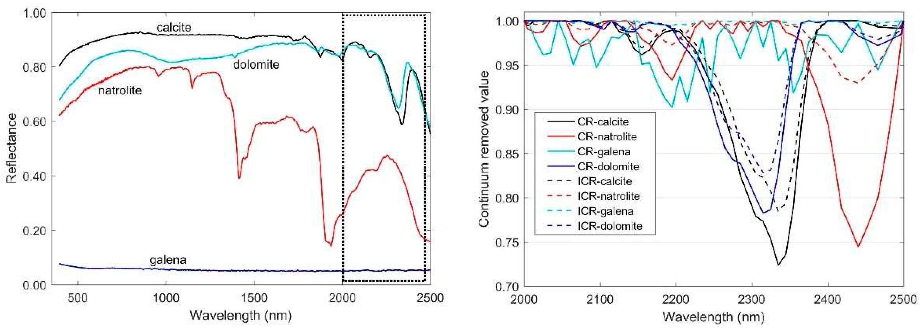
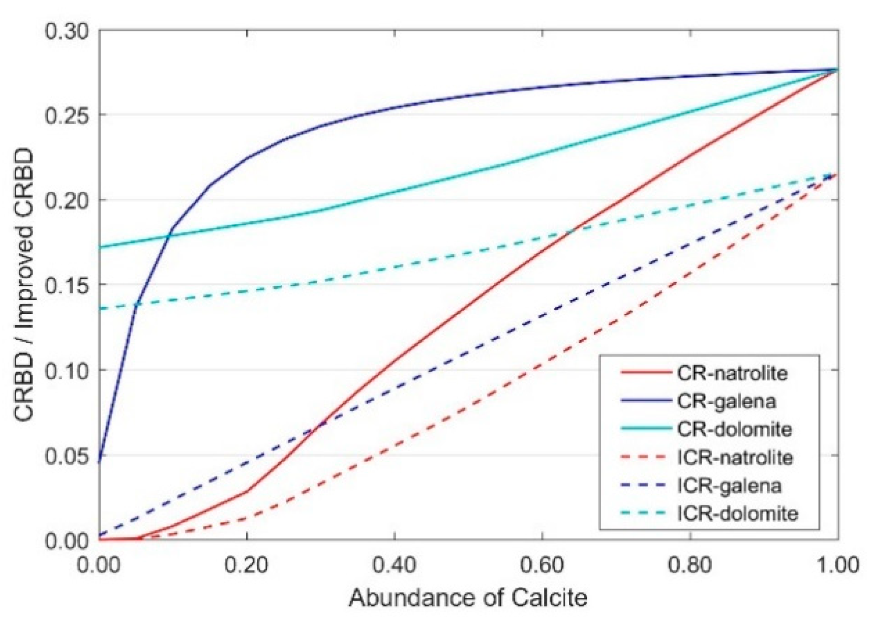
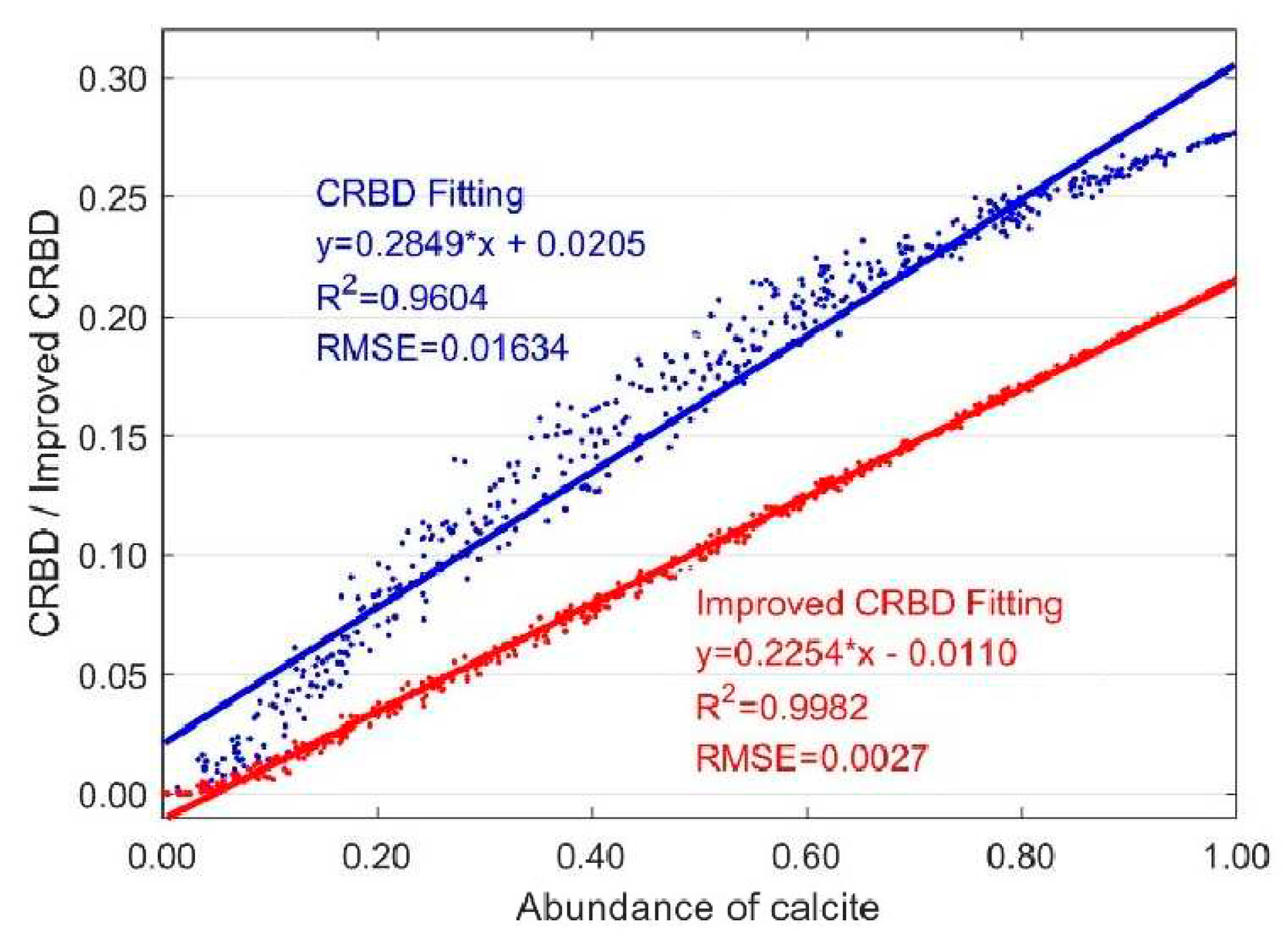
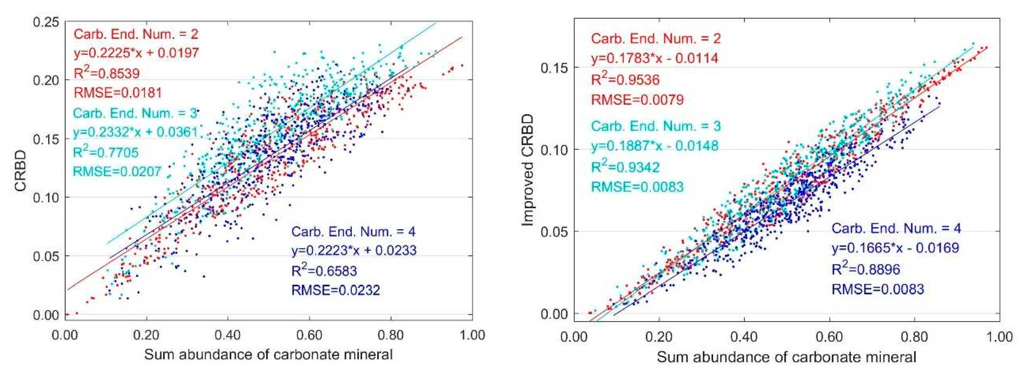
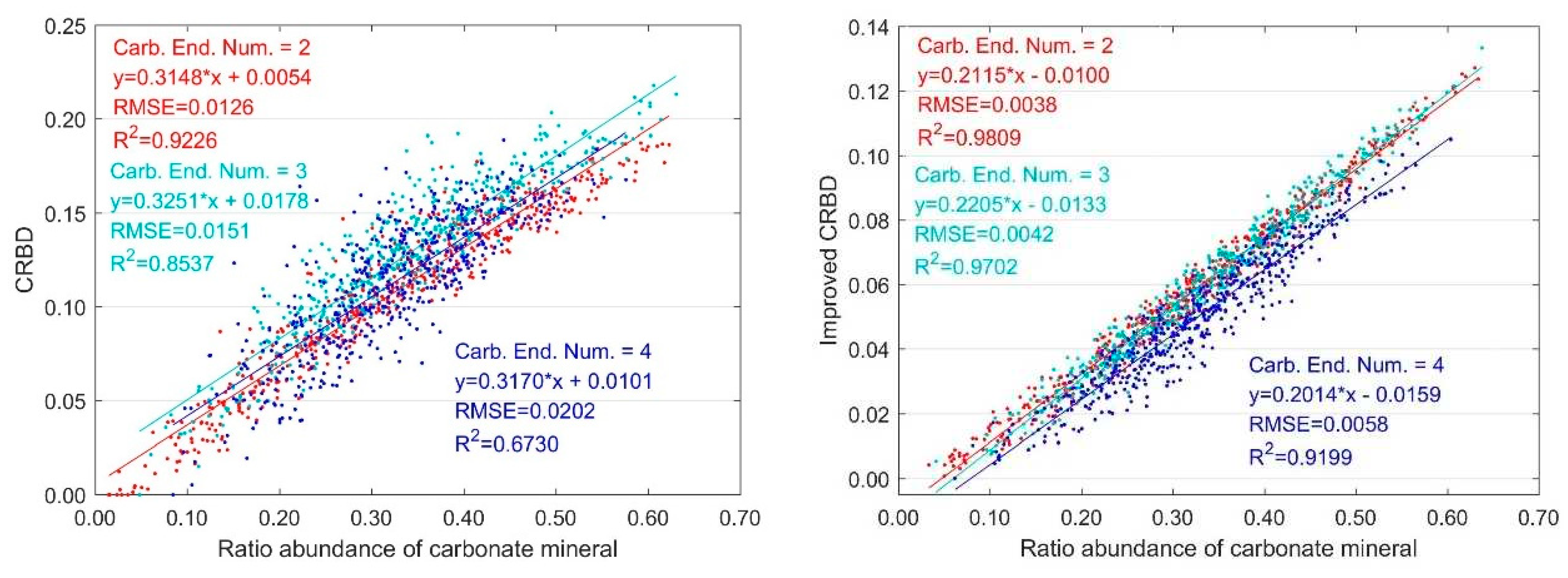
Carbonate Minerals Group1 (Absorption)	Other Minerals
Carbonate Minerals Group1 (Absorption)	Group 2 (Flat)	Group 3 (Reflected Peak)
Calcite(Ca[CO₃]) Dolomite ((Ca, Mg)[CO₃]2) Rhodochrosite (Mn[CO₃]) Strontianite (Sr[CO₃]) Witherite (Ba[CO₃]) Magnesite(Mg[CO₃])	Chalcopyrite (CuFeH₄S₂) Galena (PbS) Grossular (Ca₃Al₂[SiO₄]₃) Hematite (Fe₂O₃) Hypersthene ((Mg, Fe)[SiO₃]) Microcline (K[AlSi₃O₈]) Olivine((Mg, Fe)₂[SiO₄]) Quartz (SiO₂) Anorthite (Ca[Al₂Si₂O₈])	Heulandite (Ca[Al₂Si₇O₁₈]·6H₂O) Natrolite (Na₂[Al₂Si₃O₁₀]·2H₂O) Kaolinite(Al₄[Si4O10](OH)₈) Montmorillonite((Na,Ca)_0.33(Al,Mg)₂ [Si₄O₁₀](OH)₂·nH₂O ) Jarosite(KFe₃[SO₄]₂(OH)₆) Goethite (FeO(OH)) Buddingtonite ((NH₄)[AlSi₃O₈]) Hypersthene ((Mg,Fe)₂[Si₂O₆]) Chabazite((Ca, K₂, Na₂)₂ [Al₂Si₄O₁₂]₂·12H₂O)

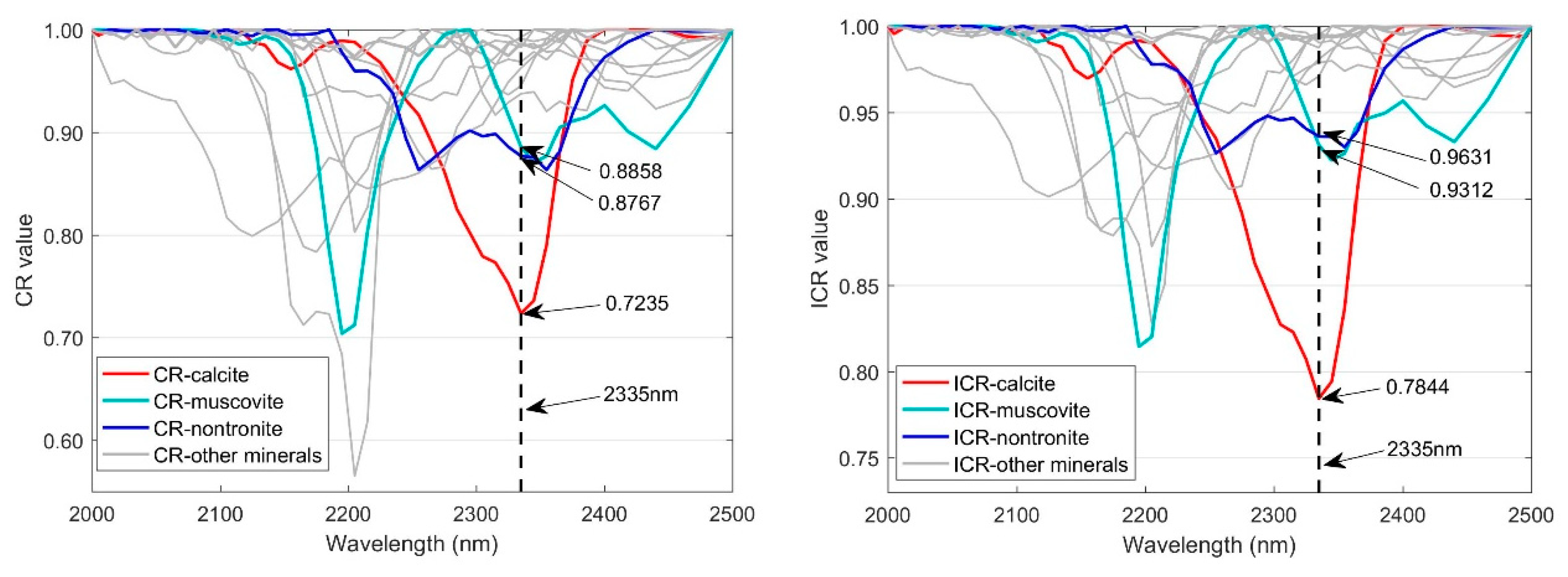
Table 2. Group classification for cuprite image data. The minerals marked by italic means the minerals are not carbonate but contain absorption at around 2.33µm.

Minerals with Absorption Group 1 (Absorption Valley)	Other Minerals
Minerals with Absorption Group 1 (Absorption Valley)	Group 2 (Flat Spectra)	Group 3 (Reflected Peak)
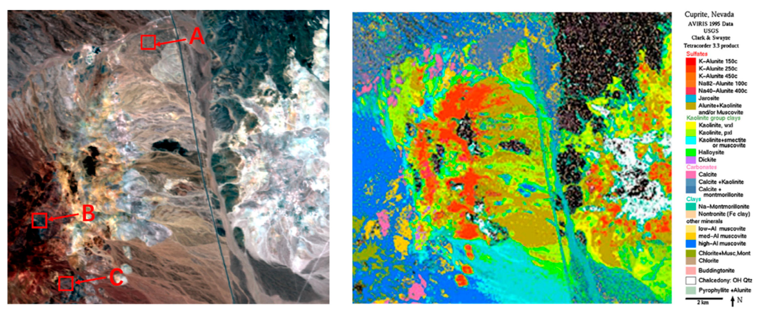
Calcite (Ca[CO₃]), Muscovite (KAl₂[AlSi₃O₁₀](OH)₂), Nontronite (Na_0.33Fe₂₃+(Al,Si)₄O₁₀(OH)₂·nH₂O)	Pyrope(Mg₃Al₂[SiO₄]₃), Dumortierite ((Al,Fe³⁺)₇BO₃[SiO₄]₃O₃), Sphene (CaTi[SiO₄](O,OH,Cl,F)), Desert varnish	Alunite (KAl(SO₄)₂·12H₂O), Buddingtonite ((NH₄)AlSi₃O₈·nH₂O), Kaolinite (Al₄[Si₄O₁₀](OH)₈), Jarosite (KFe₃[SO₄]₂(OH)₆), Chalcedony (SiO₂), Andradite (Ca₃Fe₂[SiO₄]₃), Montmorillonite ((Na,Ca)_0.33(Al,Mg)₂ [Si₄O₁₀](OH)₂·nH₂O )

Table 3. Evaluation by RMSE on carbonate mineral inversion by different methods.

Inversion Methods	Carbonate Endmember Number				Mean RMSE
Inversion Methods	1	2	3	4	Mean RMSE
Sum abundance with FCLS	0.0000	0.1682	0.1472	0.1487	0.1160
Ratio abundance with FCLS	0.0000	0.0598	0.0464	0.0923	0.0496
Sum abundance with MVCNMF	0.0825	0.2052	0.4177	0.4251	0.2826
Ratio abundance with MVCNMF	0.0389	0.1103	0.3207	0.1573	0.1568
Sum abundance with CMLNMF	0.0177	0.2264	0.2252	0.4800	0.2373
Ratio abundance with CMLNMF	0.0123	0.1433	0.2121	0.1712	0.1347
Sum abundance with GCICA	0.2116	0.3447	0.4395	0.2813	0.3193
Ratio abundance with GCICA	0.1758	0.2722	0.3568	0.1877	0.2481
Sum abundance with ACICA	0.1690	0.2552	0.3137	0.3953	0.2833
Ratio abundance with ACICA	0.1690	0.1848	0.2513	0.2108	0.2040
Sum abundance with CR	0.0639	0.1195	0.1365	0.1888	0.1272
Ratio abundance with CR	0.0639	0.0808	0.1006	0.1264	0.0929
Sum abundance with ICR	0.0348	0.0699	0.0727	0.1011	0.0696
Ratio abundance with ICR	0.0348	0.0379	0.0336	0.0536	0.0400

Table 4. Calcite abundance comparison between references and inversion results.

Algorithm	Calcite abundance
FCLS	0.1395
MVCNMF	0.1250
CMLNMF	0.3150
GCICA	0.1754
ACICA	0.2832
Inversion	0.2938(CR)	0.1268 (ICR)
RE	41.52%	38.92%

Table 5. The fitting results of different algorithms for Hyperion image.

Algorithm	Parameter of fitting equation		R2	RMSE
Algorithm	Slope	y-intercept	R2	RMSE
Calcite abundance with CR	0.2778	0.0440	0.9393	0.0099
Calcite abundance with ICR	0.1918	0.0135	0.9366	0.0070

Table 6. The retrieval abundance and RE value.

Inversion Method	Inverted Abundance		RE
Inversion Method	Position A	Position B	RE
FCLS	/	0.0747	-25.30%
MVCNMF	/	0.1334	33.40%
CMLNMF	/	0.1880	88.00%
GCICA	/	0.4119	311.90%
ACICA	/	0.1429	42.90%
CR	/	0.3314	231.40
ICR	/	0.1296	29.60%

Table 7. RMSE of inversion abundance by different simplified inversion equations.

Carbonate endmember number	Sum abundance with CR	Sum abundance with ICR	Ratio abundance with CR	Ratio abundance with ICR
1	0.1136	0.0410	0.1136	0.0410
2	0.3267	0.3152	0.2829	0.2558
3	0.4603	0.4494	0.3909	0.3684
4	0.5292	0.5454	0.36480	0.3605

Table 8. Carbonate minerals abundance comparison between references and inversion results.

Algorithm	Sum Abundance		Ratio Abundance
FCLS	0.2736		0.1885
MVCNMF	0.3993		0.2971
CMLNMF	0.2795		0.2565
GCICA	0.2222		0.1566
ACICA	0.2500		0.1762
Inversion	0.4719(CR)	0.2535 (ICR)	0.3463(CR)	0.1802(ICR)
RE	65.63%	-11.03%	61.08%	-16.18%

Table 9. The fitting results of different algorithms.

Algorithm	Parameter of Fitting Equation		R2	RMSE
Algorithm	Slope	y-Intercept	R2	RMSE
Sum abundance with CR	0.1634	0.0317	0.6097	0.0270
Sum abundance with ICR	0.1202	0.0019	0.7090	0.0157
Ratio abundance with CR	0.2657	0.0254	0.9226	0.0119
Ratio abundance with ICR	0.1861	0.0003	0.9731	0.0048

Table 10. RE of retrieval abundance from different algorithms.

Inversion method	RE		Mean RE
Inversion method	Position A	Position B	Mean RE
Sum abundance with FCLS	-8.83%	-24.76%	16.79%
Ratio abundance with FCLS	20.98%	21.77%	21.38%
Sum abundance with MVCNMF	-5.34%	-75.68%	21.45%
Ratio abundance with MVCNMF	41.53%	-55.96%	33.96%
Sum abundance with CMLNMF	-2.29%	-36.08%	19.18%
Ratio abundance with CMLNMF	-7.40%	32.46%	19.93%
Sum abundance with GCICA	-34.89%	8.02%	21.45%
Ratio abundance with GCICA	-55.59%	-12.33%	33.96%
Sum abundance with ACICA	-59.17%	-71.42%	65.30%
Ratio abundance with ACICA	-72.15%	-76.81%	74.48%
Sum abundance with CR	41.29%	-3.16%	22.22%
Ratio abundance with CR	111.77%	89.58%	100.67%
Sum abundance with ICR	-26.23%	-31.74%	28.98%
Ratio abundance with ICR	7.80%	-5.80%	6.80%

Disclaimer/Publisher’s Note: The statements, opinions and data contained in all publications are solely those of the individual author(s) and contributor(s) and not of MDPI and/or the editor(s). MDPI and/or the editor(s) disclaim responsibility for any injury to people or property resulting from any ideas, methods, instructions or products referred to in the content.

© 2023 by the authors. Licensee MDPI, Basel, Switzerland. This article is an open access article distributed under the terms and conditions of the Creative Commons Attribution (CC BY) license (http://creativecommons.org/licenses/by/4.0/).

Copyright: This open access article is published under a Creative Commons CC BY 4.0 license, which permit the free download, distribution, and reuse, provided that the author and preprint are cited in any reuse.

MDPI Initiatives

Important Links

Choose an area of interest and we will send you notifications of new preprints at your preferred frequency.

Disclaimer

Coupling Normalized Abundance with an Improved Continuum Removal Algorithm for Quantitative Inversion of Carbonate Minerals Using Hyperspectral Data

Abstract

1. Introduction

2. Data and Methods

2.1. Data

2.1.1. Spectra from the USGS Library

2.1.2. Synthetic Data

2.1.3. Hyperspectral Data

2.2. Methods

2.2.1. Linear Mixing Model

2.2.2. Construction of Improved Continuum Removal Algorithm

2.2.3. Abundance Normalization

2.2.4. Evaluation

3. CRBD/Improved CRBD Varies with Carbonate Abundance

3.1. Variation with One Carbonate Mineral

3.1.1. Variation with Two Endmembers Mixing

3.1.2. Variation with Multiple Endmember Mixing

3.2. Variation with Multiple Carbonate Minerals and Normalized Abundance

3.2.1. Variation with Sum Abundance

3.2.2. Variation with Ratio Abundance

4. Carbonate Mineral Abundance Inversion

4.1. Abundance Inversion of Synthetic Image Data

4.2. Abundance Inversion of Real Image Data, Cuprite Dataset

4.3. Abundance Inversion of Real Image Data, Hyperion Image Dataset

5. Discussions and Future Works

5.1. Simplified Abundance Inversion Model

5.1.1. Simplified Processing

5.1.2. Applications by Simplified Inversion Model

5.2. General Abundance Inversion Model

5.2.1. General Abundance Inversion Model by USGS Library

5.2.2. Abundance Inversion without Ground Samples

5.3. Considering the Absorption Influence of Non-Carbonate

5.3.1. Influence on Cuprite Image Data

5.3.2. Influence on Hyperion Image Data

5.4. Future Works

5.4.1. Relationship between Spectral Absorption and Carbonate Ion Concentration

5.4.2. Effects by Particle Size, Cation Types, and Other Factors

6. Conclusions

Funding

Data Availability Statement

Conflicts of Interest

References

MDPI Initiatives

Important Links

Subscribe