1. Introduction
Machine learning (ML) has become increasingly popular in data science applications due to its ability to analyze complex relationships automatically without explicit programming [
1]. Artificial neural networks (ANN), in particular, has gained attention for its capability to analyze large and complex datasets that cannot be easily simplified using traditional statistical techniques [
2,
3]. ANN has a long-established history in data science, and its wide range of applications makes it a powerful tool in data analysis, prediction and decision-making. ANNs can detect non-linear relationships between input variables, extending their application to various fields like healthcare, climate and weather, stock markets, transportation systems and more. ANNs has also proved its applicability in handling problems in agriculture, medical science, education, finance, cyber security, and trading commodity. These neural networks have successfully found solutions to problems that could not be solved by the computational ability of conventional procedures. ANN has been keenly used by researchers in the field of water resources management such as estimation of evaporation losses, exploration of association between groundwater and drought, the prediction of groundwater salinity, groundwater quality forecasting, prediction of suspended sediment levels, determination of flow friction factors in irrigation pipes, rainfall-runoff estimation, studying soil moisture using satellite data, modeling of contaminant transport, mapping vulnerability of saltwater intrusion, and modeling of irrigation water infiltration [
4,
5,
6,
7,
8,
9,
10,
11,
12,
13,
14,
15]. The applications of artificial intelligence in predicting and monitoring groundwater quality and quantity are rapidly growing. ANN offers advantages in reducing the time needed for data sampling and its ability to identify the nonlinear patterns of input and output makes it superior compared to other classical statistical methods. These prediction models have the potential to be very accurate in predicting water quality parameters [
16,
17,
18,
19]. In the recent times, ANN, ANFIS and fuzzy logic are being widely used in predicting and monitoring groundwater quality and quantity [
20,
21,
22]. Nonlinear methods such as ANNs, which are suited for complex models, are used for the analysis of real world temporal data. Neural networks provide a powerful inference engine for regression analysis, which stems from its ability to map nonlinear relationships, which is more difficult and less successful while using conventional time-series analysis [
23].Since environmental data is inherently complex with data sets containing nonlinearities; temporal, spatial, and seasonal trends; and non-gaussian distributions, neural networks are widely preferred [
9,
24,
25,
26].
One of the main advantages of ML is that, it helps in solving scaling issues from a data-driven perspective and can also help to build uniform parameterization schemes. The new advances in ML models present new openings to understand the network instead of perceiving it as a black box. These models can be combined with other algorithms for optimization to yield better results and robust models. Researchers combined the ability of nature-inspired optimization algorithm to optimize the neural networks and help producing better prediction results. Ref. Lu et al.[
27] adopted ant colony optimization (ACO) model to train the perceptron and to predict the pollutant levels. The approach was proved to be feasible and effective in solving real air quality problems and by comparing with the simple back propagation (BP) algorithm [
27]. A modified ACO in conjugation with simulated annealing technique was aslo studied [
28]. ACO-based neural network was used for the analysis of outcomes of construction claims and found that the performance of ACO-based ANN is better than BP [
29].
Groundwater plays a significant role in satisfying global water demand. Globally, over 2 billion people rely on groundwater as a primary source of water [
30]. Several regions of the world depend on the use of groundwater for various requirements. In India too, about 80% of the rural population and 50% of the urban population uses groundwater for domestic purposes [
31]. Overexploitation in several parts of the country has resulted in groundwater contamination, declining groundwater levels, drying of springs and shallow aquifers, and land subsidence in some cases [
16,
32,
33]. Along with declining water levels, deterioration of groundwater quality has also become a growing concern. Groundwater quality depends on geological as well as the anthropogenic features of a region. Over the past decades, many anthropogenic and geogenic contaminants in groundwater have emerged as serious threats to human health when consumed orally. Ingestion of contaminated groundwater can cause severe health effects and can also cause chronic health conditions like cancer [
34,
35]. Thus, groundwater quality assessment and monitoring are necessary considering the potential risk of groundwater contamination and its effects on suitability for human consumption [
36,
37,
38,
39]. Hence, water quality monitoring plays an important role in water resources management. Conventional water quality monitoring techniques involve manual collection of water samples and analysis in the laboratory. This process is expensive, time consuming and involves lot of manual labor. Data-driven models based on artificial intelligence can efficiently be used to solve such problems and overcome these difficulties especially when historic quality data is available. The conjunction of ACO with ANN is a technique used successfully in optimizing parameters in other research areas. However, until now no one has explored the applicability of this technique to predict multiple groundwater quality parameters, although it has been used in several other domains in water resources management. Hence, the aim of our study is to build an ant colony optimized multiperceptron neural network for predicting multiple groundwater quality parameters.
2. Methodology
2.1. Multilayer Perceptron Neural Network (MLP-NN)
An MLP is a type of neural network that is widely used for forecasting applications. It comes under the category of feedforward algorithms, since inputs are combined with the initial weights in a weighted sum and subjected to the activation function [
40]. In an MLP-NN, each linear combination of data is propagated to the next layer through a perceptron and multiple layers of interconnected neurons process the input data to produce the output data. Backpropagation algorithms are used in MLPs, to adjust the weights between the neurons and improve the accuracy of the network’s predictions [
41]. In MLPs, generally unknown connection weights are adjusted to obtain the best match between a historical set of model inputs and the corresponding outputs. The construction of a neural network model involves three steps. i) Training stage is the priliminary step, in which the network is exposed to a training set pertaining to the input–output patterns. ii) Testing stage is the second step in which the network’s performance is evaluated. Consequently, the third step is the validation stage, in which the network’s performance is evaluated. The expression for an output of an MLP is given by equation 1.
In the equation, W
tj is a weight in the output layer connecting the j
th neuron in the hidden layer and the k
th neuron in the output layer, W
ji is the weight of the hidden layer connecting the i
th neuron in the input layer and the j
th neuron in the hidden layer, W
j0 is the bias for the j
th hidden neuron, f
h is the activation function of the hidden neuron, W
t0 is the bias for the kth output neuron, ‘f’ is the activation function for the output neuron, X
i is i
th input variable for input layer and y
t is computed output variable, N
n and M
n are the number of the neurons in the input and hidden layers. Neurons in each layer are linked to neurons in the next layer with varying weights, and each neuron in a layer receives input signals from the previous layer’s neurons, which are multiplied by the corresponding connection weights. The model has been trained with appropriate number of epochs to reduce the error and improve the learning rate of the model. One of the callbacks, Early Stopping has been used, so that the model will terminate itself when the monitored quantity has finished improving based on the weights. The backpropagation procedure decides the error value by computing the distinction between the predicted value and expected value, beginning from an output layer towards the input layer. It is indicated by the symbol
, which is equivalent to the error of node i in layer l.
This is a repetitive process, and after modifications of the weights, the procedure is simulated again until convergence of output.
2.2. ACO
Ant Colony Optimization (ACO) is a metaheuristic optimization algorithm inspired by the behavior of ants searching for food [
42]. ACO is used to find optimal solutions to complex optimization problems [
43]. The algorithm involves a set of artificial ants that search for a solution by iteratively constructing candidate solutions and evaluating their quality using a heuristic function and a pheromone trail. The pheromone trail represents the cumulative experience of the ants in finding good solutions, and ants are more likely to select components with a higher pheromone level. Over time, the pheromone trail is updated to reflect the quality of the solutions found by the ants. ACO has been applied to a wide range of optimization problems and has the ability to handle complex, non-linear, and non-differentiable objective functions. It has been successfully applied to optimizing weights in ANNs [
44,
45,
46]. In
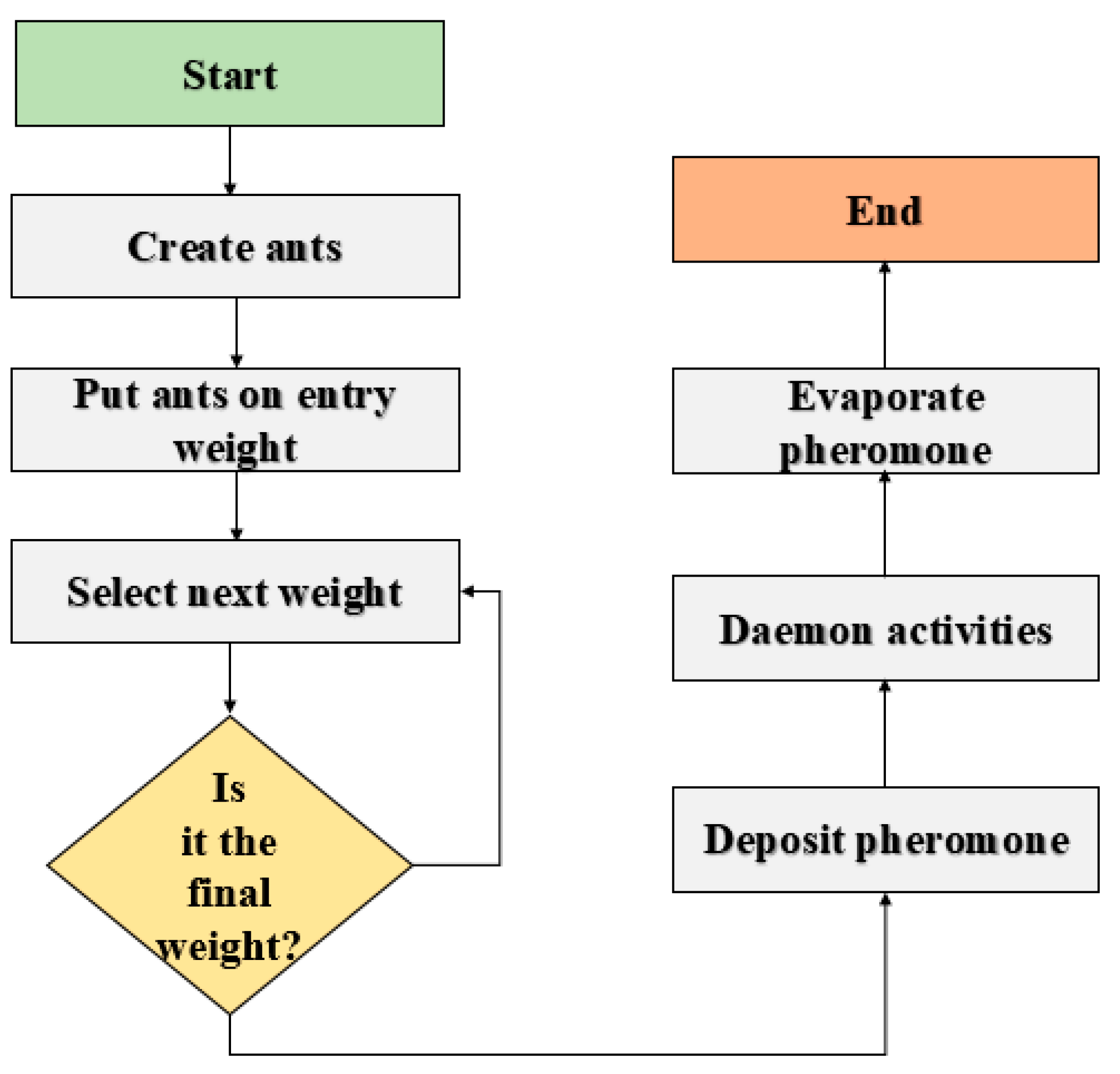
Figure 1, the general ACO algorithm for optimizing weight is illustrated. The framework of ACO is split into three components. The first component involves the initialization of the pheromone trail. The second component involves each ant building a solution to the problem using a probabilistic condition transition rule, which is subjected to the condition of the pheromone. The third component is updating of the quantity of pheromone according to rules set. The first phase is the evaporating of a part of the pheromone and the second phase is the addition of pheromones of each ant. This process is proportional to the fitness of its solution. This step is iterated until the stopping criterion is achieved.
2.3. MLPNN and ACO
In MLPNN, training the model is one of the most important steps. The ability of ants to search for optimal food paths is combined with neural networks in order to optimize the weights and biases of the network. [
47,
48,
49].The algorithm works by simulating the behavior of ants as they search for food. In this case, the “food” represents the optimal set of weights and biases that minimize the network’s error. The ants in the ACO algorithm search for the optimal set of weights and biases by depositing pheromones on the connections between neurons in the network. The strength of the pheromones is proportional to the fitness of the solution represented by that connection. Ants then use these pheromone trails to guide their search for better solutions. As the ants continue to search, the pheromone trails are updated based on the quality of the solutions found. This process allows the algorithm to converge towards the optimal solution over time. The step-by-step procedure of building an ACO-MLPNN is described below.
Step 1. Initialize the parameters of ACO and ANN, including the weights and biases of the ANN
Step 2. Initialize a population of ants
Step 3. Evaluate the fitness of each ant using the ANN and the current weights
Step 4. Update the pheromone levels on the paths based on the fitness of the ants
Step 5. Choose the best ant as the global best solution
Step 6. Use the global best solution to update the weights and biases of the ANN
Step 7. Repeat steps 2-6 until a stopping condition is met
Step 8. Return the best solution found
ACO has several advantages for MLPNN weight optimization. First, it is a population-based algorithm that has the ability to search a large weight space efficiently. Second, it can handle non-convex and multimodal fitness landscapes, which can be challenging for other optimization algorithms. Third, it can find good solutions even when the weight space has many local optima, which can be difficult to escape for other optimization algorithms.In in a hydrological study, the temporal and spatial variation of parameters play a greater role. Inorder to consider the interplay betwen the parameters, and the time, the algorithm was constructed, and site-specific models were developed. Though the base is equation 1, site specific models developed were different and based on the time-series of multivariate dataset. Hence, we have combined the davnatges od ANN and ACO with
Is it not necessary to talk about time series? Multi parameter? Multi criteria
2.4. Data Acquisition and Processing
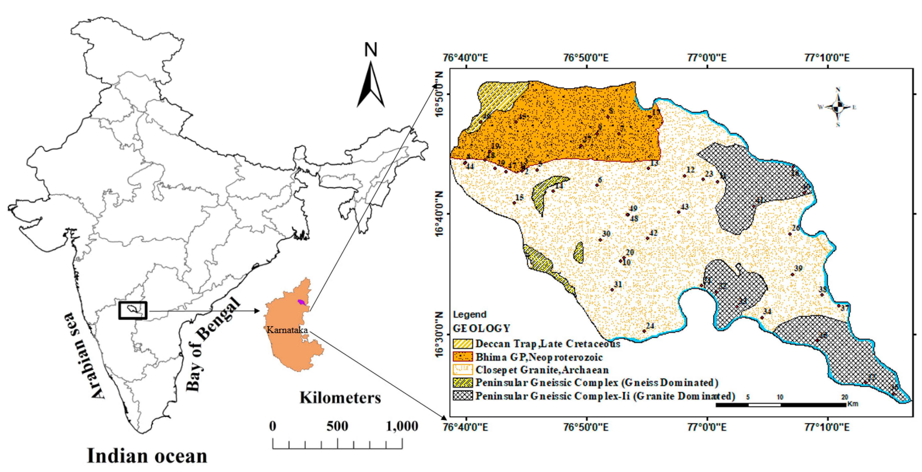
In order to study the efficiency of this model, a real dataset of a study area located in the Yadgir district of Karnataka, India (
Figure 2). Groundwater samples were collected from 50 wells periodically from the year 2014 to 2020 [
50,
51]. The samples were collected in 250-ml polyethylene bottles that were pre-washed with a 1:1 diluted HNO
3 solution and rinsed with in the water to be sampled before each sampling event. In the field, parameters such as, pH, HCO
3 and EC, were analyzed and Ca
2+, Mg
2+, Na
+, K
+ , U
2+ and Cl
− were measured in the laboratory following the standard procedures as explained in [
51]. The ion balance error was calculated for analytical precision, which was within ± 10%.
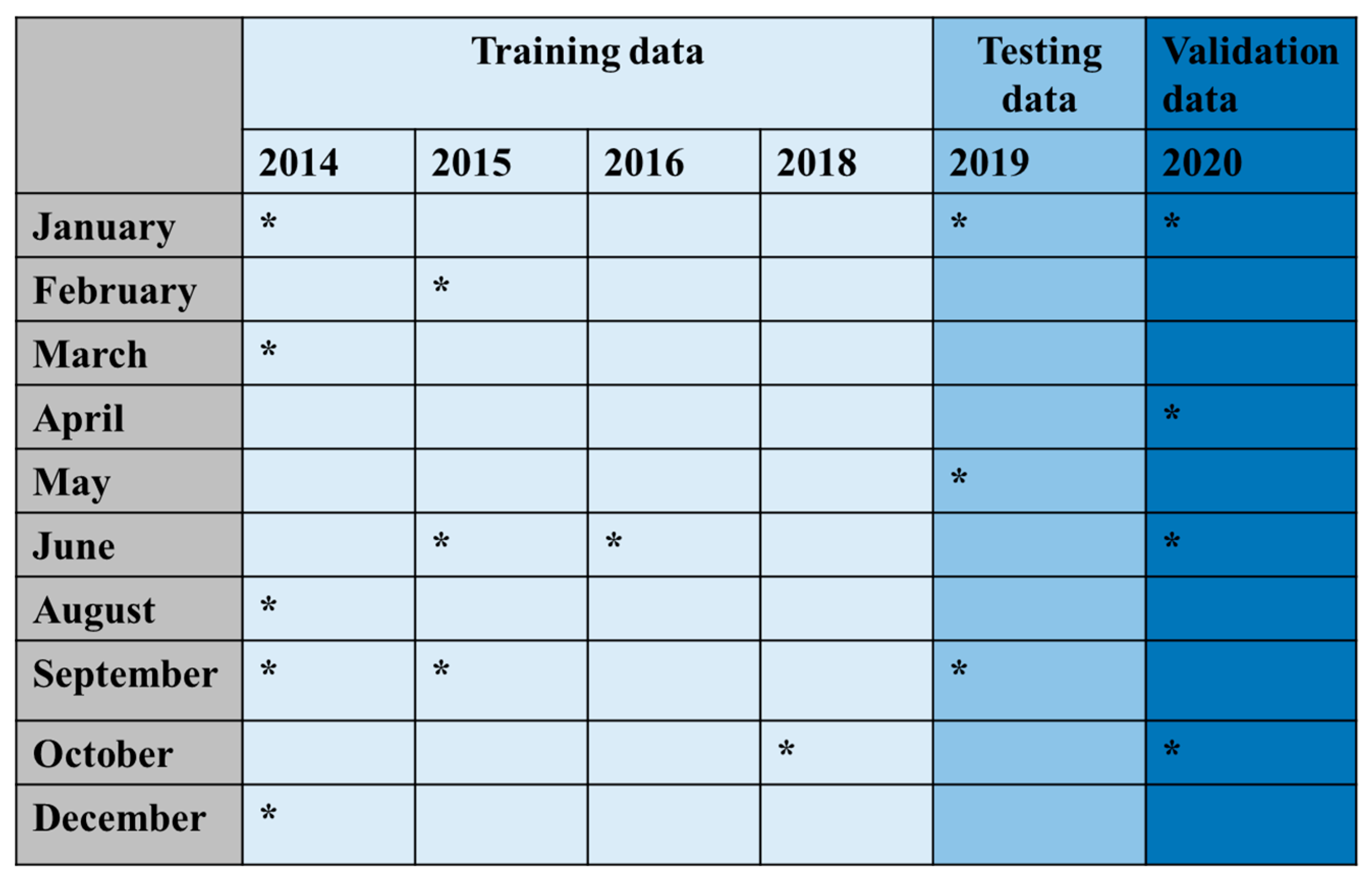
The collected quality parameters were saved in a csv file, and were split as training data, testing data and validation data. Convenience sampling was used to split the data for training, testing and validation since it is a time series dataset [
52]. 80% of the data was used for training, and the remaining 20% for testing and validating.
Table 1 describes the sample collection period and the distribution of training, testing and validation data.
2.5. Model Performance Evaluation
Performance evaluation of the trained artificial neural network model was carried out to have an understanding of how good the developed model was. To evaluate the performance and error of the artificial neural network model was measured with three different metrics such as, i) coefficient of multiple determination (R2), ii) the root mean squared error (RMSE) and iii) Nash–Sutcliffe efficiencies (NSE) given by Equations (3), (4), (5) and (6), respectively.
Coefficient of Determination
The Coefficient of Determination, denoted as R², is a statistical measure that evaluates how well a linear regression model fits the data [
41]. It is a value between 0 and 1 that represents the proportion of the variation in the dependent variable that is explained by the independent variable in the model. R² is calculated by taking the ratio of the sum of squares of the regression (SSR) to the total sum of squares (SST).
Root Mean Squared Error (RMSE)
The root-mean-square error (RMSE) measures the difference between the actual values of the dependent variable and the predicted values of the dependent variable produced by the regression model. RMSE is commonly used in various applications such as in finance, engineering, and environmental studies to evaluate the accuracy of models used for forecasting and prediction. It is a measure of the average magnitude of the errors between the predicted and actual values of the dependent variable. A lower value of RMSE indicates that the model has a better fit to the data and is more accurate in its predictions.
Nash–Sutcliffe Efficiencies (NSE)
NSE is a commonly used statistical measure to evaluate the performance of hydrological or environmental models. It is a measure of how well the simulated values from a model match the observed values, and it is based on the ratio of the residual sum of squares (RSS) to the total sum of squares (TSS) of the observed data. In Equation (5), RSS is the residual sum of squares, which is the sum of the squared differences between the observed and simulated values, and TSS is the total sum of squares, which is the sum of the squared differences between the observed and mean observed values.
Mean absolute Error (MAE)
MAE is a measure of the average magnitude of errors in a set of predictions or estimates. It is used to evaluate the accuracy of prediction models by measuring the difference between predicted values and actual values. MAE is calculated by taking the absolute difference between the predicted and actual values and then taking the average of those differences. The formula for MAE is:
3. Results and Discussions
3.1. Statistical Description of Data
The descriptive statistics of groundwater quality parameters were computed and given in
Table 2. The mean value of EC is 2227.78 μS/cm, Ca is 87.39 mg/l, Na is 270.7 mg/l. K is 7.31 mg/l, Mg is 57.43 mg/l, F is 1.20 mg/l, Cl is 400.79 mg/l, U is 26.28 mg/l and HCO3 is 411.76 mg/l. Interpreting the skewness values, it is observed that all selected parameters were positively skewed and ranged between 0.87 to 4.18. This indicated that indicated that their distributions have longer right tails and are concentrated towards the left. In general, a kurtosis value greater than 3 indicates a distribution that is more peaked and has heavier tails than a normal distribution, while a value less than 3 indicates a flatter distribution with lighter tails (Westfall 1905). The kurtosis value for pH (4.81), K (7.62) and F (7.44) is positive, and indicates that the distribution is more peaked than a normal distribution. This means that there are more extreme values in the dataset than would be expected for a normal distribution. The kurtosis value for EC (12.26), Ca (12.64), Mg (13.82), Cl (18.71), U (17.71) and Na (15.43) is positive, and indicates that the distribution is highly peaked and has more extreme values than a normal distribution. The kurtosis value for HCO
3 is very close to zero (0.05), which indicates that the distribution is roughly similar in peakedness to a normal distribution.
3.2. ACO-MLPNN Model Formulation
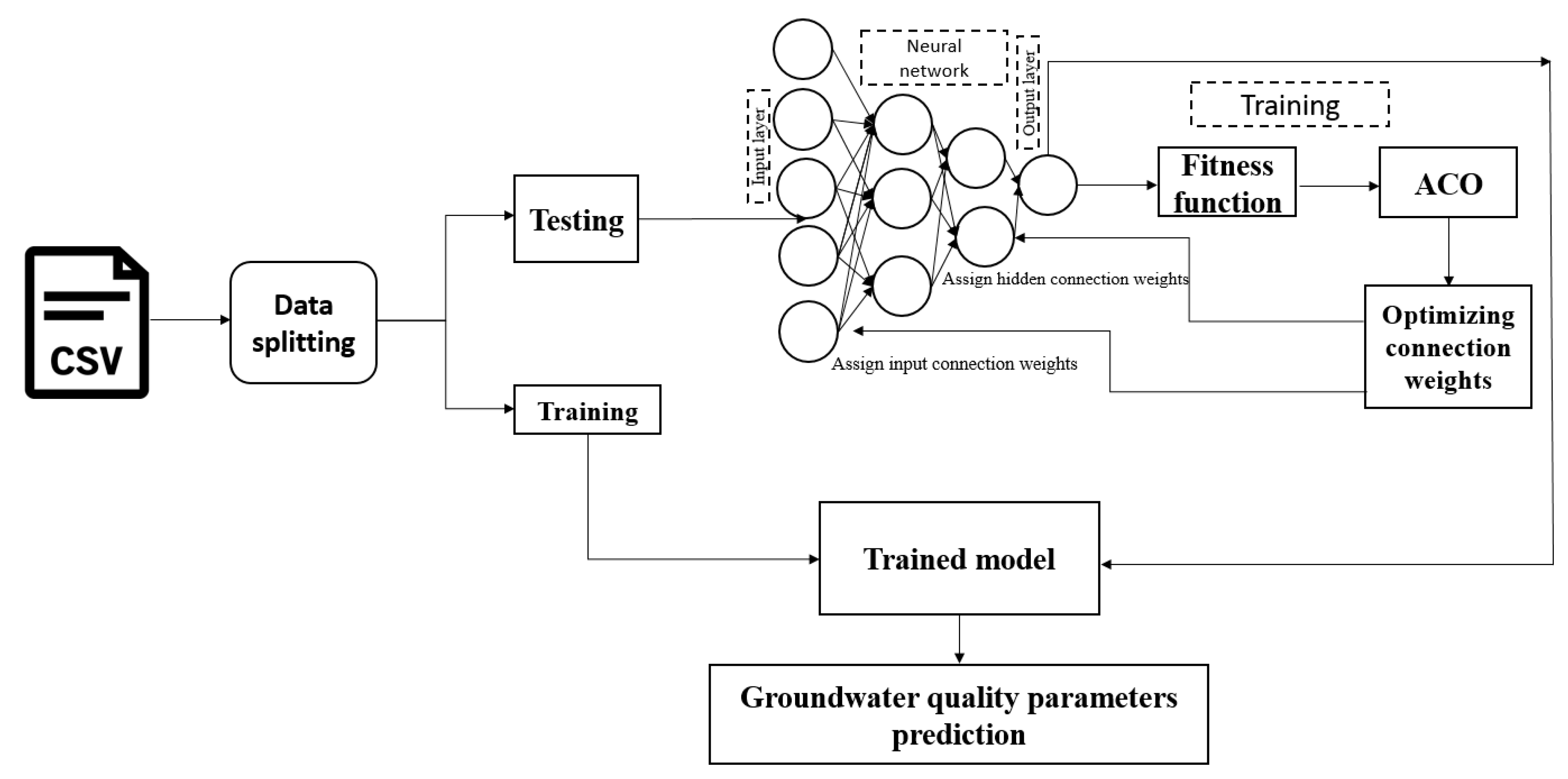
In construction of an ANN model, training is the first step. The model is introduced to the input–output patterns. Each layer contains nodes that have distinct classifications according to their locations. Nodes at the first layer are introduced as the input data. The second layer, which is also known as the hidden section of model and constitutes the hidden layers, (neurons); and mathematical calculations are used to find relationships between parameters. Finally, the output of this system is provided at the third layer. The connection between inputs, hidden and output layers consist of weights and biases that are considered parameters of the neural network. ACO has several advantages for MLPNN weight optimization. The weighted output is then passed through a transfer function. After trial and error, the hidden neurons were set to 6. After initializing the network weights and biases during the training process, iterative adjustments of the weights and biases pertaining to the network were carried out. We have predicted 10 different parameters, and the model for each parameter and each well location is independent and does not have any connection with the models of other parameters and locations developed. Hence, we have 10 separate models for each parameter considered.The most popular algorithm for training neural networks is the back-propagation method. Backpropagation is a first-order optimization method based on the steepest descent algorithm that requires a learning rate to be specified. In this study, we use the default training function ‘trainlm’ for training the hybrid model: ‘trainlm’ is the Levenberg–Marquardt back-propagation training algorithm, which updates the weight and bias values according to the Levenberg–Marquardt procedure. In ACO, the weights of an ANN are represented as pheromone values, and ants, mimicking the foraging behavior of real ants, select weights based on these pheromone values and heuristics. The ants then update the pheromone values based on the quality of the solution found, and pheromone evaporation is applied to encourage exploration and prevent stagnation. This process is repeated for a certain number of iterations, and the best solution found by the ants, which corresponds to the set of weights resulting in the lowest error, is selected as the final solution for the ANN. However, due to the stochastic nature of ACO, careful tuning of parameters and multiple runs may be necessary to achieve optimal results. ACO can be a promising approach for optimizing ANN weights, but it requires careful experimentation and parameter tuning to achieve the best performance. While selecting the best fitting MLPNN, the number of neurons was set to be 20 with the constant learning rate and momentum of 0.1 and 0.9, respectively. The workflow sequence of the ACO-MLPNN is shown in
Figure 3.
3.2.1. Predicting temporal variation
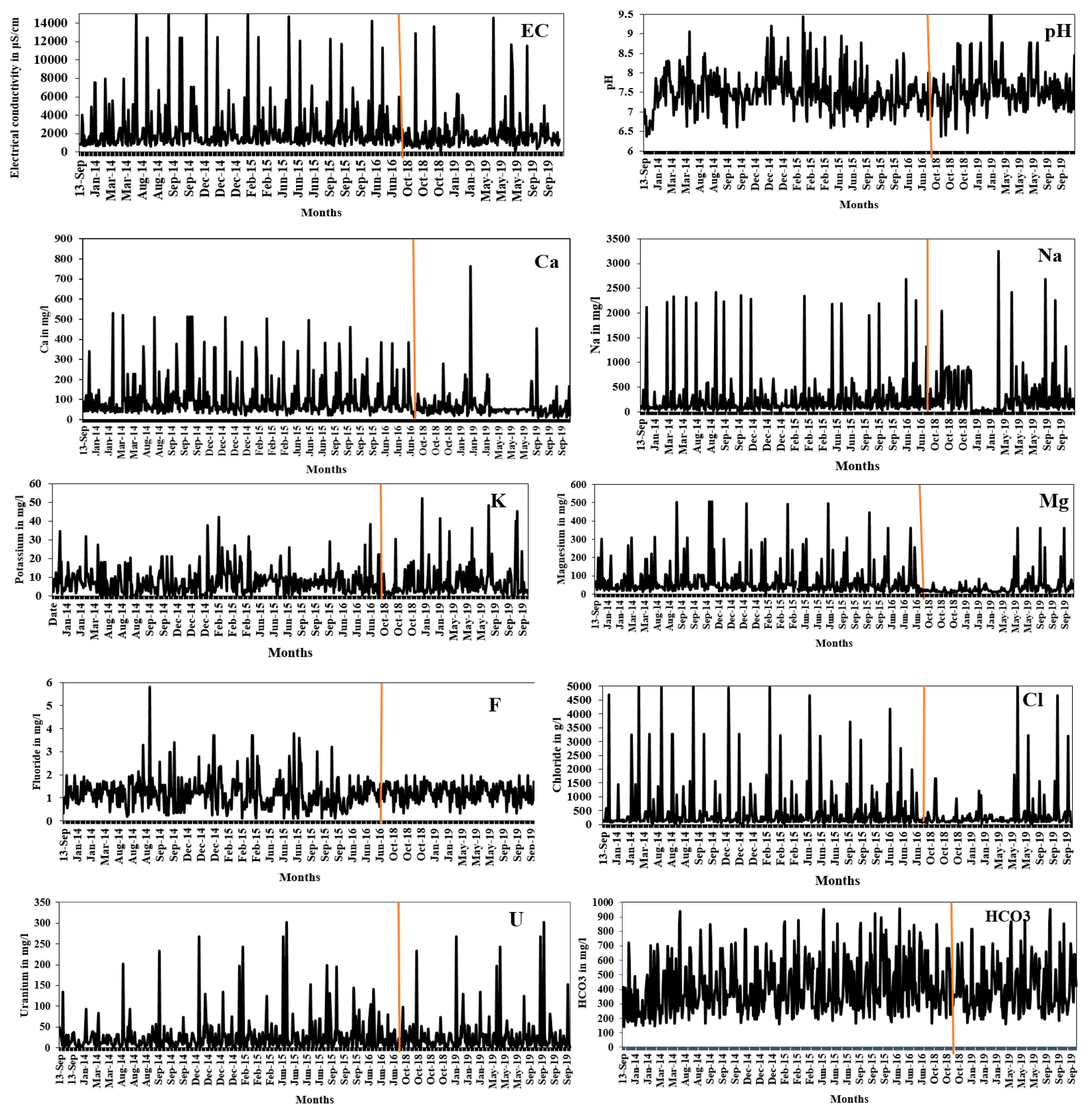
In the constructed ACO-MLPNN network, data from 2014, 2015 and 2016 are used for training. Data from 2018 and 2019 are used to testing and 2020 data is used for validation.
Figure 4 represents the temporal variation of all the parameters considered for training and testing of the neural network.
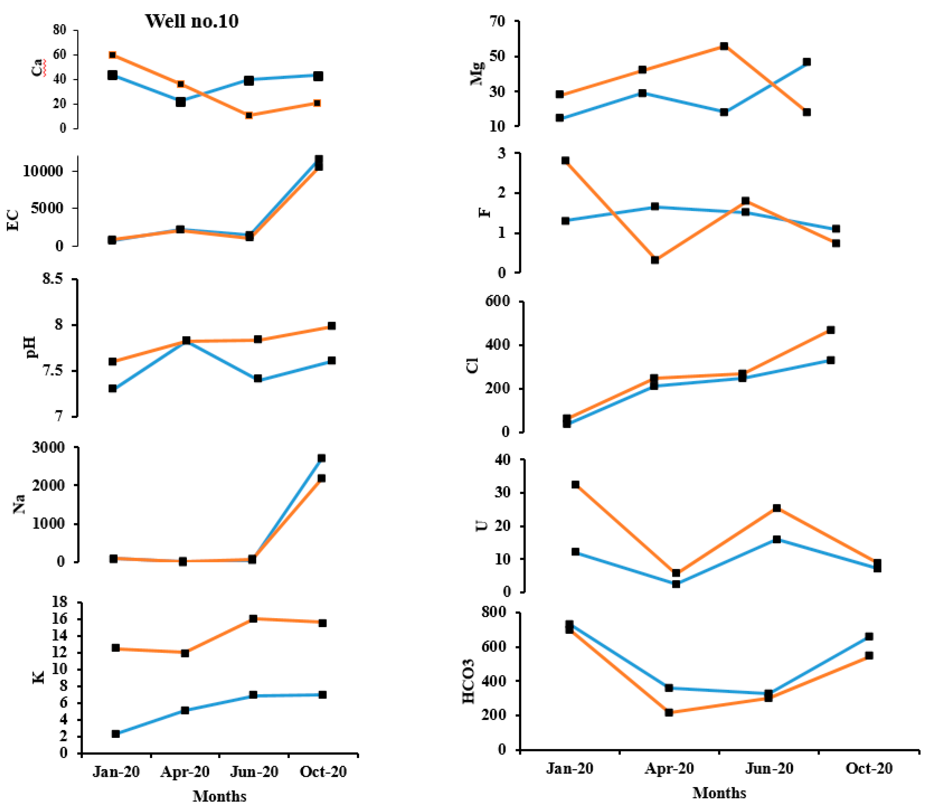
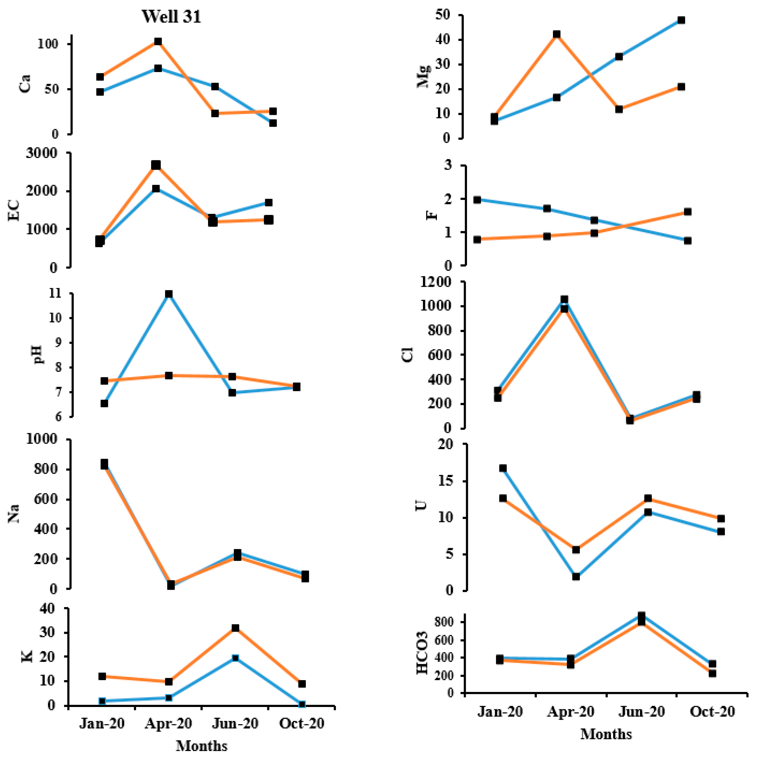
The temporal observed and predicted data for the validation data set for January 2020, April 2020, June 2020 and October 2020 appears to be in reasonable acceptance with each other. As an example, the observed and predicted quality parameters of well no. 10 and well no.31 are shown in
Figure 5 and
Figure 6 respectively. In well no. 10, except for F
-, all other ions have a good prediction. In well no. 31, except pH and F
-, all other ions have a good prediction. This may be attributed to the fact that pH and F
- have considerably less variance and standard deviation as compared to the other parameters. Also, when the range of values is within a small limit, the prediction appears to be poor.
In order to study the temporal variation of predicted parameters in a closer scale, well no.10 and well no 31 were chosen (
Figure 5 and
Figure 6). It can be inferred that the prediction of F
- and pH has great variation from the observed concentration. As discussed, this could be attributed to the range of parameter concentration and the variance. The ability of ACO-MLPNN to predict other parameters such as HCO
3 and EC, were analyzed and Ca
2+, Mg
2+, Na
+, K
+, U
2+ and Cl
− have been reasonably good.
3.2.2. Predicting Spatial Variation
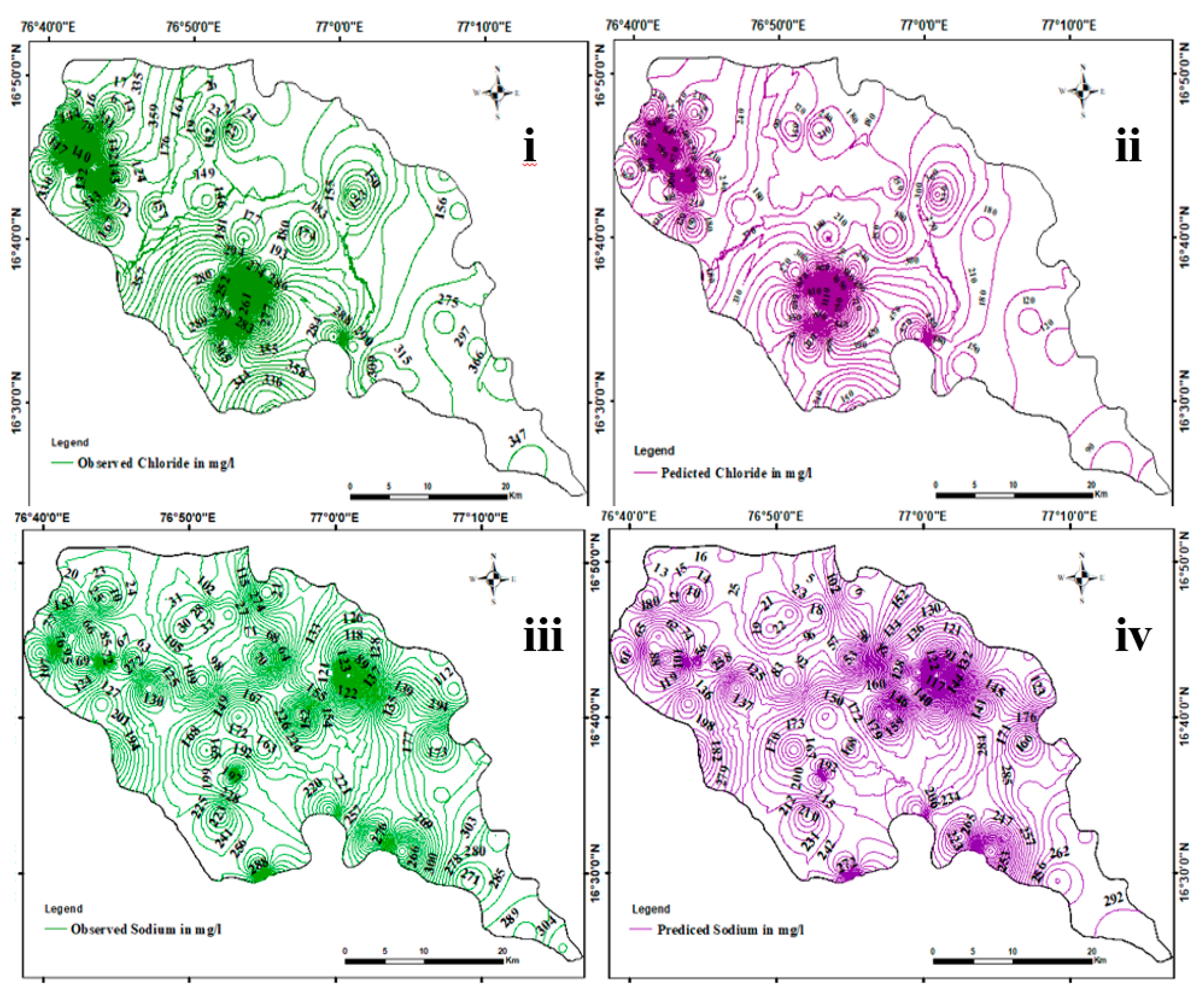
The spatial variability of the predicted concentration of parameters were studied. The spatial distribution of the observed and predicted data for Na
+ and Cl
- for January 2020 are shown in
Figure 7. The results are based on the past data, and each prediction is a separate model and also, there is not connection between any well. Although, the index variable for training the network is the “location of the well”, all the wells lie within the same regions and the groundwater networks could be interconnected. The network constructed by us does not consider that geological complexity, and hence that could be a drawback.
3.4. Performance Measures for ACO-MLPNN model
To quantify the error between the observed and predicted values, various performance efficiency parameters were used. R
2, RMSE, NSE and MAE (equations 3,4,5 and 6) are the efficiency parameters that were chosen (
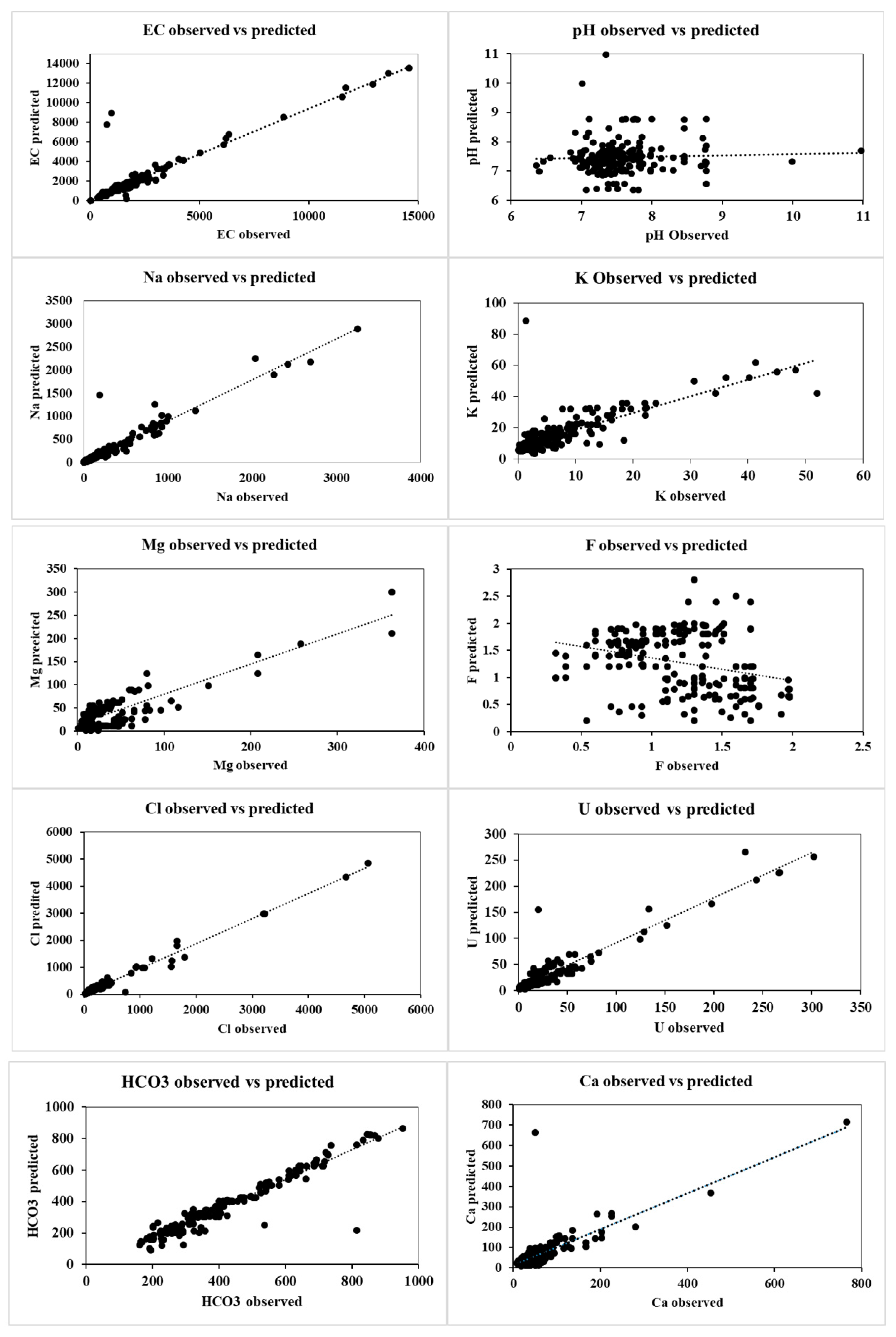
Table 3). The utilization of four statistical indices to evaluate the performance of the proposed model offers several advantages. Firstly, it ensures that the maximum error obtained during the evaluation process is within an acceptable range for a forecasting model. A linear correlation between the observed and predicted parameters are shown in
Figure 8. Except for pH, and F
-, all the other parameters appear to be in good acceptance with the observed values.
The use of RMSE allows for a check on the sum of errors over the validation period, ensuring that it is not too high. Furthermore, the use of other indices provides a consistent level of errors, which is important in ensuring that the model’s performance is reliable when applied to unseen data in the testing period. Using multiple indices provides a more comprehensive evaluation of the model’s performance. Each index captures a different aspect of the model’s accuracy, and together they can give a more complete picture of the model’s strengths and weaknesses. In this way, the combined use of both R2, RMSE, NSE and MAE indices provides a great potential for maintaining a consistent level of error throughout the model evaluation process. The
These statistical indices represent the performance of the built ACO-MLPNN model for predicting various water quality parameters. Based on the given indices, the ACO-MLPNN model performed well for some parameters such as NSE for pH, Cl, and HCO3, and R2 for Na and U. However, the model performance was not satisfactory for some parameters, such as NSE for EC, Na, and K, and RMSE for EC and Na. For pH the R2 value is 0.04. This indicates that the model’s ability to predict the variance in pH values is low, the RMSE value is 0.70, which indicates that the model’s average prediction error for pH is moderate for pH is 0.99, indicating that the model’s predictions for pH are very close to the observed values, with only a small difference. Whereas, the MAE for pH is 0.53 indicating that the model’s predictions for pH is mostly accurate, with relatively low error. Similarly based on the results, the model seems to perform well for some parameters such as Na+, Cl-, HCO3-, and U2+ with relatively high R2 values and low RMSE and MAE values. However, the model performs poorly for some parameters such as EC, Ca2+, K-, and Mg2+ with low R2 values and high RMSE and MAE values. In some cases, the NSE value is negative, indicating that the model performs lower than the mean value.
4. Conclusion
Machine learning models are being extensively used for classification, regression and prediction across different industries and applications. In the field of hydrogeology, they provide valuable insights into groundwater quality, allowing for effective management and protection of this critical resource. In order to study the efficiency of machine learning, an ant colony optimized multilayer perceptron neural network was used on a real groundwater quality dataset collected from northern Karnataka, India. This technique was used to predict pH, EC, Na+, Ca+, Na+, K+, Mg2+, F-, Cl- and U+ from 50 selected wells in this region. The temporal variation of the predicted groundwater quality was compared with the observed quality parameters. The model for each well location and each parameter is unique.Performance efficiency was checked using R2, RMSE, NSE and MAE pefomance metrics. This model gave reasonable prediction accuracy for parameters whose standard deviation was high.However, for parameters with a smaller range did not show great prediction results. The network suggested by us utilizes the ACO algorithm for optimizing ANN weights, but it requires careful experimentation and parameter tuning to achieve the best performance. The spatial prediction also shows considerable correlation with the observed values. However, this cannot replace sampling and analysis, and this will certainly help in reducing the temporal frequency of sample collection. Another major advantage is that, we can constantly keep adding data as and when field data is available, and this will improve the model performance further. This technique can also be used in other domains which deal with multi-variant, spatial and temporal datasets.The ACO-MLPNN model may need further optimization and calibration to improve its performance for some parameters, however, it predicts good results for other parameters. Hence, the ACO-MLPNN model developed by us can be considered as a robust tool to predict groundwater quality parameters. This study will help in forecasting the status of groundwater quality in a region and can save from quality detorioration.
Acknowledgments
The authors would like to thank Dr. Manoj Subramanian and Dr. Thirumurugan for conducting sample collection and laboratory analysis from 2014-2016.
References
- Frank, M.R., Wang, D., Cebrian, M. et al. The evolution of citation graphs in artificial intelligence research. Nat Mach Intell 1, 79–85 (2019). [CrossRef]
- Oludare Isaac Abiodun, Aman Jantan, Abiodun Esther Omolara, Kemi Victoria Dada, Nachaat AbdElatif Mohamed, Humaira Arshad,State-of-the-art in artificial neural network applications: A survey,Heliyon,Volume 4, Issue 11,2018,e00938,ISSN 2405-8440. [CrossRef]
- Wang, H. He and D. Liu, “Intelligent Optimal Control With Critic Learning for a Nonlinear Overhead Crane System,” in IEEE Transactions on Industrial Informatics, vol. 14, no. 7, pp. 2932-2940, July 2018. [CrossRef]
- Srivastava, P.K., Han, D., Ramirez, M.R. et al. Machine Learning Techniques for Downscaling SMOS Satellite Soil Moisture Using MODIS Land Surface Temperature for Hydrological Application. Water Resour Manage 27, 3127–3144 (2013). [CrossRef]
- Saeed Samadianfard, Mohammad Taghi Sattari, Ozgur Kisi & Honeyeh Kazemi (2014) Determining Flow Friction Factor in Irrigation Pipes Using Data Mining and Artificial Intelligence Approaches, Applied Artificial Intelligence, 28:8, 793-813. [CrossRef]
- Alagha, J.S., Seyam, M., Md Said, M.A. et al. Integrating an artificial intelligence approach with k-means clustering to model groundwater salinity: the case of Gaza coastal aquifer (Palestine). Hydrogeol J 25, 2347–2361 (2017). [CrossRef]
- Vahid Nourani, Shahram Mousavi, Fahreddin Sadikoglu; Conjunction of artificial intelligence-meshless methods for contaminant transport modeling in porous media: an experimental case study. Journal of Hydroinformatics 1 September 2018; 20 (5): 1163–1179. [CrossRef]
- Maroufpoor, E., Sanikhani, H., Emamgholizadeh, S., and Kişi, Ö. (2018) Estimation of Wind Drift and Evaporation Losses from Sprinkler Irrigation systemS by Different Data-Driven Methods. Irrig. and Drain., 67: 222– 232. [CrossRef]
- Khaki, M., Yusoff, I. and Islami, N. (2015), Application of the Artificial Neural Network and Neuro-fuzzy System for Assessment of Groundwater Quality. Clean Soil Air Water, 43: 551-560. [CrossRef]
- Kulisz, M.; Kujawska, J.; Przysucha, B.; Cel, W. Forecasting Water Quality Index in Groundwater Using Artificial Neural Network. Energies 2021, 14, 5875. [CrossRef]
- Mustafa, M.R., Rezaur, R.B., Saiedi, S. et al. River Suspended Sediment Prediction Using Various Multilayer Perceptron Neural Network Training Algorithms—A Case Study in Malaysia. Water Resour Manage 26, 1879–1897 (2012). [CrossRef]
- A.R. Ghumman, Yousry M. Ghazaw, A.R. Sohail, K. Watanabe,Runoff forecasting by artificial neural network and conventional model, Alexandria Engineering Journal,Volume 50, Issue 4,2011,Pages 345-350,ISSN 1110-0168. [CrossRef]
- Jalal Shiri, Ozgur Kisi, Heesung Yoon, Kang-Kun Lee, Amir Hossein Nazemi, Predicting groundwater level fluctuations with meteorological effect implications—A comparative study among soft computing techniques, Computers & Geosciences, Volume 56,2013,Pages 32-44,ISSN 0098-3004. [CrossRef]
- Nur Farahin Che Nordin, Nuruol Syuhadaa Mohd, Suhana Koting, Zubaidah Ismail, Mohsen Sherif, Ahmed El-Shafie,Groundwater quality forecasting modelling using artificial intelligence: A review,Groundwater for Sustainable Development,Volume 14,2021,100643,ISSN 2352-801X. [CrossRef]
- Nazari, S., Momtaz, H.R. & Servati, M. Modeling cation exchange capacity in gypsiferous soils using hybrid approach involving the artificial neural networks and ant colony optimization (ANN–ACO). Model. Earth Syst. Environ. 8, 4065–4074 (2022). [CrossRef]
- Amir Hamzeh Haghiabi, Ali Heidar Nasrolahi, Abbas Parsaie; Water quality prediction using machine learning methods. Water Quality Research Journal 1 February 2018; 53 (1): 3–13. [CrossRef]
- Aldhyani T. H. H., Al-Yaari M., Alkahtani H. & Maashi M. 2020 Water quality prediction using artificial intelligence algorithms. Applied Bionics and Biomechanics 2020, 6659314. [CrossRef]
- Lu H. & Ma X. 2020 Hybrid decision tree-based machine learning models for short-term water quality prediction. Chemosphere 249, 126169. [CrossRef]
- Nayan A.-A., Kibria M. G., Rahman M. O. & Saha J. 2021 River Water Quality Analysis and Prediction Using GBM. November, 219–224. [CrossRef]
- Mukherjee, A., Ramachandran, P., 2018. Prediction of GWL with the help of GRACE TWS for unevenly spaced time series data in India: analysis of comparative performances of SVR, ANN and LRM. J. Hydrol. 558, 647–658.
- Guzman, S.M., Paz, J.O., Tagert, M.L.M., Mercer, A.E., 2019. Evaluation of seasonally classified inputs for the prediction of daily groundwater levels: NARX networks vs support vector machines. Environ. Model. Assess. 24, 223–234. [CrossRef]
- Tang, Y., Zang, C., Wei, Y., Jiang, M., 2019. Data-driven modeling of groundwater level with least-square support vector machine and spatial-temporal analysis. Geotech. Geol.Eng. 37, 1661–1670. [CrossRef]
- May RJ, Maier HR, Dandy GC (2009) Developing artificial neural networks for water quality modelling and analysis. In: Hanrahan G (ed) Modelling of pollutants in complexenvironmental systems. ILM Publications, St. Albans (Thesis 2009).
- Barzegar, R., Adamowski, J. & Moghaddam, A.A. Application of wavelet-artificial intelligence hybrid models for water quality prediction: a case study in Aji-Chay River, Iran. Stoch Environ Res Risk Assess 30, 1797–1819 (2016). [CrossRef]
- Sakizadeh, M. Artificial intelligence for the prediction of water quality index in groundwater systems. Model. Earth Syst. Environ. 2, 8 (2016). [CrossRef]
- Majid Bagheri, Sayed Ahmad Mirbagheri, Zahra Bagheri, Ali Morad Kamarkhani, Modeling and optimization of activated sludge bulking for a real wastewater treatment plant using hybrid artificial neural networks-genetic algorithm approach, Process Safety and Environmental Protection, Volume 95,2015,Pages 12-25,ISSN 0957-5820. [CrossRef]
- Lu, W.Z., Fan, H.Y., Lo, S.M., 2003. Application of evolutionary neural network method in predicting pollutant levels in downtown area of Hong Kong. Neurocomputing 51, 387–400.
- Da, Y., Xiurun, G., 2005. An improved PSO-based ANN with simulated annealing technique. Neurocomputing 63, 527–533. [CrossRef]
- Chau, Kwok. (2007). Application of a PSO-based neural network in analysis of outcomes of construction claims[J]. Automation in Construction. 16. [CrossRef]
- Carrard, N.; Foster, T.; Willetts, J. Groundwater as a Source of Drinking Water in Southeast Asia and the Pacific: A Multi-Country Review of Current Reliance and Resource Concerns. Water 2019, 11, 1605. [CrossRef]
- Groundwater quality in shallow aquifers in India, CGWB report 2018 http://cgwb.gov.in/WQ/Ground%20Water%20Book-F.pdf.
- Motagh, M., Shamshiri, R., Haghshenas Haghighi, M., Wetzel, H.-U., Akbari, B., Nahavandchi, H., Roessner, S. & Arabi, S. 2017 Quantifying groundwater exploitation induced subsidence in the Rafsanjan plain, southeastern Iran, using InSAR time-series and in situ measurements. Eng. Geol. 218, 134–151.
- Gorelick, S. M., and Zheng, C. (2015), Global change and the groundwater management challenge, Water Resour. Res., 51, 3031– 3051. [CrossRef]
- Sinha, D, Prasad, P. Health effects inflicted by chronic low-level arsenic contamination in groundwater: A global public health challenge. J Appl Toxicol. 2020; 40: 87– 131. [CrossRef]
- Chakraborti, D., Rahman, M.M., Das, B. et al. Groundwater arsenic contamination and its health effects in India. Hydrogeol J 25, 1165–1181 (2017). [CrossRef]
- E. Shaji, M. Santosh, K.V. Sarath, Pranav Prakash, V. Deepchand, B.V. Divya, Arsenic contamination of groundwater: A global synopsis with focus on the Indian Peninsula, Geoscience Frontiers, Volume 12, Issue 3,2021,101079,ISSN 1674-9871. [CrossRef]
- Sappa, G., Ergul, S. & Ferranti, F. Geochemical modeling and multivariate statistical evaluation of trace elements in arsenic contaminated groundwater systems of Viterbo Area, (Central Italy). SpringerPlus 3, 237 (2014). [CrossRef]
- Karangoda, K.G.N. Nanayakkara,Use of the water quality index and multivariate analysis to assess groundwater quality for drinking purpose in Ratnapura district, Sri Lanka, Groundwater for Sustainable Development,Volume 21,2023,100910,ISSN 2352-801X. [CrossRef]
- Shen, C. (2018). A transdisciplinary review of deep learning research and its relevance for water resources scientists. Water Resources Research, 54, 8558– 8593. [CrossRef]
- Ali Najah Ahmed, Faridah Binti Othman, Haitham Abdulmohsin Afan, Rusul Khaleel Ibrahim, Chow Ming Fai, Md Shabbir Hossain, Mohammad Ehteram, Ahmed Elshafie, Machine learning methods for better water quality prediction,Journal of Hydrology,Volume578,2019,124084,ISSN0022- 1694. [CrossRef]
- Ubah, J.I., Orakwe, L.C., Ogbu, K.N. et al. Forecasting water quality parameters using artificial neural network for irrigation purposes. Sci Rep 11, 24438 (2021). [CrossRef]
- Dorigo, Marco & Maniezzo, Vittorio & Colorni, Alberto. (1999). Ant System: An Autocatalytic Optimizing Process Technical Report 91-016.
- Bhavya, R.; Elango, L. Ant-Inspired Metaheuristic Algorithms for Combinatorial Optimization Problems in Water Resources Management. Water 2023, 15, 1712. [CrossRef]
- R. Tehrani and F. Khodayar, 2010. Optimization of the Artificial Neural Networks UsingAnt Colony Algorithm to Predict the Variation of Stock Price Index. Journal of Applied Sciences, 10: 221-225.
- Pavitra Kumar, Sai Hin Lai, Nuruol Syuhadaa Mohd, Md Rowshon Kamal, Ali Najah Ahmed, Mohsen Sherif, Ahmed Sefelnasr & Ahmed El-shafie (2021) Enhancement of nitrogen prediction accuracy through a new hybrid model using ant colony optimization and an Elman neural network, Engineering Applications of Computational Fluid Mechanics, 15:1, 1843-1867. [CrossRef]
- Mavrovouniotis, M., & Yang, S. (2013). Evolving neural networks using ant colony optimization with pheromone trail limits. IEEE, 13, 16–23. [CrossRef]
- Hong Zhang, Hoang Nguyen, Xuan-Nam Bui, Trung Nguyen-Thoi, Thu-Thuy Bui, Nga Nguyen, Diep-Anh Vu, Vinyas Mahesh, Hossein Moayedi, Developing a novel artificial intelligence model to estimate the capital cost of mining projects using deep neural network-based ant colony optimization algorithm, Resources Policy,Volume 66,2020,101604,ISSN 0301-4207. [CrossRef]
- Mostafa Khajeh, Sheida Hezaryan,Combination of ACO-artificial neural network method for modeling of manganese and cobalt extraction onto nanometer SiO2 from water samples, Journal of Industrial and Engineering Chemistry,Volume 19, Issue 6,2013,Pages 2100-2107,ISSN 1226-086X. [CrossRef]
- A. Jayaprakash, C. KeziSelvaVijila,Feature selection using Ant Colony Optimization (ACO) and Road Sign Detection and Recognition (RSDR) system, Cognitive Systems Research,Volume 58,2019,Pages 123-133,ISSN 1389-0417. [CrossRef]
- Manoj, S., Thirumurugan, M. & Elango, L. An integrated approach for assessment of groundwater quality in and around uranium mineralized zone, Gogi region, Karnataka, India. Arab J Geosci 10, 557 (2017). [CrossRef]
- Bhavya, R.; Sivaraj, K.; Elango, L. Assessing the Baseline Uranium in Groundwater around a Proposed Uraninite Mine and Identification of a Nearby New Reserve. Minerals 2023, 13, 157. [CrossRef]
- Bowden, G. J., Maier, H. R., and Dandy, G. C., Optimal division of data for neural network models in water resources applications, Water Resource Research, 38, 1–11, 2002.
- Westfall PH. Kurtosis as peakedness, 1905 – 2014. R.I.P. Am Stat. 2014;68(3):191–195.
Figure 1.
Algorithmic frame for the ACO algorithm for weight optimization.
Figure 1.
Algorithmic frame for the ACO algorithm for weight optimization.
Figure 2.
Location of the study site and monitoring wells.
Figure 2.
Location of the study site and monitoring wells.
Figure 3.
Workflow of ACO-MLPNN.
Figure 3.
Workflow of ACO-MLPNN.
Figure 4.
Time series data of groundwater quality parameters with red line indicating the commencement of testing period.
Figure 4.
Time series data of groundwater quality parameters with red line indicating the commencement of testing period.
Figure 5.
Temporal variation of predicted pH, EC, Na+, Ca+, Na+, K+, Mg2+, F-, Cl- and U+ in well 10.
Figure 5.
Temporal variation of predicted pH, EC, Na+, Ca+, Na+, K+, Mg2+, F-, Cl- and U+ in well 10.
Figure 6.
Temporal variation of predicted pH, EC, Na+, Ca+, Na+, K+, Mg2+, F-, Cl- and U+ in well 10.
Figure 6.
Temporal variation of predicted pH, EC, Na+, Ca+, Na+, K+, Mg2+, F-, Cl- and U+ in well 10.
Figure 7.
Spatial variation of observed Cl- concentration, ii) predicted Cl- concentration, iii) Observed Na+ concentration, and iv) Predicted Na+ concentration.
Figure 7.
Spatial variation of observed Cl- concentration, ii) predicted Cl- concentration, iii) Observed Na+ concentration, and iv) Predicted Na+ concentration.
Figure 8.
Linear correlation between observed and predicted concentrations of quality parameters for all the wells in 2020.
Figure 8.
Linear correlation between observed and predicted concentrations of quality parameters for all the wells in 2020.
Table 1.
Sample collection period and distribution for training, testing and validation.
Table 1.
Sample collection period and distribution for training, testing and validation.
Table 2.
Descriptive statistics of groundwater physicochemical parameters.
Table 2.
Descriptive statistics of groundwater physicochemical parameters.
| Parameter |
Mean |
Standard Deviation |
Variance |
Kurtosis |
Skewness |
Minimum |
Maximum |
| pH |
7.51 |
7.41 |
54.85 |
4.81 |
2.31 |
6.36 |
10.97 |
| EC in μS/cm |
2227.78 |
2464.82 |
6075317.81 |
12.26 |
3.35 |
27.90 |
15560.00 |
| Ca in mg/l |
87.39 |
91.29 |
8334.71 |
12.64 |
3.27 |
9.70 |
765.30 |
| Na in mg/l |
270.70 |
441.80 |
195188.01 |
15.43 |
3.76 |
2.39 |
3246.00 |
| K in mg/l |
7.31 |
7.42 |
55.05 |
7.62 |
2.31 |
0.02 |
52.00 |
| Mg in mg/l |
57.43 |
76.39 |
5835.21 |
13.82 |
3.48 |
0.00 |
505.00 |
| F in mg/l |
1.20 |
0.61 |
0.37 |
7.44 |
1.67 |
0.10 |
5.80 |
| Cl in mg/l |
400.79 |
777.55 |
604584.95 |
18.71 |
4.18 |
25.68 |
5083.00 |
| U in mg/l |
26.28 |
41.98 |
1762.72 |
17.71 |
3.91 |
0.07 |
302.00 |
| HCO3 in mg/l |
411.76 |
180.01 |
32402.67 |
0.05 |
0.87 |
143.22 |
956.99 |
Table 3.
Model performance during validation phase.
Table 3.
Model performance during validation phase.
| Parameter |
Statistical indices |
MPNN model |
| pH |
R2
|
0.04 |
| RMSE |
0.70 |
| NSE |
0.99 |
| MAE |
0.53 |
| EC |
R2
|
0.75 |
| RMSE |
446.87 |
| NSE |
-21.68 |
| MAE |
291.54 |
| Ca |
R2
|
0.53 |
| RMSE |
51.13 |
| NSE |
-0.12 |
| MAE |
28.34 |
| Na |
R2
|
0.87 |
| RMSE |
150.59 |
| NSE |
-23.34 |
| MAE |
64.54 |
| K |
R2
|
0.59 |
| RMSE |
0.24 |
| NSE |
-77.17 |
| MAE |
9.6 |
| Mg |
R2
|
0.78 |
| RMSE |
29.41 |
| NSE |
-0.51 |
| MAE |
24.34 |
| F |
R2
|
0.09 |
| RMSE |
0.70 |
| NSE |
0.31 |
| MAE |
0.65 |
| Cl |
R2
|
0.98 |
| RMSE |
114.62 |
| NSE |
0.91 |
| MAE |
57.73 |
| U |
R2
|
0.91 |
| RMSE |
14.94 |
| NSE |
-0.17 |
| MAE |
8.22 |
| HCO3
|
R2
|
0.93 |
| RMSE |
66.39 |
| NSE |
0.96 |
| MAE |
50.38 |
|
Disclaimer/Publisher’s Note: The statements, opinions and data contained in all publications are solely those of the individual author(s) and contributor(s) and not of MDPI and/or the editor(s). MDPI and/or the editor(s) disclaim responsibility for any injury to people or property resulting from any ideas, methods, instructions or products referred to in the content. |
© 2023 by the authors. Licensee MDPI, Basel, Switzerland. This article is an open access article distributed under the terms and conditions of the Creative Commons Attribution (CC BY) license (http://creativecommons.org/licenses/by/4.0/).
