Submitted:
10 May 2023
Posted:
11 May 2023
You are already at the latest version
Abstract
Abstract: Hox gene clusters are crucial in Embryogenesis. It was observed that some Hox genes were located in order along the telomeric to centromeric direction of the DNA sequence: Hox1, Hox2, Hox3…. These genes were expressed in the same order in the ontogenetic units of the Drosophila embryo along the Anterior-Posterior axis. The two entities (genome and embryo) differ significantly in linear size and in-between distance. This strange phenomenon was named Spatial Collinearity (SP). Later, it was observed that, particularly in the Vertebrates, a Temporal Collinearity (TC) coexists: first is Hox1 expressed, later Hox2 and even later Hox3,…,. Hox clusters are irreversibly elongated along the force direction. According to a Biophysical Model (BM), pulling forces act at the anterior end of the cluster while a cluster fastening applies at the posterior end. During Evolution, the elongated Hox clusters are broken at variable lengths thus split clusters may be created. An Empirical Rule was formulated distinguishing development due to a complete Hox cluster from development due to split Hox clusters. BM can explain this Empirical Rule. In an accidental mutation where the cluster fastening is dismantled, a minimal pulling force can automatically shift the cluster inside the Hox activation domain. This cluster translocation can probably explain the absence of temporal collinearity in Drosophila.
Keywords:
Hox gene collinearity
; temporal collinearity
; Noether theory
; self similarity
; double strand break
; split Ηox cluster
; limb growth
1. Introduction
Hox genes play an important role in the development of most animals and plants. Some Hox genes form clusters which are crucial for the Embryogenesis of Metazoa. The importance of this clustering was first noticed by E.B. Lewis who studied the genetics of Drosophila [1]. In 1978, Lewis observed that some genes of the genome (later coined Hox genes) were located in order along the telomeric to centromeric direction as (Hox1, Hox2, Hox3,…). Lewis noticed that in the Hox gene clusters the genes are sequentially ordered and they are expressed in the same order along the antero-posterior axis of the Drosophila embryo [1]. This is an astonishing event since this correlation occurs between extremely distant locations - the genetic sequence in the cell nucleus in one hand and the Drosophila embryo in the other. These two local domains are about 4 orders of magnitude apart from each other. Βiomolecular interaction alone cannot create such correlations [2]. This surprising phenomenon was named Spatial Collinearity (SC). Some years later, another collinearity was observed particularly in the Vertebrates: temporal collinearity (TC). According to TC, the first Hox gene (Hox1) of the Hox cluster started being expressed. Later, Hox2 was expressed and even later Hox3 followed until all Hox genes were expressed following the sequence Hox1, Hox2, Hox3,… [3].
In order to explain these phenomena, a biophysical model (BM) was proposed in 2001 according to which, pulling physical forces can justify the data [2,4]. Several experimental findings were successfully compared to the BM predictions [5,6].
A simple heuristic expression for these pulling forces F was proposed [7].
In the above equation, the pulling physical forces F are located opposite the telomeric end of the Hox cluster (Figure 1). In Equation (1), F stands for a quasi - Coulomb force where, for simplicity, the relative distance between the electric charges is omitted [8]. It turns out that this omission reflects a deep connection to the fundamental phenomenon of Symmetry (see the Appendices). Ν and P are standing for the negative and positive charges acting on a Hox cluster. In the above heuristic formulation, the Hox cluster consists of a deployed finite sequence of Hox genes along the telomeric to centromeric ends of the cluster (Hox1, Hox2, Hox3,…). The numbers assign the gene order in the cluster. These numbers determine the order membership to the evolutionary Paralogy Group (PG). (Here is followed Duboule’s definitions of PG [9]).
F = N ∗ P
The contemporary cephalochordate Amphioxus is a descendant of the Amphioxus considered the ancestor of both Drosophila and vertebrates [9]. Amphioxus lived even before the Cambrian period of evolutionary explosion 500 million years ago (Mya). Vertebrates and Drosophila appeared a few Mya later. Amphioxus has 14 Hox genes whereas vertebrates and Drosophila have 13 (Hox14 is missing).
As mentioned above, N represents the microscopic contribution to F and it is a real entity – the negative electric charge of the DNA sequence. P represents a positively charged molecular structure located opposite the telomeric end of the Hox cluster (Figure 1). Contrary to N, P is a fictitious entity as yet, standing for the embryonic-macroscopic contribution to F. The known morphogens of the present time like Sonic Hedgehog, Fiber growth factors, Retinoic acid and the plethora of other morphogenetic factors were fictitious fifty years ago. The existence of P does not contradict any first principle so it is legitimate to anticipate its existence as advocated in [4]. F pulls the Hox genes sequentially out of the cluster (Figure 1). Equation (1) is a heuristic expression that was successfully tested in several experiments [5,6,7,8].
Hox genes control the normal development of animals (wild type). Spontaneous mutation of these genes cause severe malformations (Homeosis), consisting of parts of the animal growing in the wrong location of the body. In Homeosis PG ordering is violated.
About twenty years ago, an important advancement was achieved concerning the transfer of specific molecules from outside the cell into the inner domain of the cell nucleus [10,11,12,13]. For example, it was noticed that significant amounts of Activin are gathered outside the cell nucleus. Controlled amounts of this activin were transduced inside the nucleus causing specific modifications on the genome). It is assumed that BM combined with the action of transduction technology can affect Hox gene expression. This possibility is incorporated in the present hypothesis.
BM is based on the hypothesis that pulling forces are applied at the telomeric end of the Hox cluster. This hypothesis was elaborated in detail and it was concluded that the cluster is elongated along the direction of the force [14]. This BM prediction was later confirmed [15,16,17]. In some cases the measured elongation of the activated Hox cluster was five times longer than the length of the inactive Hox cluster [16]. When Hox cluster activation is initiated, a weak force (F1) pulls the first gene of the cluster (Hox1) out of its niche toward the interchromosome domain (ICD) (Figure 2).
Particularly Hox1 is directed towards the transcription factory domain (TFD) where Hox gene activation (expression) is possible [18,19]. When the pulling force increases to F2, Hox2 is extruded from its niche. This process continues until all Hox genes are transferred in the TF. For the efficient function of an elongated elastic spring, besides the pulling force at one of its ends, a proper fastening should be applied at its other end. Accordingly, the Hox cluster should be fastened at the centromeric end (Figure 2).
The Vertebrate Hox clusters comprise four homologue clusters (HoxA, HoxB, HoxC , HoxD) as shown in Figure 3 [11]. Each homologue cluster is included in a separate chromosome. In these homologue clusters the PG identity is conserved. However, in the course of Evolution, modifications of the mouse genes are possible up to the point of gene deletion.This ordered mouse Hox clusters remind of a ratchet allowing motion in one direction only [8]. Note that some ‘teeths’ of the ratchet may be missing.
2. Symmetries entangled with gene ordering in Hox gene clusters
Symmetry is an important concept in Science as stressed in [20,21] (see also the Appentices below). Self-similarity is the particular symmetry of objects which, although different, they look the same if depicted under a suitable scale unit. Such objects are the fractals where the part looks like the whole with a typical example being the Barnsley fern shown in Figure 4 [22]. Self-similarity is a continuous symmetry extending to all geometric scales. In contrast, the linear ordering (Hox1, Hox2,…Hox13) of the Hox genes of a Hox cluster and the ontogenetic units of the embryo along the AP-axis refer to only two geometric scales. In this spirit, the two entities can be considered as defective self similar [8,21]. In this defective self-similarity, the PG ordering is conserved where some Hox genes of the cluster may fade out up to extinction during the Whole Genome Duplication D of the evolutionary process [20,21].
Besides this ordering of Hox genes on a finite straight line, in many early larva embryos (e.g. the echinoderms) a circular ordering is superimposed as shown in Figure 5 [23].
Surprisingly, a self-similarity rule applies so that a circular ordering of the Hox cluster corresponds to the embryonic circular ordering as shown in Figure 6. (See details in [8,23]).
In Figure 6B the two ends of the cluster are attached to the 3’ and 5’ ends of the flanking chromosome. If the 3’ end of the flanking chromosome is attached to Hox1(and 5’ to Hox13) no novelty is created and A.planci Hox gene order gene is reproduced. In contrast, if the 5’ end of the flanking chromosome is attached to Hox1, Hox2. Hox3 (shown in Figure 6C) a novelty is created. A second breaking follows leading to a new Hox gene order which corresponds to the Hox gene order of the sea urchin [23].
The circular Hox gene clusters can be incorporated in the flanking DNA sequence of the genome. A recent review by T. Hanscom refers to the well known technique of double strand break (DSB) [24]. In the above review, besides the usual medical applications of the DSB methodology, it is extensively emphasized the novel trends of research to explore how DSB can leverage genome evolution. It is here schematically depicted the incorporation of a Hox cluster in the flanking genome (Figure 7).
In (A) the inserted graft in the middle follows the orientation T→ C In (B) the inserted graft in the middle follows the reverse orientation (T ← C).
3. Complete vs split Hox clusters
Hox Gene Collinearity (both Spatial and Temporal) has been unequivocally confirmed in the Vertebrates. However, in recent years it was found that in many other animal species this is not true, particularly in invertebrates. For instance, it was observed that Hox Colinearity is violated in the lophotrochozoa and this violation was associated with the brachiopods whose Hox cluster is broken [25]. In brachiopods both spatial and temporal collinearities are violated,while lophotrochozoan morphological novelties result from Hox Collinearity violation [25]. It was argued above that for the insertion of a circularly organized Hox cluster in the flanking genome, a break (split) of the cluster is necessary as shown in Figure 6C. It is clear that Hox cluster splitting is a necessary step for evolutionary novelties.
It has been emphasized that tight Hox clustering is lost during Evolution [26,27,28,29]. More specifically D. Ferrier and P. Holland assumed that Hox clusters are necessarily constrained in their gene order by TC. Moreover, when TC is no more needed, ‘Hox gene clusters may fall apart’ [26,27]. Similar arguments were put forward before and after the above assumption [28,29].
The Drosophila Hox cluster has 13 genes contained in the two subclusters ANT-C and BX-C depicted in Figure 8 [27]. Drosophila has a typically split Hox cluster. It was shown that this cluster consists of two subclusters Ant-C and BX-C. Drosophila together with the vertebrate Hox cluster originate from a large ancestral Hox cluster [27]. Cloning had later identified Amphioxus as the common ancestor of insects and vertebrates [28], and a one-to-one correspondence between the Amphioxus Hox genes and the Drosophila Hox genes was confirmed [27]. However in this correspondence some Drosophila Hox genes of the ANT-C subcluster developed novel evolutionary non-Hox functions. For instance, the Drosophila complex of Hox genes (zen1, zen2, bcd) corresponds to the ancestral Amphioxus Hox3 gene. Some Central genes have evolved from tandem evolutionary duplications [27]. (see in [27] Figure 1). The BX-C subcluster consists of the 3 last genes (Ubx, Abd-A, Abd-B) of the Drosophila Hox cluster. The summarizing conclusion from the above analysis is that TC is responsible for a complete Hox cluster. If this is not possible (or not needed) the Hox cluster is split. In any case SC is a necessity for a Hox cluster [26].
An Empirical Rule (ER) formulated by D. Duboule is a useful guide [28]: ‘A complete cluster controlling development in time along the Anterior-Posterior axis is non-split, whereas animals developing according to a time-independent mechanism to produce their main body axis are licensed to split their clusters…’ In the framework of BM, a ‘prediction in retrospect’ was proposed according to which TC really disappears and not as if it were real [30]. This disappearance occurs if an extended upstream DNA domain of the Hox cluster is cut-off [31]. In this spirit it is shown in Figure 9 how a split Hox cluster approaches sequentially in time (t1, t2, t3) the state of completeness where TC is no more needed. In this interpretation, the pulling forces of BM provide a strong theoretical support of the Empirical Rule.
In Figure 2d, an alternative situation is shown: if the Hox cluster is not fastened at all, a minimal pulling force can slide the cluster in the transcription factory domain. In the evolutionary course, a spontaneous mutation may occur which dismantles the fastening of the Hox cluster with dramatic repercussions on both evolution and genetic structure and function of the cluster: the disappearance of TC. Therefore, the loss of TC in Drosophila could serve as a further confirmation of the ER.
4. Discussion and Predictions
4.1. Development in the secondary developmental axis
In chick limbs, the apical ectodermal ridge (AER) controls development responding to morphogen Fibroblast Growth Factor (FGF). If the ectodermal ridge is excised, Hox13 (the last gene of the cluster) switches off. The results from this experiment are illuminating [32]: Hox13 expression can be initiated again (in the absence of the ridge) if beads soaked in FGF are implanted distally. This occurs after a fixed time interval. If the FGF dose is increased the Hox13 rescue occurs earlier. Furthermore, the rate of Hox13 spreading is faster initially and slower at later stages - a sign that passive diffusion is the main mechanism of signal propagation [32]. In the above chick limb bud experiment in the secondary developmental axis, Hox13 expression is most sensitive to AER excision [32]. However, Hox10 and Hox11 are less sensitive to this excision indicating that TC is not uniform along the developmental axis.
4.2. Development in the mouse primary A-P axis
It is interesting to compare the above limb experimental findings [32] to a similar experiment of upstream DNA excision in mouse embryos as described in [30]. In this excision experiment, TC disappearance was in agreement with the BM pulling forces model. This disappearance was based on a different interpretation of the crucial Kondo and Duboule excision experiment [31]. According to this interpretation it is eventually expected TC to reappear. This expectation remains to be tested [30]. To this end it was proposed the reverse path- the insertion of TGF-beta signals. (A detailed description is included in [30]). The proposed disappearance experiment and the eventual reappearance of TC remains unfinished [30]. The direct course of disappearance is confirmed but the palindromic cource of reappearance remains to be tested and the experimental evidence will be decisive [30].
4.3. Quantitative Collinearity
Besides Spatial and Temporal collinearities, a third collinearity – the Quantitative Collinearity (QC) has been also traced. This was a puzzling issue for a long time. A solution was proposed in the framework of BM [4]. QC is determined following two directions. First is the direction along the Time-arrow (Figure 9) and second is the expression intensity along the anterior- posterior axis. For the HoxD expression of a sequence of cells along the horizontal dashed line, the intensity is stronger at the posterior side [4]. The intensity at any point depends on its distance from the morphogen source. It turns out that Diffusion is the main signal propagating mechanism whose spreading velocity depends on the vicinity to the morphogen source [4]. It was estimated that this velocity is higher near the morphogen source compared to the velocity at a distant location [32]. Consequently, for the HoxD cluster the expression intensity increases following the order HoxD10….HoxD13 (Figure 9) [4]. Note that this is the same mechanism applied to the Morphogen Fibroblast Growth Factor in the chicken limb bud [32], but the morphogen source is at the tip of the bud in the AER. A similar mechanism applies for the expression of split clusters as mentioned in Section 3.
4.4. Scarcity of developmental mechanisms
In Figure 9 the split Hox cluster activation is depicted together with the quantitative collinearity. It is strange to relate so divergent phenomena. This hints at a scarcity of the developmental mechanisms. Is this an evolutionary advantage or disadvantage? It is surely an evolutionary advantage since it is applied to several other instances facilitating Hox activation. For instance, in the case of limb bud development, Hox clusters are activated via an analogue mechanism. Note however that the morphogen source is located at a different area- the AER in the distal tip of the bud [32].
5. Conclusion
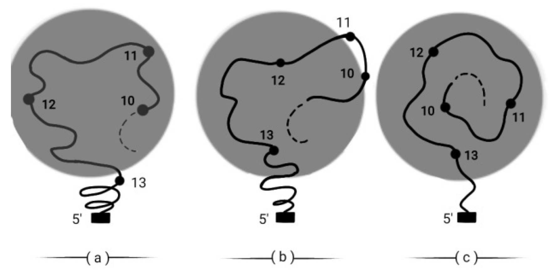
5.1 New technological advances (e.g. STORM- the stochastic optical reconstruction microscopy) made possible the measurement of quantities and properties that were inaccessible before. Physical tension in Hox clusters is such a case and more specifically the tension of DNA topological domains which are important for Hox gene activation. In D. Duboule’s Laboratory, A.R. Amàndio et al. have recently measured mouse HoxD clusters under physical tension [33]. The origin of this tension is elusive. This team has even considered the possibility of physical forces of BM to be responsible for this phenomenon. In this case they argue that ‘the forces would be generated by the local chromatin interactions themselves, rather than through an asymmetrically localized point of attachment to the nuclear environment’ [33]. Indeed this is most probable. Moreover, in the framework of BM, it is expected that in the global Hox cluster activation, there appear specific genes of the cluster (e.g. a small DNA strip containing (Hox10 and Hox11) which remain inactive for a variable time interval and they are pushed out of the Hox cluster activation domain which is depicted in the dark circle. In Figure 10a Hox10, Hox11, Hox12 are activated. In Figure 10b (Hox10, Hox11) are pushed out of the activation domain. In Figure 10c (Hox10, Hox11) reenter later in the activation domain according to the increased with the time of the BM force [34].
It is interesting that the theoretical prediction of ‘Biophysics preceds Biochemistry’ [34] was experimentally confirmed soon after ‘…structural organization of HoxD cluster may predate transcriptional activation…’ [16].
5.2 Natural Sciences are connected to the other branches of intellectual activity. A short epistemological overview is included in [40].
List of Abreviations
| AER | Apical Ectodermal Ridge |
| BM | Biophysical Model |
| CF | Coulomb Force |
| DSB | Double Strand Break |
| ER | Empirical Rule |
| FGF | Fibroblast Growth Factor |
| HGC | Hox Gene Collinearity |
| ICD | Interchromosome domain |
| Mya | Million years ago |
| PG | Paralogy Group |
| QC | Quantitative Collinearity |
| SC | Spatial Collinearity |
| TC | Temporal Collinearity |
| TFD | Transcription Factory Domain |
| wt | wild type |
Appendix 1. Symmetry in Natural Sciences
Symmetry is the cornerstone of Science and several other human intellectual activities. Many distinguished scientists have proposed their definitions of the term [35]. When an action is applied on any material object (or physical system) it causes a change. If this change leaves the system invariant, the system is symmetric. This means that any point of the system moves to another point contained in the system. I consider the compact definition of Frank Wilczek (in the form of an aphorism) is appropriate in the following context: Symmetry is a change without change [36]. The human intellect incorporates a wider realm than pure scientific thinking. Therefore, Wilczek’s definition of Symmetry could be complemented with unusual thoughts e.g. ‘Symmetry is complicated, ‘Symmetry is beautiful’ or even ‘lack of symmetry is ugly’.
Besides the obvious external symmetries in Space and Time there appeared in the last century the need to introduce several internal symmetries and particularly in the field of elementary particles with exotic names like bosons, quarks, charmed particles, mesons etc. Historically, in 1932 W. Heisenberg was the first who introduced such an esoteric term (the isotopic spin or isospin) to described the symmetry of protons and neutrons under the strong nuclear interactions [36,37].
Appendix 2. Noether’s Theory in Hox Gene Collinearity
In 1918 Emmy Noether formulated and proved in Classical Mechanics a fundamental theorem on Symmetry. In simple terms, Noether proved that a physical system obeying a symmetry law is followed by a conserved physical quantity. For example, if the physical system is invariant under time translations (that means it is independent of when is put the origin of measuring the time) the energy of the system is conserved. The significance of Noether’s theory is evident. Its application extends from the symmetry in Classical Mechanics to the complicated symmetries of elementary particle - constituents of the universe [36,37,38,39].
Among its numerous application, Noether theory was used in the study of symmetry in the important biological issue of Hox Gene Collinearity (HGC) [21]. In this case, self-similarity is the symmetry involved which is a continuous symmetry applying to all spatial lengths. The finite sequence of ordered Hox genes is the associated conserved quantity [21]. In this case, the symmetry is a ‘primitive’ self similarity since it applies to only two discrete spatial dimensions - the genome and the embryonic dimensions [20]. Consequently, PG is preserved like an irreversibly advancing ‘ratchet’ where some Hox genes are probably missing ([21], Figs 2, 3). In another biological application, Noether’s theory was recently used in a comparison of DNA sequences of different animal phylla [38].
Appendix 3. The quasi-Coulomb force
As mentioned in the Introduction, a heuristic pulling force F of BM is represented by Equation (1):
Equation (1) has the form of a quasi-Coulomb force. The proper Coulomb force (CF) is determined by the following equation
where Q1 and Q2 are the electric charges (positive or negative) and R the distance between Q1 and Q2. CF may be attractive (if one charge is positive and the other negative) or repulsive (if both charges are either positive or negative).
F = N ∗ P
CF = (Q1 ∗ Q2)/ R2
The quasi-Coulomb force F has the form
where the dependence on R is missing. The arbitrary absence of Geometry is motivated by sheer simplicity as mentioned in the Introduction. However, it turns out that this simplicity is crucial because it is related to the internal Symmetry. For example, the equations of a dynamic system are invariant under space translations. Noether proved that such a symmetric system is necessarily followed by a conserved quantity - in this case the momentum (see Appendix 2).
F = N ∗ P
In any measurement, Symmetry in a variable appears when this variable is absent in its constituent equations. In the example below, is followed the reasoning of Iliopoulos [37].
Consider a completely symmetric body (the sphere) in 3D space as described in a Cartesian system of axes (x, y, z) or a Polar coordinates system ( z, φ, θ). Any measurement in the sphere contains the angles θ and φ . It turns out that the equation of the sphere is:
where R is the radius of the sphere. In this equation, the variables (θ, φ) are indeed missing in agreement with the above symmetry requirement for Equation (4): no angular dependence is observable [37].
x2 + y2 + z2 = R2
In Equation (1’) for the quasi-Coulomb force F, the term R-2 is missing, so F is an even simpler equation than the proper Coulomb force. The meaning of this omission is that the heuristic pulling force of the BM is a quantity independent of the 3D geometric space:
F = Q1 ∗ Q2.
Note that in this space, the symmetry of F becomes internal, reminiscent of Heisenberg’s internal variable- the isotopic spin (see Appendix 1)].
References
- E.B. Lewis Nature 1978.
- S. Papageorgiou Bull. Math. Biol. 2001.
- P. Dollé et al. , Genes and Development 1991.
- S. Papageorgiou Int. J. Dev.Biol. 2006.
- B. Tarchini et al. Developmental Cell 2006.
- P. Tschopp et al. PLOS Genetics 2009.
- S. Papageorgiou Human Genetics 2009.
- S. Papageorgiou J. Dev. Biol 2021.
- D. Duboule Development 2007.
- K. Shimizu et al. PNAS 1999.
- K. Afzal et al. J. D.Biol. 2022.
- I. Simeoni et al. Dev.Biol. 2007.
- P-Y Bourillot, Development 2002.
- S. Papageorgiou Curr. Genomics 2012.
- D. Noordermeer et al. , eLIFE 2014.
- P. Fabre et al. PNAS 2015.
- P. Fabre et al. Cold Spring Harbor Lab 2015.
- A. Papantonis et al, 2005.
- P.R. Cook et al. 2018.
- S. Papageorgiou Biology 2021.
- S.Papageorgiou J. Multidiscipl. Sci. 2020.
- B.B. Mandebrot ‘The Fractal Geometry of Nature’, Editions Freeman, New York, 1982.
- S. Papageorgiou Curr. Genomics 2016.
- T. Hanscom et al. Cells 2020.
- A. Hejnol et al. PNAS 2017.
- D. Ferrier, P. Holland Mol. Phyl. Evol. 2022.
- D. E.K. Ferrier in ‘HOX GENE EXPRESSION’ Editor S. Papageorgiou, Landes Bioscience and Springer Science, USA 2007.
- D. Duboule Dev. Biol. 2022.
- M. Akam M Nature 1984.
- S. Papageorgiou Biology 2021.
- T. Kondo, D. Duboule Cell 1999.
- N. Vargesson et al. Dev. Dynamics 2001.
- A.R. Amàdio et al. Genes & Development 2021.
- S. Papageorgiou WebMedCentral+ , 2014.
- H. Weyl Symmetry, Princeton University Press 1952.
- F. Wilczek A Beautiful Question, Penguin Books, 2016.
- J. Iliopoulos Aux origines de la masse: particules élémantaires et symmétries fondamentales, Editions EDP Sciences, Paris, France, 2014.
- Y. Almirantis, A. Y. Almirantis, A. Provata, W. Li J. Mol. Evol., 2022.
- S. Merabet J Dev Biol, 2022.
- S. Papageorgiou In ‘Chaos, Information processing and Paradoxical Games’ Editors G. Nicolis – V. Basios , World Scientific, 2015.
Figure 1.
Macro-scale and Micro-scale Hox gene clustering (adapted from S. Papageorgiou, Biology 2017: 6,32). (A) Concentration (T1, T2. T3) along the Ant. - Post. Axis. (B) Time sequence (t1, t2. T3) combine with (T1, T2,T3) for expression domains of Hox1, Hox2, Hox3. (C) (bottom) a small force F1 pulls Hox1 out of the chromatin territory CT toward the Interchromosome Domain (ICD) and the Transcription Factory (TF) regime (grey domain). Polar Molecule P is opposite the telomeric end. At a later stage (top), a stronger force F3 pulls Hox1, Hox2, Hox3 out of CT in TF.
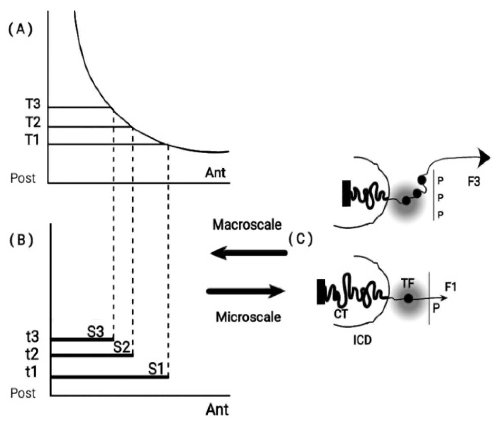
Figure 2.
Mechanical analogue of Hox cluster decondensation (adapted from S. Papageorgiou, Current Genomics 2012, 13:3). (a) (left) Before activation Hox cluster is condensed inside (CT). (right) Mechanical analogue: uncharged elastic spring fixed at its left end. (b) (left) BM pulling force decondenses the cluster and Hox1 is extruded in (ICD) in the transcription factory (TF) domain (shadow disc) The cluster is fastened posteriorily. (right) A small force F1 slightly expands the spring and black spot moves beyond the dashed line. Spring fixed posteriorily. (c) (left) Hox cluster is further decondensed and Hox1, Hox2, Hox3 move in (ICD). (right) F2> F1 and the spring is further expanded. (d) (left) The fastening of the cluster is removed and, with a smaller force F1, the cluster can slide beyond the dashed line. (right) the loose spring slides freely beyond the dashed line.
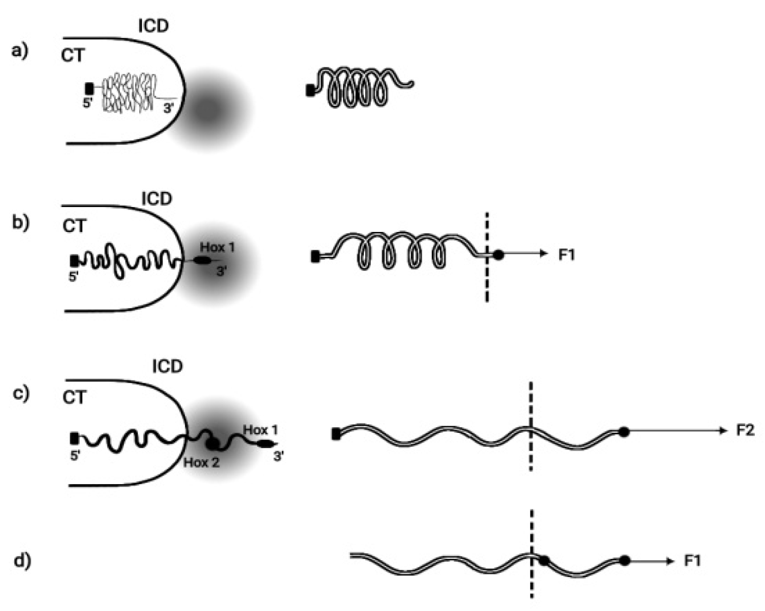
Figure 3.
Mouse Hox Gene Clusters (adapted from Z. Afzal and R. Krumlauf, J Dev Biol 2022) HoxA, HoxB, HoxC and HoxD are depicted in the direction of transcription for each gene. The mouse embryo is also shown in the Anterior – Posterior direction.
Figure 3.
Mouse Hox Gene Clusters (adapted from Z. Afzal and R. Krumlauf, J Dev Biol 2022) HoxA, HoxB, HoxC and HoxD are depicted in the direction of transcription for each gene. The mouse embryo is also shown in the Anterior – Posterior direction.
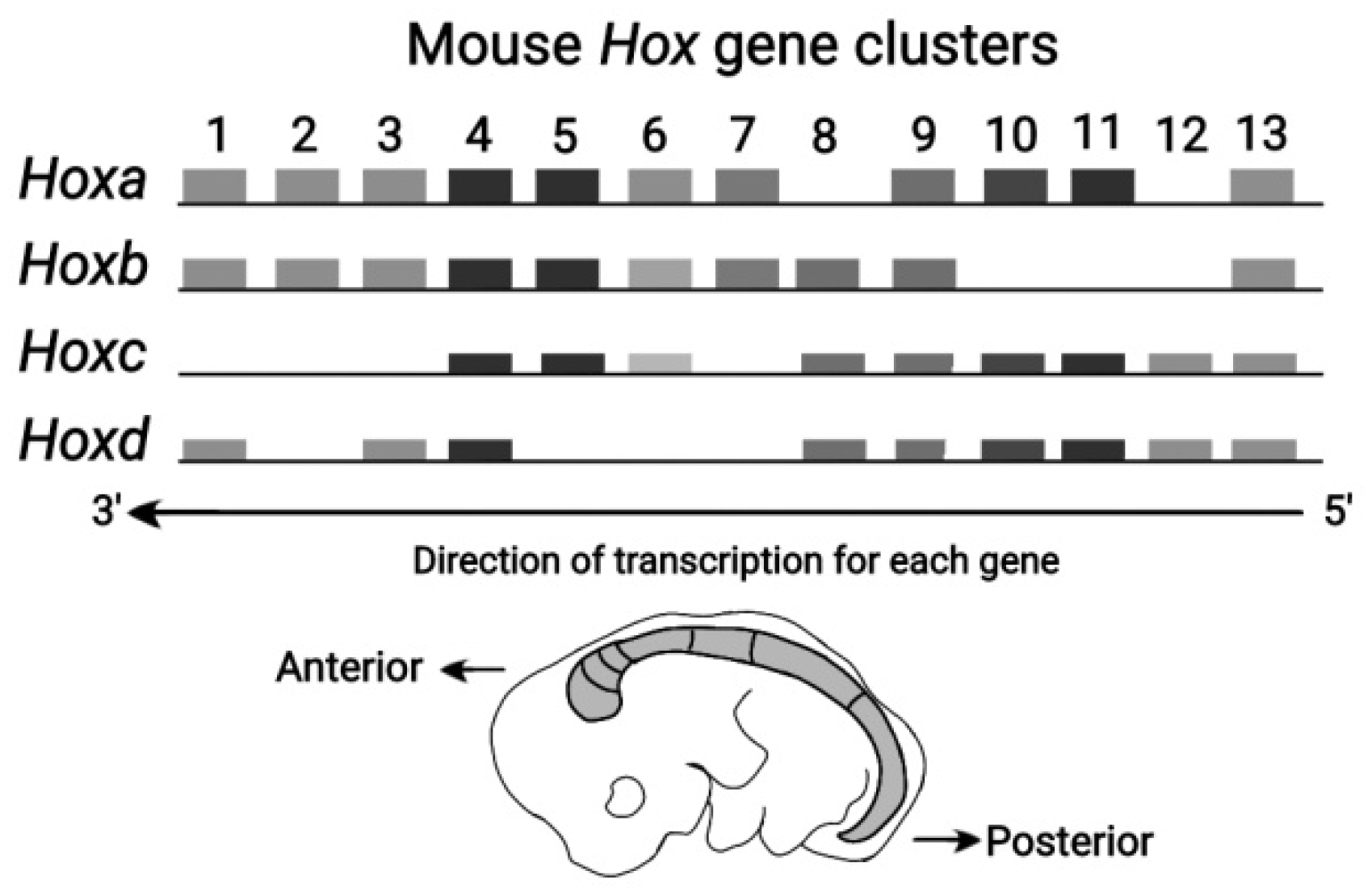
Figure 4.
A self-similar design. The Barnsley fern reproduced from Wikipedia - the free Encyclopedia.
Figure 4.
A self-similar design. The Barnsley fern reproduced from Wikipedia - the free Encyclopedia.
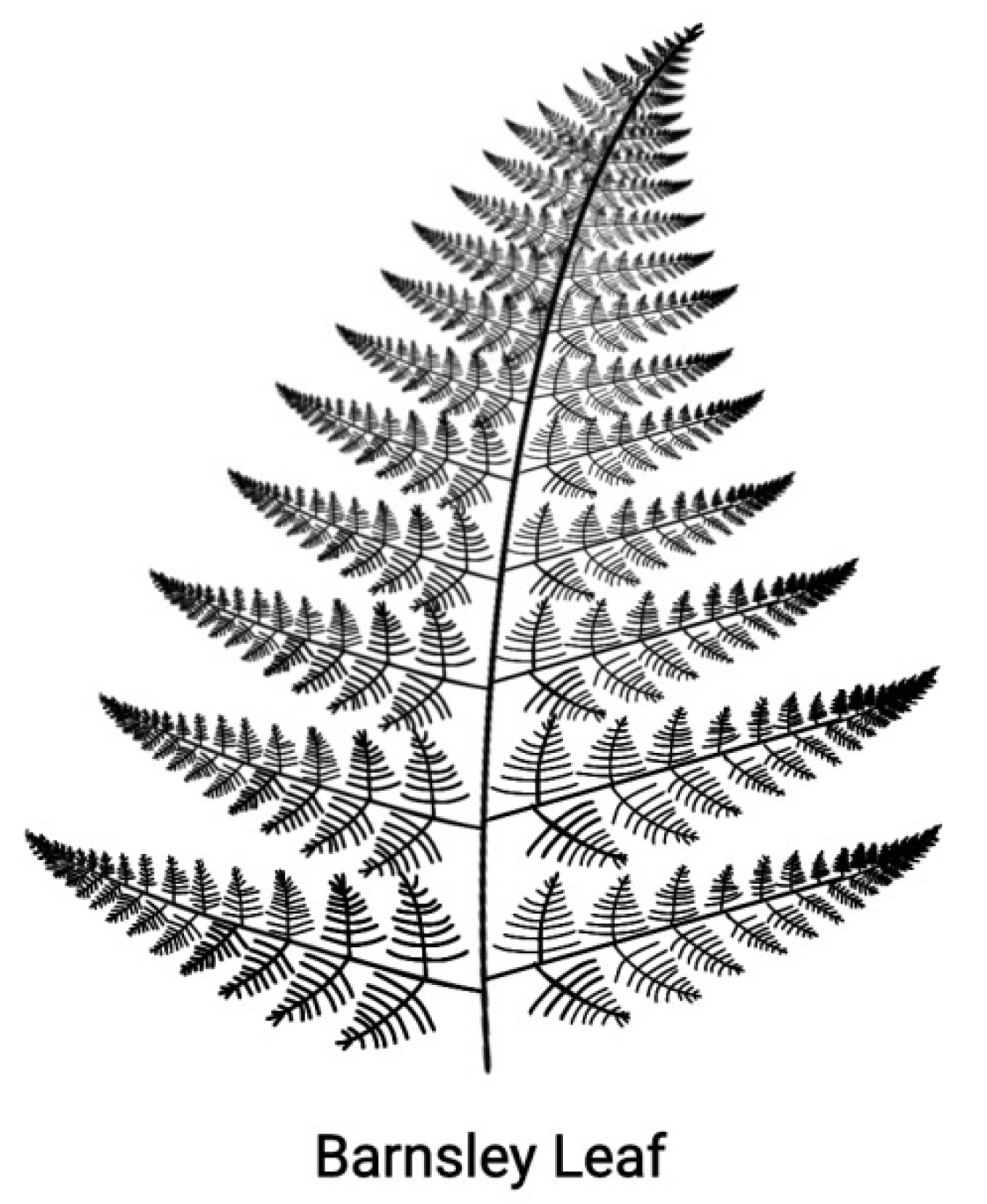
Figure 5.
Circular organization of echinoderms at different developmental stages. (A) Strongylocentratus purpuratus larva (with five podia). (B) An adult starfish (with five podia). (C) A juvenile sea urchin.
Figure 5.
Circular organization of echinoderms at different developmental stages. (A) Strongylocentratus purpuratus larva (with five podia). (B) An adult starfish (with five podia). (C) A juvenile sea urchin.
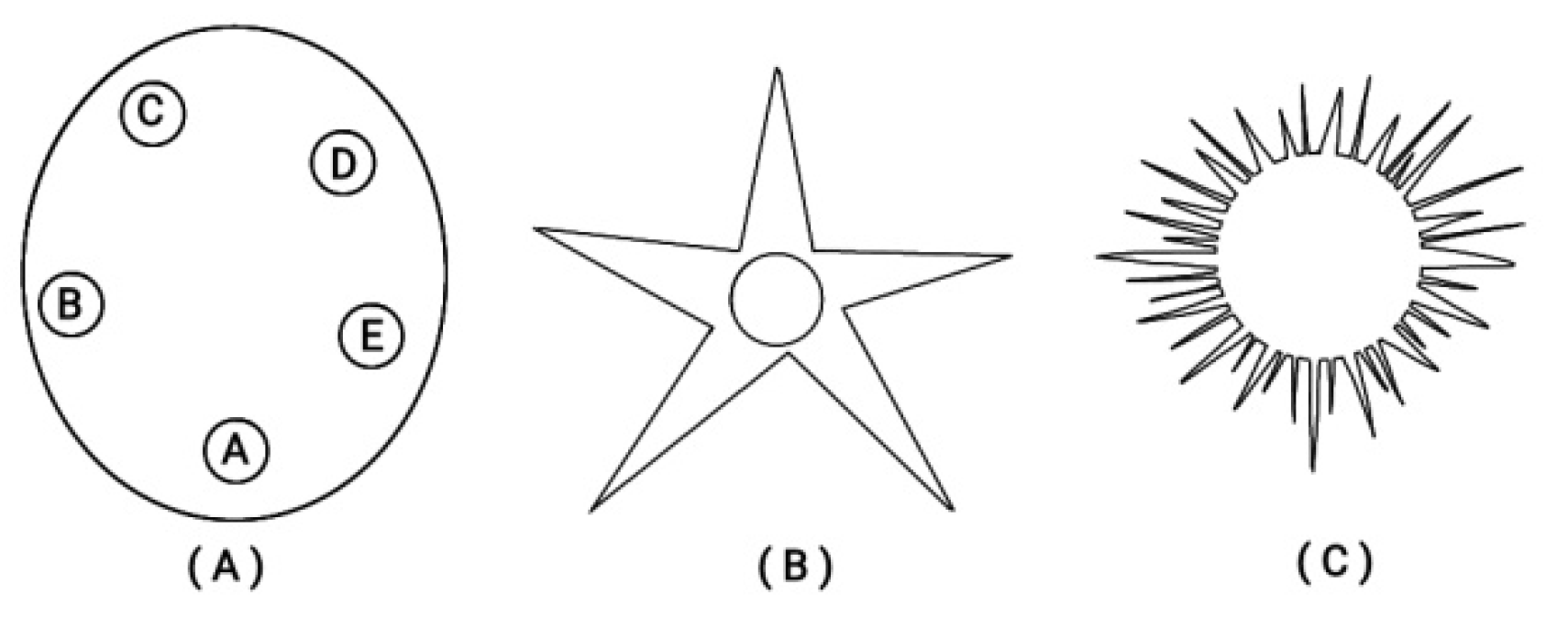
Figure 6.
Circular ordering of Hox gene clusters (adapted from S. Papageorgiou 2016, Current Genomics). (A) Bending of the 13 genes in a circle. (B) The ends of the cluster (Hox1 and Hox13) are attached to the 3’ and 5’ ends of the flanking chromosome. (C) A different attachment of Hox1 and Hox13 to the flanking chromosome. (see the text below).
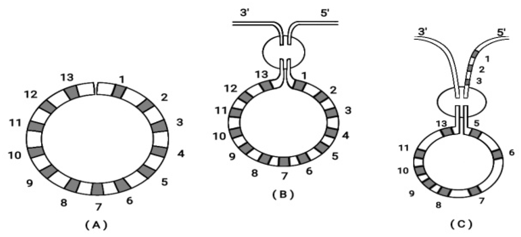
Figure 7.
(A) L Double Strand Break Left (T) and Right (C) in the middle ( INS) follows orientation (T→C) R. (B) L Double Strand Break Left (T) and Right (C) in the middle (INS) follows orientation (T←C) R
Figure 7.
(A) L Double Strand Break Left (T) and Right (C) in the middle ( INS) follows orientation (T→C) R. (B) L Double Strand Break Left (T) and Right (C) in the middle (INS) follows orientation (T←C) R
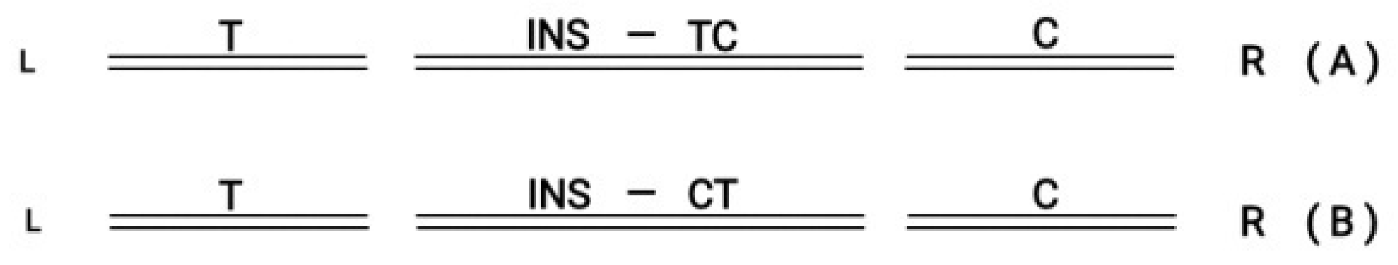
Figure 8.
The ANT-C and BX-C subclusters of Drosophila and Amphioxus (adapted from D.E.K. Ferrier in Hox Gene Expression editor S. Papageorgiou. Editions Springer and Landes Bioscience 2007).
Figure 8.
The ANT-C and BX-C subclusters of Drosophila and Amphioxus (adapted from D.E.K. Ferrier in Hox Gene Expression editor S. Papageorgiou. Editions Springer and Landes Bioscience 2007).
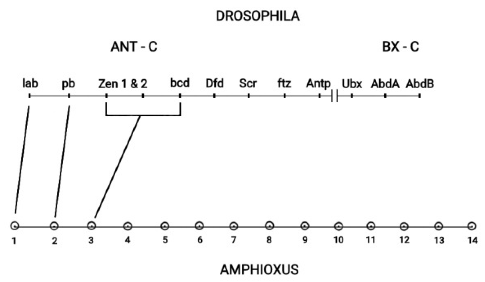
Figure 9.
Quantitative Collinearity (left) and Split clusters (right). The split clusters of section 3 and Quatitative collinearity of section 4.3 are described by identical mechanisms.
Figure 9.
Quantitative Collinearity (left) and Split clusters (right). The split clusters of section 3 and Quatitative collinearity of section 4.3 are described by identical mechanisms.
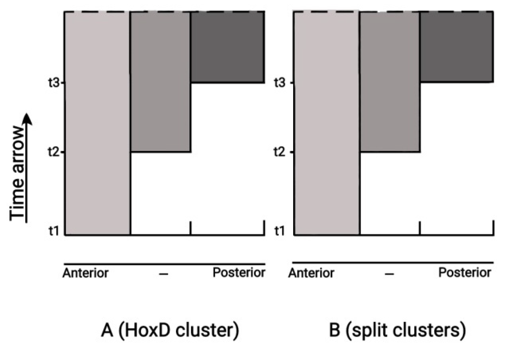
Figure 10.
A small fragmental strip of the HoxD cluster is pushed out of the cluster expression domain in (b).
Figure 10.
A small fragmental strip of the HoxD cluster is pushed out of the cluster expression domain in (b).
Disclaimer/Publisher’s Note: The statements, opinions and data contained in all publications are solely those of the individual author(s) and contributor(s) and not of MDPI and/or the editor(s). MDPI and/or the editor(s) disclaim responsibility for any injury to people or property resulting from any ideas, methods, instructions or products referred to in the content. |
© 2023 by the authors. Licensee MDPI, Basel, Switzerland. This article is an open access article distributed under the terms and conditions of the Creative Commons Attribution (CC BY) license (http://creativecommons.org/licenses/by/4.0/).
Copyright: This open access article is published under a Creative Commons CC BY 4.0 license, which permit the free download, distribution, and reuse, provided that the author and preprint are cited in any reuse.


