Submitted:
09 May 2023
Posted:
10 May 2023
You are already at the latest version
Abstract
Keywords:
1. Introduction
2. Methods
2.1. Anomaly Detection Framework
2.2. Epidemiological Feature Selection and Pre-Processing
2.3. Selecting Top-k Models for Maximum Coverage
3. Results
3.1. Anomalies by Contamination Rate
3.2. Detected Anomalies and Epidemiological Significance
3.3. Consistency and Variation in Anomaly Detected by Models
3.4. Temporal Location of Detected Anomalies
3.5. Model Selection for Inclusion in Endemic Disease Surveillance System
4. Discussion
Author Contributions
Funding
Institutional Review Board Statement
Informed Consent Statement
Data Availability Statement
Conflicts of Interest
Abbreviations
| AI | Artificial Intelligence |
| PCA | Principal Component Analysis |
| Probability density function | |
| SVM | Support Vector Machine |
References
- Health, A. Surveillance systems reported in Communicable Diseases Intelligence, 2016. Available online: https://www1.health.gov.au/internet/main/publish (accessed on 4 June 2021).
- Dash, S. , Shakyawar S.K. and Sharma M. Big data in healthcare: Management, analysis and future prospects. J. Big Data 2019, 6, 1–25. [Google Scholar] [CrossRef]
- CDC. Principles of Epidemiology in Public Health Practice, Third Edition An Introduction to Applied Epidemiology and Biostatistics. Int. J. Syst. Evol. Microbiol. 2012, ss1978. [Google Scholar]
- Felicity T., C. , Matt H. Seroepidemiology: An underused tool for designing and monitoring vaccination programmes in low- and middle-income countries. Trop. Med. Int. Health 2016, 21, 1086–1090. [Google Scholar] [CrossRef]
- Jayatilleke, K. Challenges in Implementing Surveillance Tools of High-Income Countries (HICs) in Low Middle Income Countries (LMICs). Curr. Treat. Options Infect. Dis. 2020, 1–11. [Google Scholar] [CrossRef] [PubMed]
- Nekorchuk, D.M. , Gebrehiwot T., Awoke W., Mihretie A., Wimberly M. C. Lake M. Comparing malaria early detection methods in a declining transmission setting in northwestern Ethiopia. BMC Public Health 2021, 21, 1–15. [Google Scholar] [CrossRef]
- Charumilind S., Craven M., Lamb M., Lamb J., Singhal S., Wilson M. Pandemic to endemic: How the world can learn to live with COVID-19; Mckinsey and Company 2021; pp. 1–8. Available online: https://www.mckinsey.com/industries/healthcare-systems-and-services/our-insights/pandemic-to-endemic-how-the-world-can-learn-to-live-with-covid-19.
- Clark J., Liu Z., Japkowicz N. Adaptive Threshold for Outlier Detection on Data Streams. In Proceedings of the 2018 IEEE 5th International Conference on Data Science and Advanced Analytics (DSAA) 2018; pp. 41–49. [CrossRef]
- hao M., Chen J.,Li Y. A Review of Anomaly Detection Techniques Based on Nearest Neighbor. In Proceedings of the 2018 International Conference on Computer Modeling, Simulation and Algorithm (CMSA 2018); 2018; 151, pp. 290–292. [CrossRef]
- Hagemann T., Katsarou K. A Systematic Review on Anomaly Detection for Cloud Computing Environments. In Proceedings of the 2020 ACM 3rd Artificial Intelligence and Cloud Computing Conference; 2021; pp. 83–96. [CrossRef]
- Turing, A.M. Computing Machinery and Intelligence. Mind 1950, 49, 433–460. [Google Scholar] [CrossRef]
- Bitterman D.S, Miller T.A, Mak R.H, Savova G.K. Clinical Natural Language Processing for Radiation Oncology: A Review and Practical Primer. Int. J. Radiat. Oncol. Biol. Phys. 2021, 110, 641–655. [CrossRef]
- Baroni, L. et al. An integrated dataset of malaria notifications in the Legal Amazon. BMC Res. Notes 2020, 13, 1–3. [CrossRef]
- Baena-garcia M., Campo-avila J.D, Fidalgo R., Bifet A., Gavalda R., Morales-Bueno R. Early drift detection method. In Proceedings of the Fourth International Workshop on Knowledge Discovery from Data Streams 2006; pp. 1–10. Available online: https://www.cs.upc.edu/ abifet/EDDM.pdf.
- Weaveworks. Building Continuous Delivery Pipelines Deliver better features, faster. Weaveworks Inc. 2018; pp. 1–26. Available online: https://www.weave.works/assets/images/blta8084030436bce24/CICD_eBook_Web.pdf.
- Shereen M.A., Khan S., Kazmi A., Bashir N., Siddique R. COVID-19 infection: Origin, transmission, and characteristics of human coronaviruses. J. Adv. Res. 2020, 24, 91–98. [CrossRef]
- Ali, M. PyCaret: An open source, low-code machine learning library in Python. PyCaret version 1.0.0 2020, 24. [Google Scholar]
- Schubert E, Wojdanowski R., Kriegel H.P. On Evaluation of Outlier Rankings and Outlier Scores. In Proceedings of the 2012 SIAM International Conference on Data Mining 2012; pp. 1047–1058. [CrossRef]
- Tang J., Chen Z., Fu A.W., Cheung D.W. Enhancing Effectiveness of Outlier Detections for Low Density Patterns In: Chen MS., Yu P.S., Liu B. (eds) Advances in Knowledge Discovery and Data Mining. Lecture Notes in Computer Science 2002, 2336, 535–548. [CrossRef]
- Akshara. Anomaly detection using Isolation Forest – A Complete Guide. Analytics Vidya 2021, 2336, 1–10. [Google Scholar]
- Goldstein M. and Dengel A. Histogram-based Outlier Score (HBOS): A fast Unsupervised Anomaly Detection Algorithm. Conference paper 2012, 1–6. Available online: https://citeseerx.ist.psu.edu/viewdoc/download?doi=10.1.1.401.5686&rep=rep1&type=pdf.
- Gu X., Akogluand L., Fu A.W, and Rinaldo A. Statistical Analysis of Nearest Neighbor Methods for Anomaly Detection. 33rd Conference on Neural Information Processing Systems (NeurIPS 2019), Vancouver, Canada. 2019, 1 – 11. Available online: https://proceedings.neurips.cc/paper/2019/file/805163a0f0f128e473726ccda5f91bac-Paper.pdf.
- Tax, D.M. J and Duin R.P.W. Support Vector Data Description. Machine Learning 2004, 54, 45–66. [Google Scholar] [CrossRef]
- McCaffrey J. Anomaly Detection Using Principal Component Analysis (PCA). The Data Science Lab,The Visual Studio Magazine 2021, 582–588. Available online: https://visualstudiomagazine.com/articles/2021/10/20/anomaly-detection-pca.aspx. /.
- Fauconnier C., Haesbroeck G. Outliers detection with the minimum covariance determinant estimator in practice. Statistical Methodology 2009, 6, 363–379. [CrossRef]
- Janssens J.H.M. Outlier selection and One-class classification. Ph.D thesis, Tilburg Universityy, Netherlands 2013, 59–95. Available online: https://github.com/jeroenjanssens/phd-thesis/blob/master/jeroenjanssens-thesis.pdf.
- Chandu, D.P. Big Step Greedy Heuristic for Maximum Coverage Problem. International Journal of Computer Applications (0975 – 8887) 2015, 125, 19–24. [Google Scholar]
- Jaramillo-Valbuena S.,Londono-Pelaz J.O., Cardona S.A. Performance evaluation of concept drift detection techniques in the presence of noise. Revista 2017, 38, 1–10.
- Geyshis D. 8 Concept Drift Detection Methods. Aporia 2021, 1–5. Available online: https://www.aporia.com/blog/concept-drift-detection-methods/.
- Farrington C.P., Andrews N.J, Beale A.J., Catchpole D. A statistical algorithm for the early detection of outbreaks of infectious disease. Journal of the Royal Statistical Society Series, Rockefeller University Press 1996, 159, 547–563.
- Noufaily A., Enki D.G., Farrington P., Garthwaite P., Andrews N. and Charlett A. An improved algorithm for outbreak detection in multiple surveillance systems. Stat. Med. 2012, 32, 1206–1222. [CrossRef]
- Abdiansah A; Wardoyo R. Time Complexity Analysis of Support Vector Machines(SVM) in LibSVM. Int. Comput. Appl. 2018, 128, 28–34.
- Shweta, B.; Gerardo, C.; Lone, S.; Alessandro, V.; Cécile, V.; Lake, M. Big Data for Infectious Disease Surveillance and Modeling. J. Infect. Dis. 2016, 214, s375–s379. [Google Scholar] [CrossRef]
- Kovacs, G.; Sebestyen, G.; Hangan, G. Evaluation metrics for anomaly detection algorithms in time-series. Acta Univ. Sapientiae Inform. 2019, 11, 113–130. [Google Scholar] [CrossRef]
- Antoniou, T.; Mamdani, M. Evaluation of machine learning solutions in medicine. Analysis CPD 2021, 193, 41–49. [Google Scholar] [CrossRef] [PubMed]
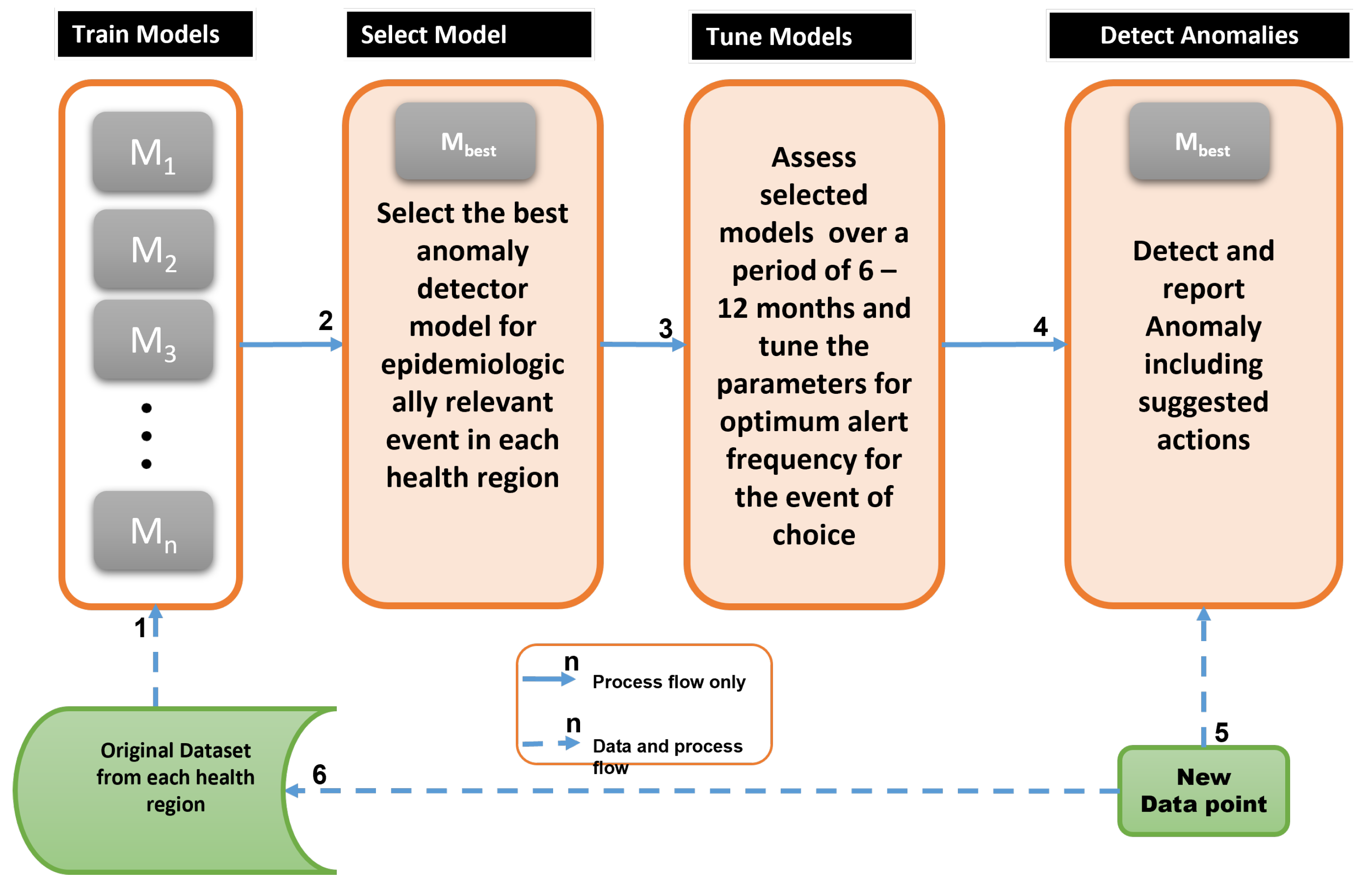


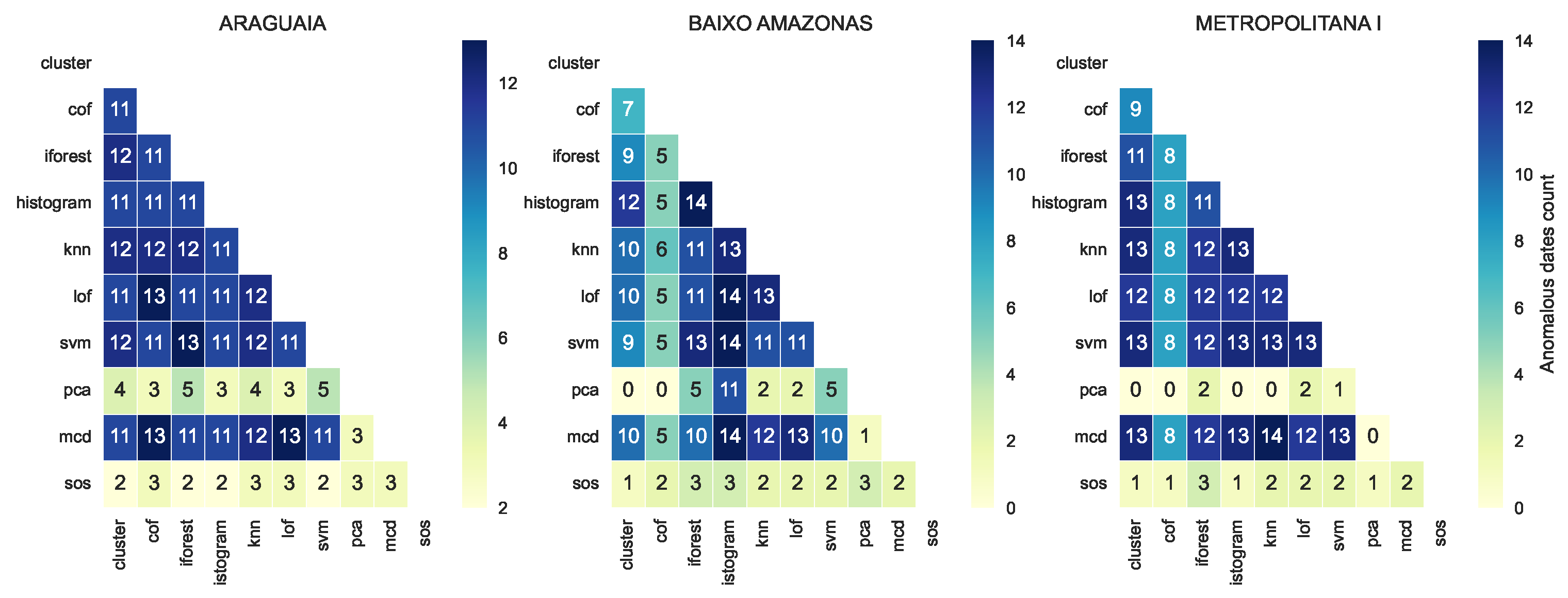
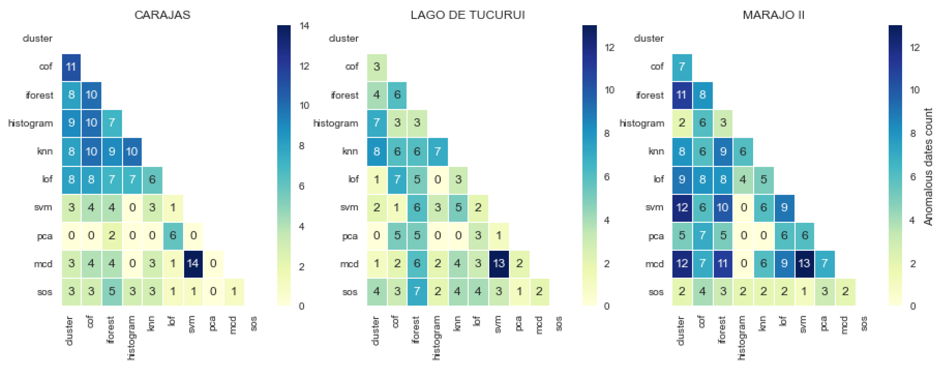
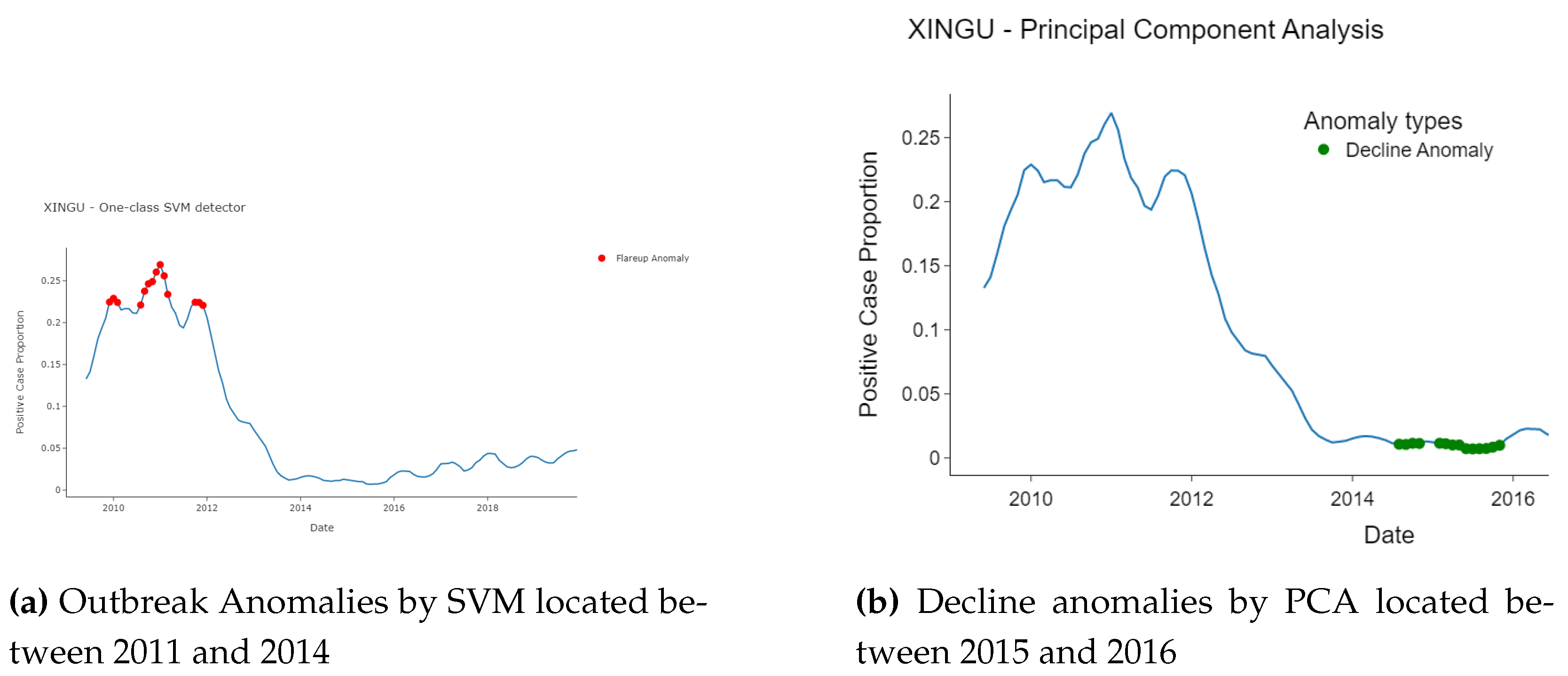
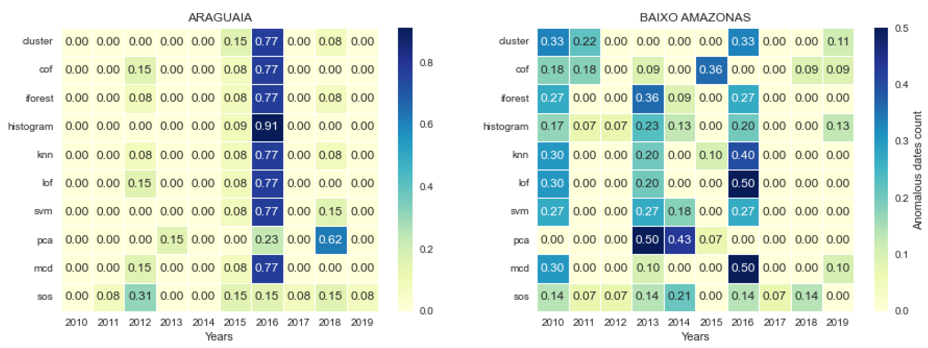
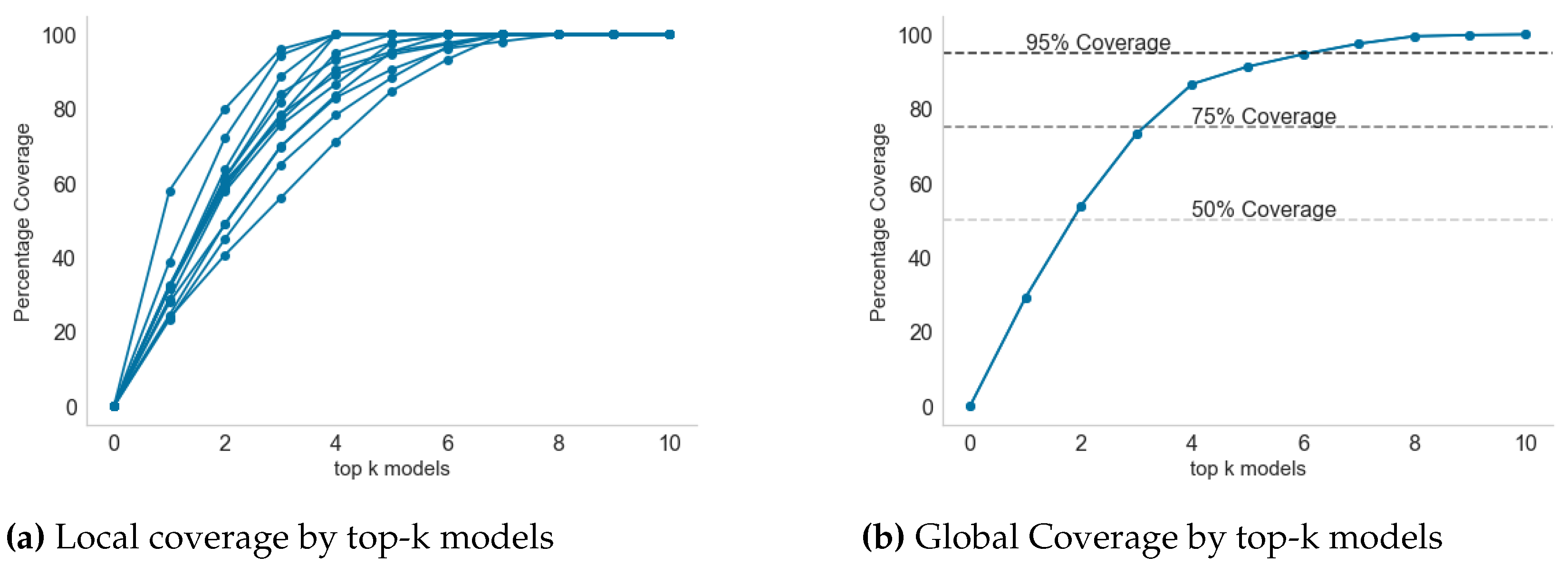
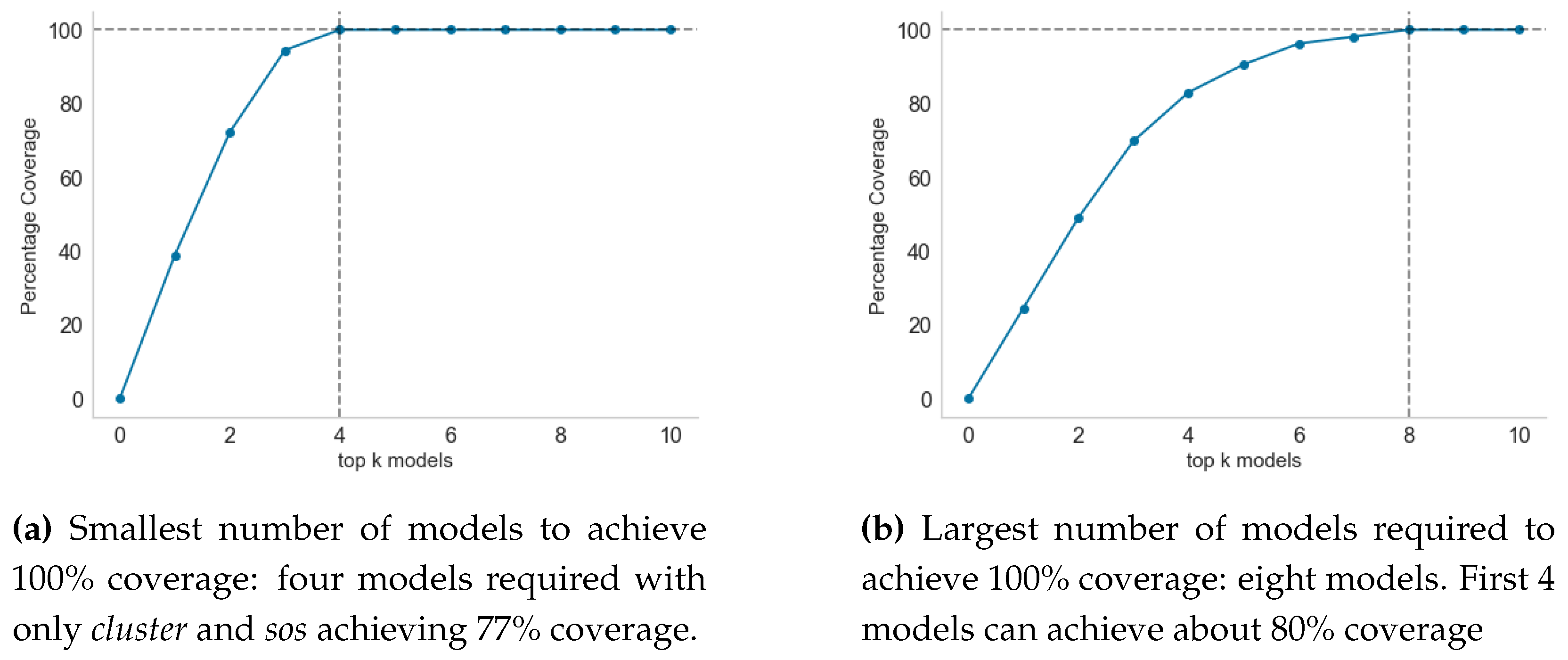
| Step No. | Major activities |
|---|---|
| 1 | Train candidate anomaly detectors per health region using train set |
| 2 | Based on local epidemic demands, select best anomaly detector, |
| 3 | Tune model parameters after using for 6 - 12 months to evaluate performance |
| 4 | As new data arrives, use the best detector, to detect and interpret anomaly |
| 5 | New data for evaluation and model re-training |
| 6 | Update the models with the new data and repeat from Step 1 |
| No. | Model ID. | Model Name | Core Distance measure |
|---|---|---|---|
| 1 | cluster | Clustering-Based Local Outlier [18] | Local outlier factor |
| 2 | cof | Connectivity-Based Local Outlier [19] | average chaining distance |
| 3 | iforest | Isolation Forest [20] | Depth of leaf branch |
| 4 | histogram | Histogram-based Outlier Detection [21] | HBOS |
| 5 | knn | K-Nearest Neighbors Detector [22] | Distance Proximity |
| 6 | lof | Local Outlier Factor [18] | Reacheability distance |
| 7 | svm | One-class SVM detector [23] | hyper-sphere volume |
| 8 | pca | Principal Component Analysis [24] | Magnitude of reconstruction error |
| 9 | mcd | Minimum Covariance Determinant [25] | Robust distance from MCD |
| 10 | sos | Stochastic Outlier Selection [26] | Affinity probability density |
Disclaimer/Publisher’s Note: The statements, opinions and data contained in all publications are solely those of the individual author(s) and contributor(s) and not of MDPI and/or the editor(s). MDPI and/or the editor(s) disclaim responsibility for any injury to people or property resulting from any ideas, methods, instructions or products referred to in the content. |
© 2023 by the authors. Licensee MDPI, Basel, Switzerland. This article is an open access article distributed under the terms and conditions of the Creative Commons Attribution (CC BY) license (http://creativecommons.org/licenses/by/4.0/).


