Social Network Analysis in Forestry Projects

Preprint

Article

Social Network Analysis in Forestry Projects

Altmetrics

Downloads

108

Views

Comments

Adrienn Novotni,Zoltán Pásztory,

Zsolt Tóth^*

Adrienn Novotni,Zoltán Pásztory,

Zsolt Tóth^*

This version is not peer-reviewed

Submitted:

10 May 2023

Posted:

11 May 2023

You are already at the latest version

Alerts

Abstract

Using SNA techniques, the study examined H2020 forestry projects. An adjacency matrix was created using the CORDIS data collection, and it was then utilized to depict the network of project members. Then, different network indicators were computed. Several statistical techniques (maximum likelihood, Kolmogorov-Smirnov test, moments, bootstrapping) were employed to do a goodness-of-fit analysis on the frequencies of the degrees to confirm scale-freedom or randomness in the search for significant distributions in network research. Additionally, the small-world aspect was investigated. The findings demonstrate that while the number of project participations by project participants follows a power distribution, the distribution of project participants’ degrees reflects various effects. As a result, the scale-freedom that has been emphasized in many scientific investigations is not evident. The network indicators demonstrate that the network is not clearly small-world.

Keywords:

Subject: Social Sciences - Other

1. Introduction

This paper's analysis is an illustration of SNA (Social Network Analysis). Using network research methodologies, the primary study goal is to construct and analyze networks of organizations, academic institutions, and businesses, mostly from Europe, that are involved in Horizon2020 projects forestry.

The various network indicators will gauge the network's "growth," or how "effectively" it connects individuals and how much information and knowledge exchange is facilitated. For companies, research centers, and other forestry actors, this information is unquestionably crucial and can show the way forward. The degree (number of contacts) of the network participants was the focus of the investigation. The various degree number distributions may reveal information about the networks' nature, structure, and logic of operation. Because few nodes typically have many degree numbers or numerous nodes typically have few degree numbers in many spheres of social interaction, the study of scale-freedom is crucial. Forestry businesses, research institutions, and other actors have a right to wish to interact with the key players in networks while raising R&D funds, especially in the case of scale-free networks.

Since the second part of the 1990s, the study of social networks has received significant academic interest after several predecessors. It is largely because of Albert-László Barabási's [1] works. Worldwide, Barabási has made significant contributions to the field, particularly in the areas of science management and the IT implementation of current theories [2]. However, network analysis had been a significant area of study for many years before to it, beginning to mature in the latter half of the 1950s. The methods of network analysis used in this research expand on the findings of recent decades. We therefore employed the outcomes of the models defining random networks/graphs [3], the configuration model for networks made of entirely random links, but with a defined degree number distribution [4,5,6], the small world model [7], and the scale-free network model [8].

A well-established methodology exists for network analysis. Some of the techniques have ties to various theoretical schools of thought, although when viewed theoretically, they can be seen more as a "pattern" with a certain logic.

2. Materials and Methods

First, a usable relational database was created using the CORDIS downloaded dataset. The database can be used to retrieve information from every Horizon 2020 project.

Utilizing search criteria, forestry projects were pre-selected, and the dataset was then further reduced through the use of content analysis.

The forestry is featured in 254 of the 30,084 Horizon 2020 projects. Of the 1,340 project participations, 397 were higher or secondary education establishments, 340 were research organisations, 320 were private for-profit entities, 149 were public bodies, and 134 were other organisations. The participants represent 62 countries, 28 (all member states before Brexit) from the European Union. The top 5 countries involved in most projects are Germany (138), Spain (135), Italy (121), United Kingdom (100), and France (100).

The direction of connection between nodes in the network of the forestry project is ignored, so it is viewed as an undirected network. Scientific collaborations are regarded of as undirected links, regardless of their varied statuses. For instance, we didn't take the participant's role as a project coordinator into account.

The vectors needed to store each pair of connections were first created. We initially produced a matrix using this data, and then an undirected graph. The adjacency matrix must be built as the next stage. In network research, the adjacency matrix is crucial. We created the link network using the adjacency matrix. The number of connections in a network can be recorded in the formula

PE = \frac{N (N - 1)}{2}

(1)

where N is the number of network elements. An undirected network's density can be expressed as

D = \frac{2 E}{N (N - 1)}

(2)

where E represents the number of edges. The density is 1 if all possible connections exist and everyone is connected to everyone else. No one is connected to anyone with a density of 0. As a result, the density value is a number ranging from 0 to 1, with higher values signaling more network density [9].

The average probability is defined as transitivity. If one node is linked to another, and that node is linked to a third, then our initial node is also linked to the third node [10]. Transitivity is often referred to as the average clustering coefficient, which may be calculated using the clustering coefficient (the transitivity of a given node) [11]. The i-th node's clustering coefficient with degree k_i is

C_{i} = \frac{2 L_{i}}{k_{i} (k_{i} - 1)}

(3)

where L_i is the number of links between the i-th point's neighbours with k_i degrees. It always has a value between 0 and 1. The overall network's average clustering coefficient is

C = \frac{1}{N} \sum_{i = 1}^{N} C_{i}

(4)

according to the clustering coefficient. The total number of connections can be calculated using the number of nodes (N) and the number of degrees (k) with the formula

L = \frac{1}{2} \sum_{i = 1}^{N} k_{i}

(5)

in a network that is undirected.

The ability of a network to be characterized as scale-free is a basic feature. If the degree distribution of a network can be characterized by a power function, it is said to be scale-free [11]. The moments of the degree distribution express the essence of scale-free networks. The degree number distribution's n-th moment is

k^{n} = \int_{k_{m i n}}^{k_{m a x}} k^{n} p (k) d k = C \frac{k_{m a x}^{n - γ + 1} - k_{m i n}^{n - γ + 1}}{n - γ + 1}

(6)

in scale-free networks. True scale-free and random networks (normal or Poisson distribution) are uncommon, and most existent networks are formed and evolve because of a range of effects. As a result, a critical challenge in network research is whether we can represent the frequencies of degree numbers using a distribution other than random (Poisson or normal) or power distribution. This question falls within the category of goodness-of-fit analysis in statistics. However, we must clarify two seemingly insignificant things about degrees.

The first issue is deciding whether to treat the number of degrees per node as a discrete or continuous variable. The number of degrees is obviously a discrete variable, but in the case of a larger network or more active cooperation, it may be substantially greater or much more diverse than the current one. Furthermore, the variable changes on a proportionate scale. In such instances, popular statistical software, for example, introduces the concept of a "discrete variable handled as a continuous variable" and advises that the discrete variable be analyzed using continuous analysis methods [12,13].

The authors of the fitdistrplus distribution fitting package and associated vignette treat discrete variables with numerous elements as continuous [14]. However, the application of continuous approaches to discrete variables for fit analysis methods for more typical distributions is debatable [15].

A similar issue was deciding whether to employ population or sample statistical methods in the analysis. The difficulties in defining some forestry project features as a population, the not-always-complete project network, and the intrinsically imperfect nature of data collecting require the use of approaches that "manage" uncertainties and imperfections, such as bootstrapping methods in our situation. If we view the set of forestry projects registered in Horizon 2020 as a population, the project network that we are exploring as a possible representation of all possible project networks or as a possible sample of forestry projects creates far more serious sampling difficulties. As a result, we tended to favor the latter throughout the analysis. Nonetheless, we followed the recommendations in the literature and ran the relevant statistical tests.

In that instance, the standard goodness-of-fit test question may be adjusted. It is not essential to estimate whether the population in the sample satisfies the specified distribution, but rather to assess whether the population itself satisfies the supplied distribution (with methodological caveats and caution). This is not a major issue if you are not seeking for specific parameters and simply want to confirm or reject your fit hypothesis [14,15,16]. Naturally, all such contentious methodological concerns should be treated with extreme caution. We aimed to select methods that produce accurate findings for nearly "every" data set while excluding approaches that produce huge deviations.

We used a discrete variable approach to determine whether the data series follows a Poisson distribution. A χ² test or a maximum likelihood method can (and was) used to test for a Poisson distribution. The approach chosen can be applied to both a sample and a group believed to be a population. We also examined if the degree numbers follow a power distribution. Because of the uncertainty in calculations, it is worthwhile to use bootstrapping methods with greater machine needs. The bootstrapping approach performs several back-sampling and estimate procedures on the data set under consideration before accumulating the results.

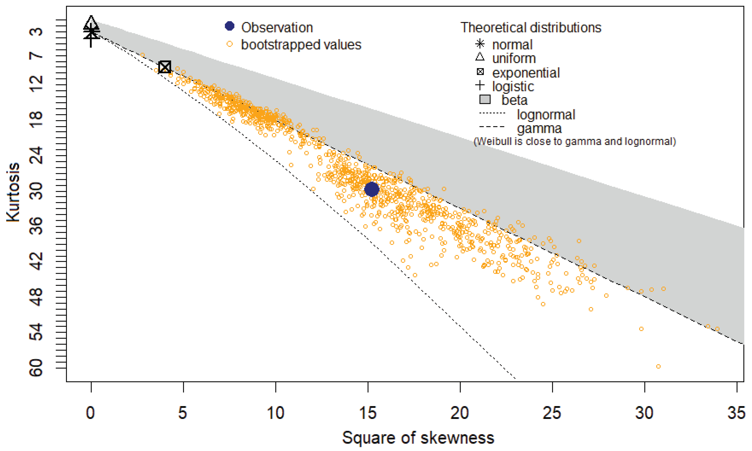
In most cases, the chosen computer algorithm is employed for sampling methods. We have not changed the sample technique because we are treating the group as a population, and the algorithm handles this well. Otherwise, the difference between the two outcomes would be negligible. A Cullen-Frey diagram (Kurtosis-Skewness diagram) illustrating the possible values for the most common distributions was also created [17]. We chose a non-parametric (non-normal) bootstrapping approach with boot = 1000 since skewness and kurtosis are not robust (little parameter changes can result in big alterations) [18]. This process produces consistent and visually appealing outcomes. For both discrete and continuously treated discrete variables, the graph was generated.

Diameter is the network's "path length": the number of steps required to travel from one node to any other node through the shortest available route. Little-diameter networks are referred to as "small worlds" [19]. The formula

d_{\max} \approx \frac{\ln N}{\ln 〈 k 〉}

(7)

describes a network's diameter. The small-world phenomenon is described by equation (7) [11]. Because equation (7) approximates the average distance (〈d〉) between two randomly chosen nodes better than d_max in most networks, the formula

d \approx \frac{\ln N}{\ln 〈 k 〉}

(8)

describes the small-world phenomenon. Thus, "small" for a small-world network means that the average path length or diameter varies logarithmically with network length.

Betweenness is a measure of how important an actor's network location is for network cooperation and information flow. If a node is located on multiple paths that are the shortest distance between two other actors, it is likely to play an important role in the network [20,21].

The betweenness of a v node is

g (v) = \sum_{s \neq v \neq t} \frac{σ_{st} (v)}{σ_{st}}

(9)

where σ_st is the number of shortest paths between nodes s and t, and σ_st(v) is the number of paths that pass through v. For undirected graphs, the normalized form is frequently used, in which the expression (9) is divided by (N-1)(N-2)/2. The expression

normal (g (v)) = \frac{g (v) - \min (v)}{\max (v) - \min (v)}

(10)

is also frequently used in its normalized form. In both cases, the value is within the [0.1] range. The number of degrees and the betweenness can be used to filter out the most important participants. Many other indicators can be calculated using the literature, but this article only includes the most important ones for analysis.

3. Results

3.1. Creating the network of connections

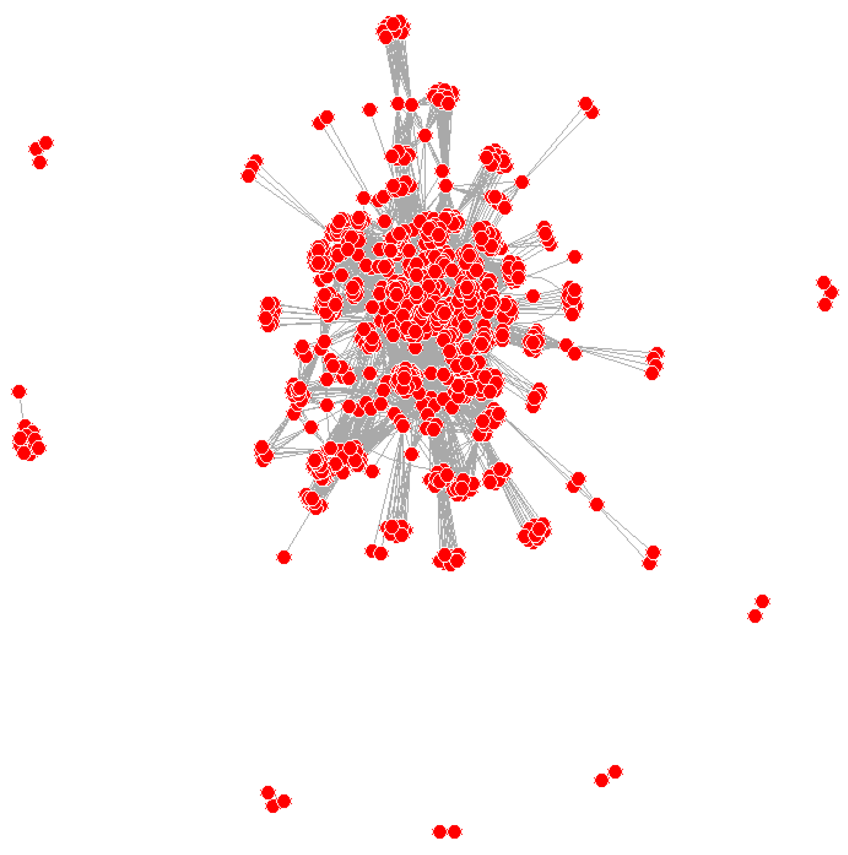
The adjacency matrix yields an 817-row and 817-column matrix. As a result, the total number of nodes is 817. Figure 1 depicts the network of connections between project participants based on the adjacency matrix.

The mapped network of connections reveals little about the network's nature. It does show that most project participants are connected, but there are also peripheral groups and participants.

3.2. Calculated network indicator values and fit test results

According to equations (1,2), the density is 0.035. The values of networks of similar size and type would be required for a reliable evaluation of the result. The value does not appear to be high. There could be two reasons for this. Perhaps the connections between forestry institutions, research institutes, and businesses are underdeveloped. However, the studied networks are more likely to describe the forestry's R&D-intensive elite. Because resources are limited, the number of project participants clearly lags far behind the number of potential participants.

The calculated transitivity from equations (3,4) is 0.59, which is also subject to the uncertainty indicated in the previous indicator. Despite the uncertainty, this value appears to be high, indicating that the "my friend's friend is my friend" phenomenon is quite prevalent in the forestry project network. This implies that forestry project participants are essentially the "top" of the forestry and are typically connected through established contacts, which is unfortunate for outsiders.

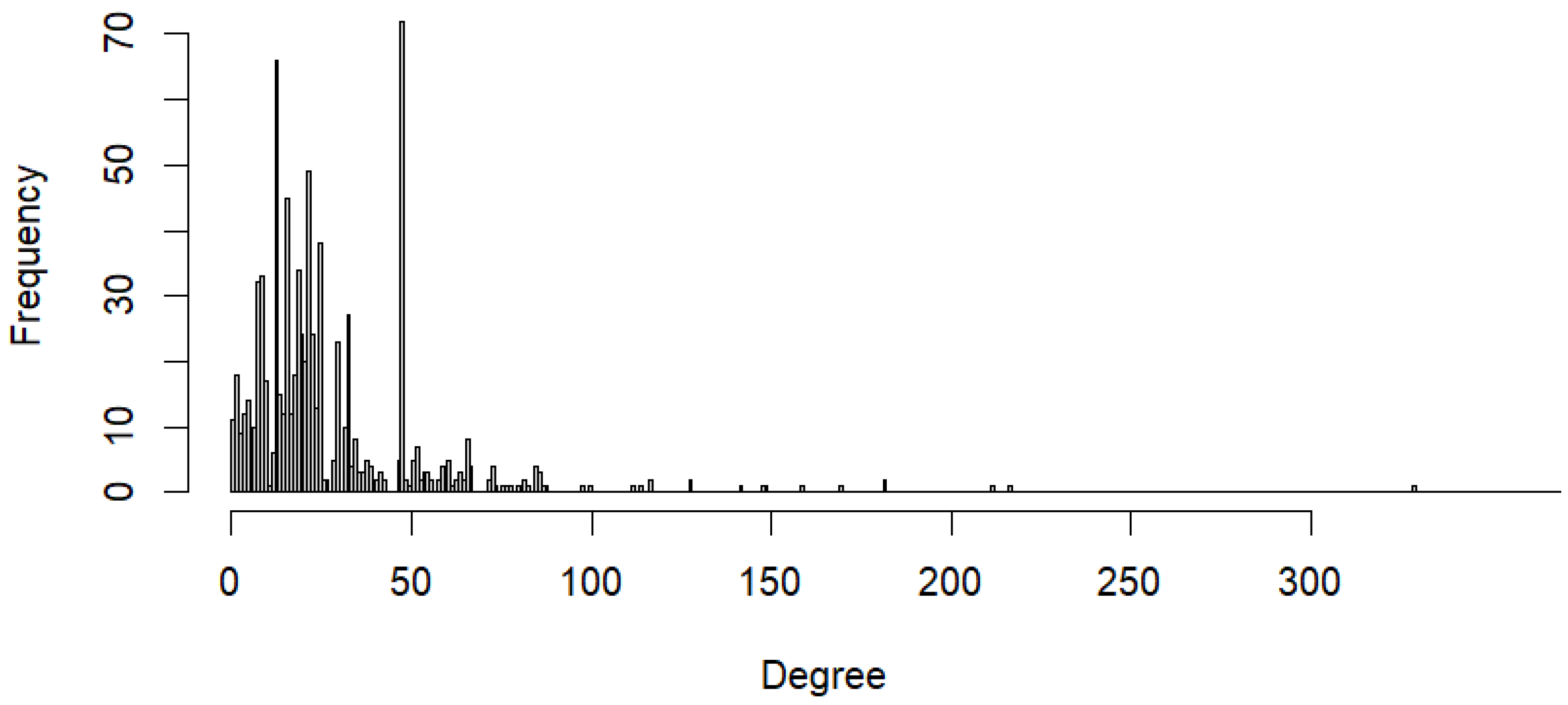
Figure 2 depicts the degrees obtained from the equation (5). The maximum likelihood estimation of Poisson distribution yielded the following results: G² = 13079.2, df = 86, p = 0, λ = 28.34. In the case of α = 0.05 c_crit = 108.65 G² > c_crit and p < α; therefore, H₀ is rejected. The degree numbers are not Poisson distributed.

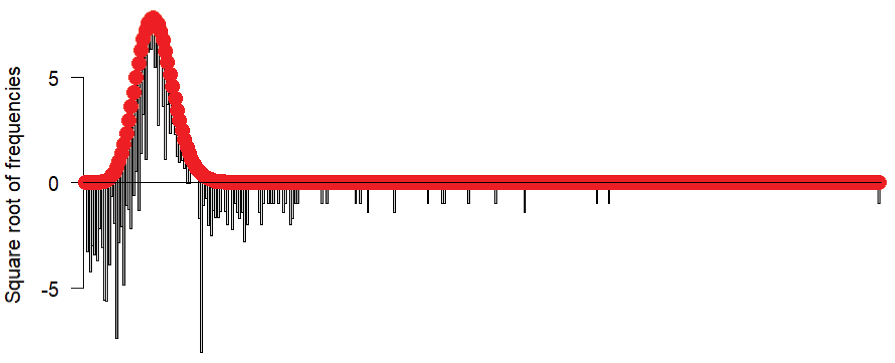
The rootogram, which shows how far our empirical values should be shifted to achieve the desired distribution, validates our findings (Figure 3).

According to a Poisson distribution of degree numbers, most participants would have had average degrees. It is presumptive that no one would hold a distinctive position among the participants in these networks. We would discover nodes of equal rank by looking at how a network formed from such locations. The findings imply that this can be totally ruled out because the forestry project network obviously contains nodes with privileged responsibilities. This supports our earlier findings.

The following values were obtained from the goodness-of-fit (power distribution) test: α = 3.48, x_min = 51, p = 0.85. Perhaps, we should accept H₀ given the large p-value obtained, however this would be the incorrect conclusion. Because it is obvious that our empirical values for x ≥ 51 follow a power distribution, H₀ is therefore rejected.

The 1000-iteration bootstrapping procedure yielded the following values: α = 3.40, x_min = 48, p = 0.27. The large change in p is due to a single value. H₀ is rejected as a result, because the data series can be categorized as power-distributed with slightly different x_min. But that x_min value is too high as well.

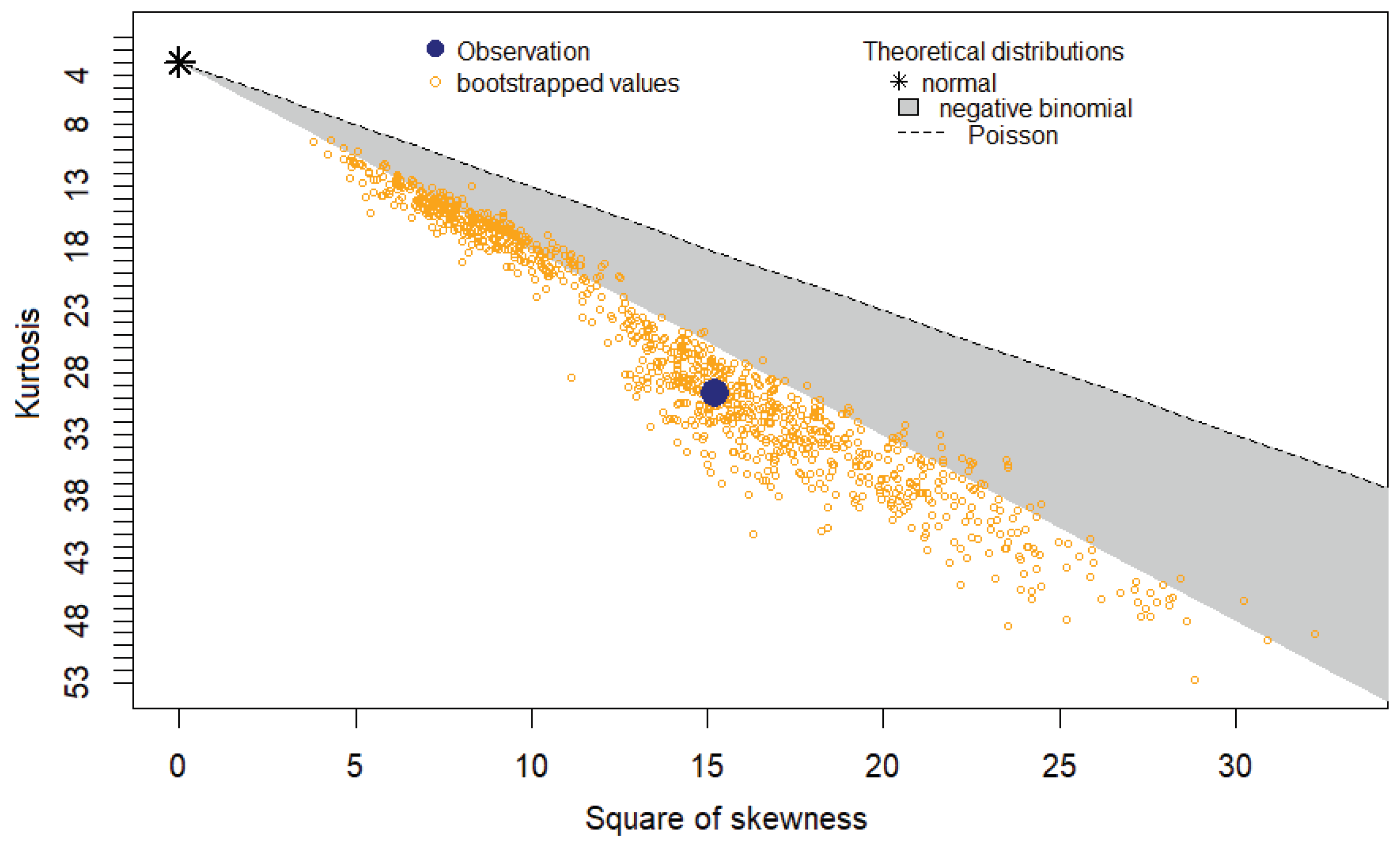
We may also test the potential distribution of the degree numbers using the Cullen-Frey diagram. Our earlier findings are supported by the discrete variable's Cullen-Frey plot, which shows that it does not follow a Poisson distribution. Additionally, it does not fall within the negative binomial distribution's range (Figure 4).

The distribution of the degree numbers is shown to lie between the gamma and lognormal distributions and outside the range of the beta distribution in the Cullen-Frey diagram (Figure 5) for the discrete variable treated as a continuous variable. A high peak is indicated by a kurtosis value that is substantially greater than 3. As with the other three "skewed" distributions, the fit of the Weibull distribution is constrained in this situation. Other than the Poisson and power distributions, certain regularities that are uncommon in economic and social processes can be suggested, but this does not seem to be the case in this instance.

Based on the data, we can infer — and this is the most plausible inference — that a mix of random and scale-freedom-promoting factors contributed to or formed the "skewed to the left" distribution. The nature of the search for project partners can also be used to infer the outcome. The frequency of the lowest degree numbers was inevitably lower than in scale-free networks because as the network expanded, participants tended to prefer to connect to nodes that were already recognized or had many network connections at the submission stage (preferential connection). However, this also brought them into contact with other project participants. Additionally, the funding program favors projects including numerous actors.

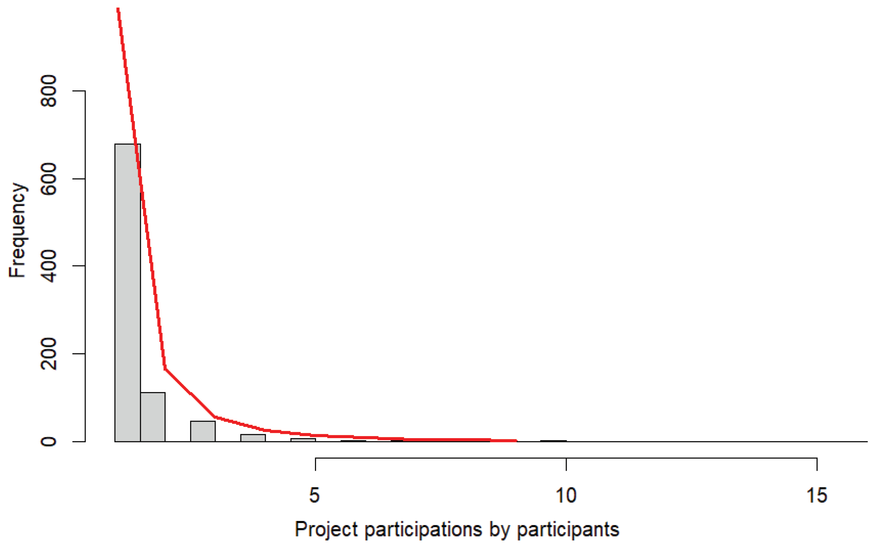
Figure 6, which depicts the frequency of project participations by participants, appears to support this relationship. The goodness-of-fit (power distribution) test on these values produced the results: α = 2.66 (~γ), x_min = 1, p = 1.

While the distribution of degree numbers did not follow a power function distribution, the frequency of project participations fit the initial value almost perfectly. In other words, the frequency of project participations is affected by scale-freedom, which is now recognized as an important phenomenon in scientific analyses. (It is important to note that α is slightly lower than 3.)

The network has a diameter of 6. The network diameter's standard deviation is σ = 0.76. As a result, the relationship in equation (7) is not satisfied: 6 ≉ 2 (6 ± 0.76 ≉ 2). Even though the average diameter is only 2.74, equation (8) is not clearly satisfied: 2.74 ≉ 2 (2.74 ± 0.76 ≉ 2). However, the latter result does not completely rule out the small-world.

Based on the values listed above, the network of forestry projects cannot be considered small-world or limited in scope. To be considered small-world, more network connections would be required. However, this does not rule out the possibility of a small-scale network of contacts outside of the projects. Rather, it is more likely that small and/or non-knowledge intensive forestry actors are simply under-represented in the sample due to the average number of participants per project, barriers to entry, and the attraction to those with extensive networks, and that not all contacts are recorded as project contacts. From the standpoint of forestry, the network is inherently fragmented. It houses the elites. The question is who, from the standpoint of network research, plays the decisive role in this network, and how far this intersects with the findings of other studies.

Table 1 lists the five most important project participants by degree numbers, and Table 2 by betweenness ranking.

The two tables have a significant overlap. However, to find the true relationship, it is worth calculating a rank correlation between degree and betweenness vale. Table 3 shows the values and evaluations of the different (Kendall, Pearson, Spearman) correlation coefficients. Due to the lack of normality, the Spearman correlation coefficient seems to be the most reliable.

According to Table 3, the relationship between the two variables is medium-large measured with different methods.

4. Discussion

The network of forestry project participants is neither random nor scale-free. The distribution of project participation by project participants, on the other hand, clearly shows a power distribution, i.e., the distribution is scale-free. Meanwhile, the project network is not clearly a small-world, i.e. the forestry sector lacks a sufficiently strong project network of connections.

Based on the direct results, it is reasonable to assume that the real network beyond the forestry projects may have scale-free properties, implying that there is almost certainly a knowledge-intensive, vibrant network of connections at the heart of forestry research, one that is much more central than the project network would imply. Unfortunately, in addition to the center, there are many peripheral players. There are many more of these than appear in the network of forestry projects. Furthermore, the nature of the projects makes some participants less marginal. Those involved in a small number of projects but with many participants.

Participation in these networks is an important goal for everyone involved in forestry. However, as we have seen, these networks presumably describe the area's elite. Barriers to entry into these networks will remain, and the competitive advantage of entities with international project experience will grow, both in terms of winning R&D funding and at the technological level.

A wise strategy for those outside the elite club would be to collaborate with participants in international forestry projects, not primarily to obtain EU funding, but to mutually exploit scientific, technological, and commercial benefits. Potential actors with emerging knowledge-intensive activities may, of course, seek to join forestry projects during the next funding period, but they will face a difficult challenge.

The key question for those with project experience is how far they can expand on the research and technological development carried out with EU funds to collaborate with others for mutual benefits.

Author Contributions

Conceptualization, Z.T. and A.N.; methodology, Z.T.; software, Z.T.; validation, A.N.; formal analysis, Z.T. and Z.P; investigation, A.N.; resources, A.N.; data curation, Z.T.; writing—original draft preparation, Z.T.; writing—review and editing, A.N.; visualization, Z.T.; supervision, A.N. and Z.P.; project administration, A.N.; funding acquisition, A.N. All authors have read and agreed to the published version of the manuscript.

Funding

Project no. TKP2021-NKTA-43 has been implemented with the support provided by the Ministry of Innovation and Technology of Hungary from the National Research, Development and Innovation Fund, financed under the TKP2021-NKTA funding scheme.

Data Availability Statement

The data presented in this study are available on request from the corresponding author.

Conflicts of Interest

The authors declare no conflict of interest.

References

Barabási:, A.L. Behálózva – a hálózatok új tudománya [Connected – the new science of networks.], 1st ed.; Magyar Könyvklub: Budapest, Hungary, 2003. [Google Scholar]
Barabási, A.L. Network science, 1st ed.; Cambridge University Press: Cambridge, UK, 2018. [Google Scholar]
Erdős, P.; Rényi, A. On the Evolution of Random Graphs. Magyar Tud. Akad. Mat. Kutató Int. Közl. 1960, 5, 17–61. [Google Scholar]
Bollobás, B. A probabilistic proof of an asymptotic formula for the number of labelled regular graphs. European J. Combin. 1980, 4, 311–316. [Google Scholar] [CrossRef]
Molloy, M.; Reed, B. Critical point for random graphs with a given degree sequence. Random Structures & Algorithms 1995, 2-3, 161–180. [Google Scholar] [CrossRef]
Newmann, M.E. Networks: An Introduction, 1st ed.; Oxford University Press: Oxford, UK, 2010. [Google Scholar]
Watts, D.J.; Strogatz, S.H. Collective dynamics of ‘small-world’ networks. Nature 1998, 393, 440–442. [Google Scholar] [CrossRef] [PubMed]
Barabási, A.L.; Albert, R. Emergence of scaling in random networks. Science 1999, 286, 509–512. [Google Scholar] [CrossRef] [PubMed]
Molnár, L. A hálózatelemzés alapfogalmai – gráfok, centralitás, szomszédosság, hidak és a kis világ. [Basic concepts of network analysis – graphs, centrality, adjacency, bridges and the small world.] In Rendszerelmélet [Systems theory]; Sasvári, P., Ed.; Dialóg Campus: Budapest, Hungary, 2020; pp. 123–140. [Google Scholar] [CrossRef]
Kisfalusi, D. Az exponenciális random gráf modellek bemutatása: Egy iskolai osztály baráti hálózatának modellezése. [Demonstration of exponential random graph models: modelling the friendship network of a school class.] Szociológiai Szemle 2018, 2, 75–88. [Google Scholar] [CrossRef]
Barabási, A.L. A hálózatok tudománya [The science of networks], 1st ed.; Libri: Budapest, Hungary, 2017. [Google Scholar]
Acock, A.C. A Gentle Introduction to Stata, 6th ed.; Stata Press: Lakeway Drive, United States, 2018. [Google Scholar]
IBM Corp. IBM SPSS Advanced Statistics, 27th ed.; IBM Corp.: Armonk, United States, 2020. [Google Scholar]
Delignette-Muller, M.L.; Dutang, C. fitdistrplus: An R Package for Fitting Distributions, 1st ed.; R Foundation: Vienna, Austria, 2020. [Google Scholar]
Clauset, A.; Shalizi, C.R.; Newman, M.E. Power-law distributions in empirical data. SIAM Review 2009, 4, 661–703. [Google Scholar] [CrossRef]
Gillespie, C.S. The poweRlaw package: Examples, 1st ed.; R Foundation: Vienna, Austria, 2020. [Google Scholar]
Cullen, A.; Frey, H. Probabilistic Techniques in Exposure Assessment, 1st ed.; Springer: New York, United States, 1999. [Google Scholar]
Efron, B.; Tibshirani, R. An Introduction to the Bootstrap, 1st ed.; Chapman and Hall/CRC: London, United Kingdom, 1994. [Google Scholar]
Barabási, A.L. A hálózatok tudománya: a társadalomtól a webig. [The science of networks: from society to the web.] Magyar Tudomány 2006, 11, 1298–1308. [Google Scholar]
Kürtösi, Z. A társadalmi kapcsolatháló-elemzés módszertani alapjai. [Methodological foundations of social network analysis.] In Társadalmi kapcsolathálózatok elemzése. [Social network analysis.], 1st ed.; Takács, K., Ed.; BCE Szociológia és Társadalompolitika Intézet: Budapest, Hungary, 2011; pp. 19–31. [Google Scholar]
Freeman, L.C. A Set of Measures of Centrality Based on Betweenness. Sociometry 1977, 1, 35–41. [Google Scholar] [CrossRef]

Figure 1. Project participants' network.

Figure 2. Degree frequencies.

Figure 3. Degrees-based rootogram.

Figure 4. Cullen and Frey graph (discrete variable).

Figure 5. Cullen and Frey graph (continuous variable).

Figure 6. Frequency of project participations.

Table 1. Central participants by degree.

Name	Country	Degree
Luonnonvarakeskus	Finland	329
INRAE	France	217
EFI	international (in Finland)	212
CNR	Italy	182
Nibio	Norway	182

Table 2. Central participants by betweenness.

Name	Country	Betweenness
Luonnonvarakeskus	Finland	61868.45
INRAE	France	29427.73
Fraunhofer-Gesellschaft	Germany	28593.36
CREA	Italy	23422.10
CNR	Italy	18864.35

Table 3. Correlation coefficients.

Method	Value	Relationship
Kendall	τ = 0.46 (p = 0)	medium
Pearson	r = 0.75 (p = 0)	large
Spearman	ρ = 0.56 (p = 0)	large

Disclaimer/Publisher’s Note: The statements, opinions and data contained in all publications are solely those of the individual author(s) and contributor(s) and not of MDPI and/or the editor(s). MDPI and/or the editor(s) disclaim responsibility for any injury to people or property resulting from any ideas, methods, instructions or products referred to in the content.

© 2023 by the authors. Licensee MDPI, Basel, Switzerland. This article is an open access article distributed under the terms and conditions of the Creative Commons Attribution (CC BY) license (http://creativecommons.org/licenses/by/4.0/).

Copyright: This open access article is published under a Creative Commons CC BY 4.0 license, which permit the free download, distribution, and reuse, provided that the author and preprint are cited in any reuse.

MDPI Initiatives

Important Links

Choose an area of interest and we will send you notifications of new preprints at your preferred frequency.

Disclaimer

Social Network Analysis in Forestry Projects

Abstract

1. Introduction

2. Materials and Methods

3. Results

3.1. Creating the network of connections

3.2. Calculated network indicator values and fit test results

4. Discussion

Author Contributions

Funding

Data Availability Statement

Conflicts of Interest

References

MDPI Initiatives

Important Links

Subscribe