Submitted:
11 May 2023
Posted:
12 May 2023
You are already at the latest version
Abstract
Keywords:
1. Introduction
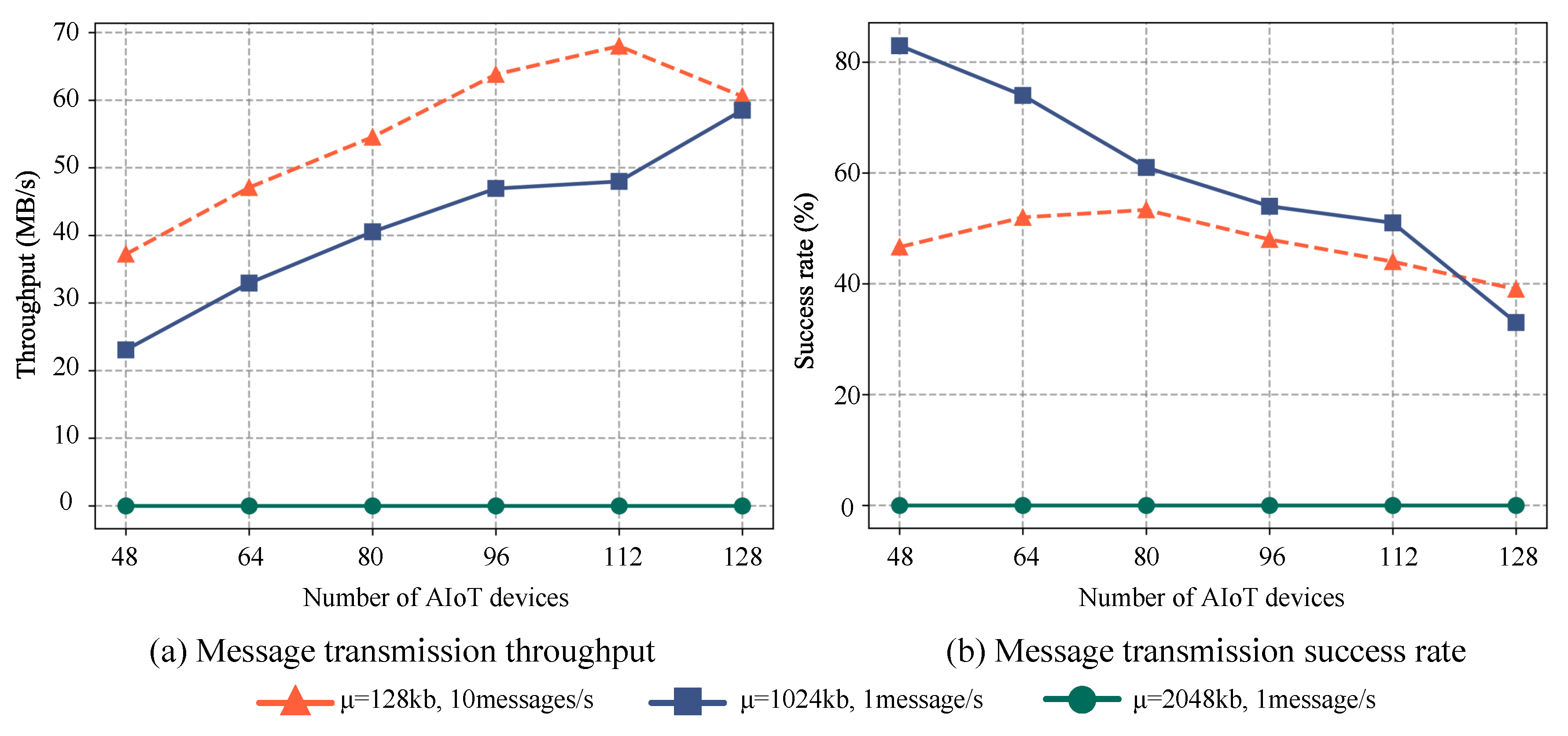
- We investigate the potential factors that affect system performance in a high-demand, large-scale messaging scenario using an existing distributed message queue system. To address this issue, we propose a partition selection algorithm for distributed message queues that enhances system throughput and improves message delivery success rates with appropriate configurations. We conduct evaluations to demonstrate the necessity of optimizing configurations for improved transmission performance in highly concurrent messaging scenarios at a large scale.
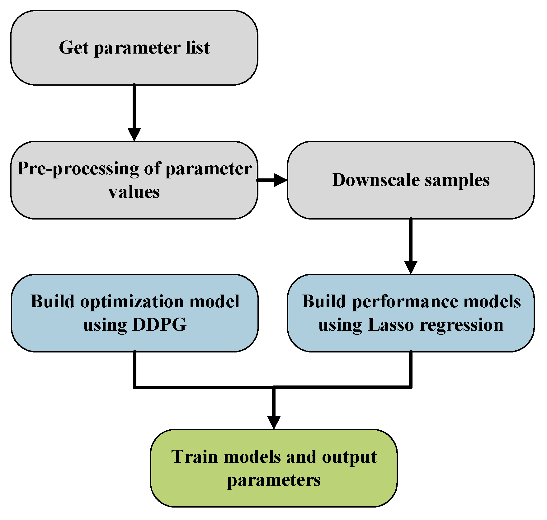
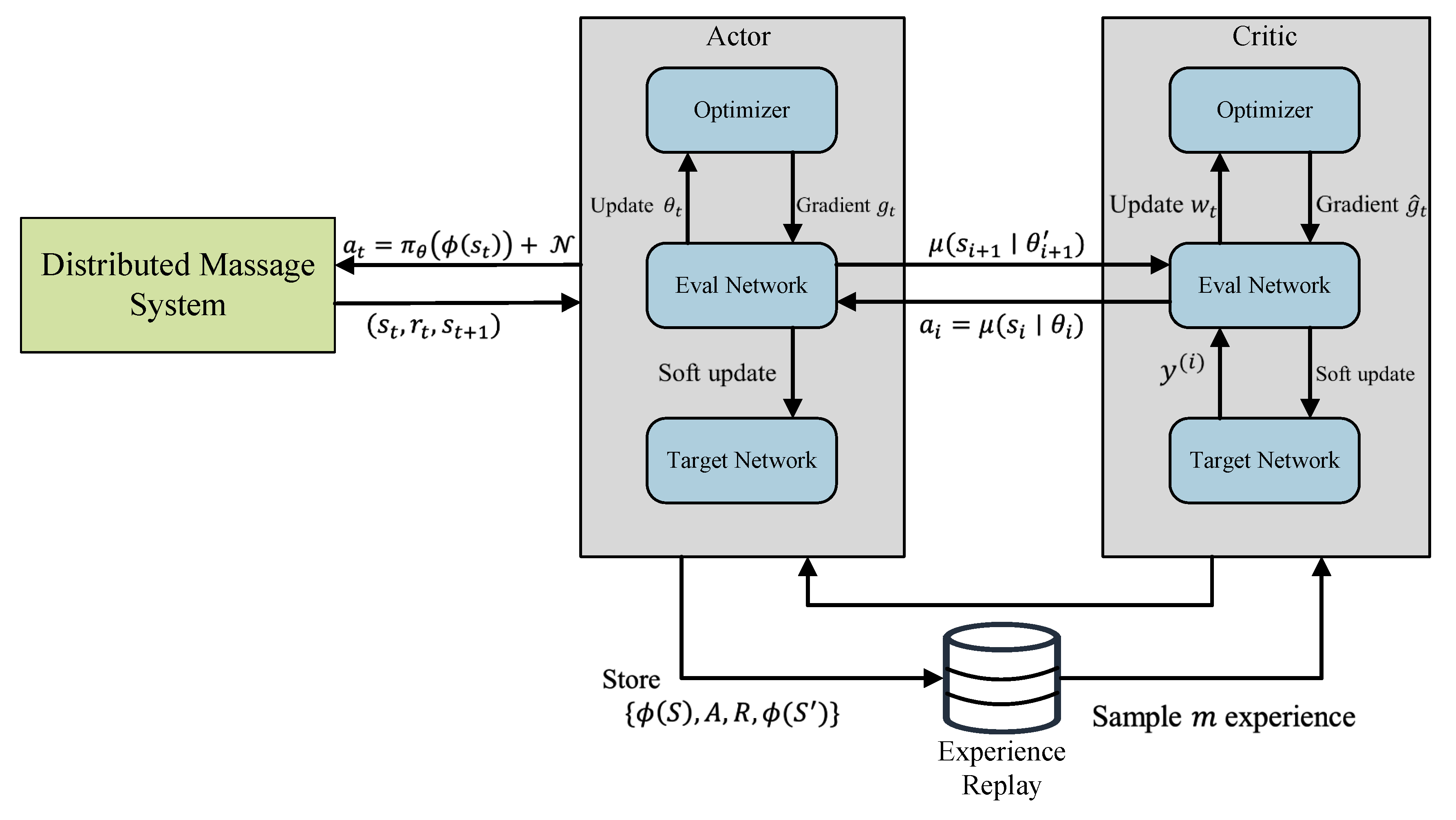
- We propose a DDPG-based Distributed Message Queue Systems Configuration Optimization algorithm (DMSCO), which leverages a pre-processed parameter list as an action space to train a decision model. By constructing rewards based on the distributed message queue system’s throughput and message transmission success rate, the DMSCO algorithm can effectively optimize messaging performance in various AIoT scenarios by adapting the optimal parameter configurations.
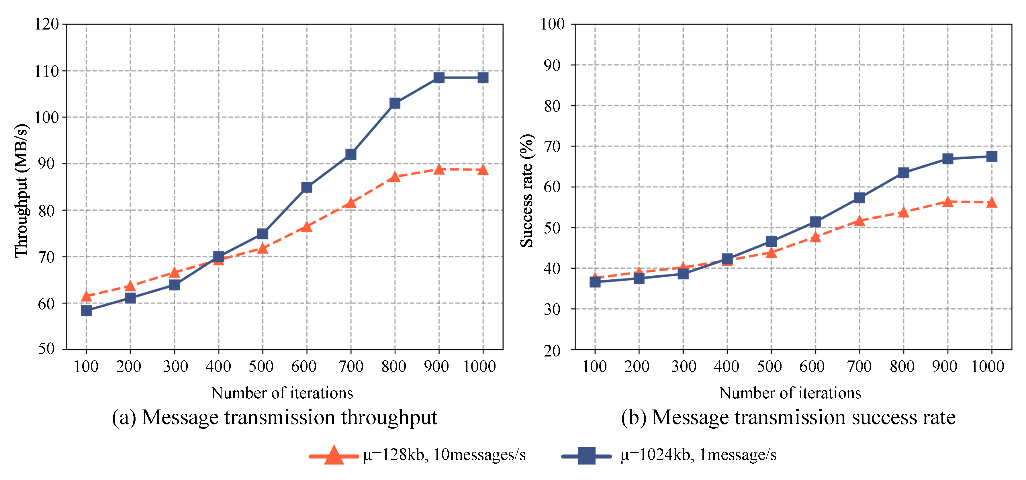
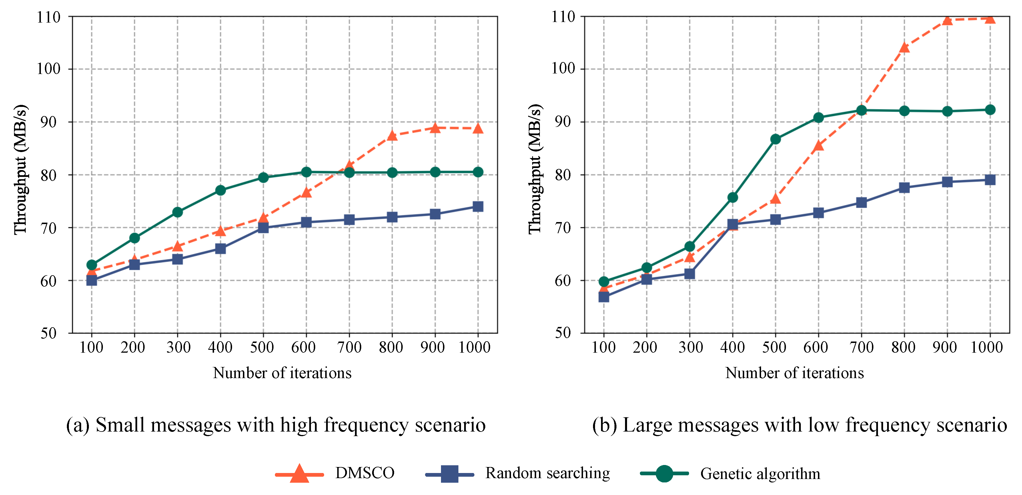
- We evaluated the proposed DMSCO algorithm under varying message sizes and transmission frequency cases to validate its performance efficacy for the distributed message queue system in different AIoT Edge computing scenarios. Our comparative analysis against methods utilizing genetic algorithms and random searching revealed that the proposed DMSCO algorithm offers an efficient solution to address the unique demands of larger-scale, high-concurrency AIoT Edge computing applications.
2. Related Work
3. Distributed Message Queue System for AIoT Edge Computing
3.1. Distributed message system for Large-scale Message Transmission Scenarios
- Administrator module: this module assumes responsibility for the management and upkeep of all information associated with Topics and Partitions.
- API module: this module assumes the crucial role of encoding, decoding, assembling, and facilitating interactions with data.
- Client module: this module carries the responsibility of retrieving Broker metadata from Zookeeper and acquiring essential information regarding the mapping of Topics and Partitions.
- Cluster module: this module encompasses a collection of classes and their corresponding descriptions for key components such as Broker, cluster, partition, and replica.
- Control module: This module assumes a crucial role in overseeing various tasks, including leader election, replica allocation, partition expansion, and replica expansion.
| Algorithm 1: Partition selection algorithm |
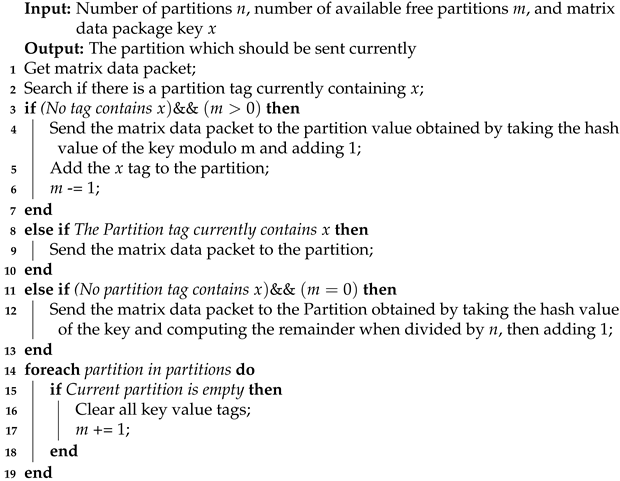 |
3.2. Performance modeling in Large-Scale Scenarios
4. Reinforcement Learning-based Method for Optimized AIoT Message Queue System
4.1. Parameter Screening
| Algorithm 2: Dimensionality reduction method based on PCA for the initial training sample set |
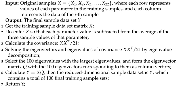 |
4.2. Lasso regression-based performance modeling
| Algorithm 3: Key parameter screening method based on Lasso regression |
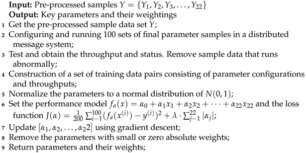 |
4.3. Parameter optimization method based on deep deterministic policy gradient algorithm
| Algorithm 4: DDPG based distributed message system configuration optimization (DMSCO) |
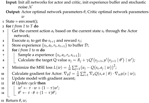 |
5. Experiments
5.1. Comparison set up
5.2. Analysis on performance and results
6. Conclusions
Author Contributions
Funding
Institutional Review Board Statement
Informed Consent Statement
Data Availability Statement
Conflicts of Interest
References
- Peres, R.S.; Jia, X.; Lee, J.; Sun, K.; Colombo, A.W.; Barata, J. Industrial artificial intelligence in industry 4.0-systematic review, challenges and outlook. IEEE Access 2020, 8, 220121–220139. [Google Scholar] [CrossRef]
- Ullah, Z.; Al-Turjman, F.; Mostarda, L.; Gagliardi, R. Applications of artificial intelligence and machine learning in smart cities. Computer Communications 2020, 154, 313–323. [Google Scholar] [CrossRef]
- Li, H.; Ota, K.; Dong, M. Learning IoT in edge: Deep learning for the Internet of Things with edge computing. IEEE Network 2018, 32, 96–101. [Google Scholar] [CrossRef]
- de Freitas, M.P.; Piai, V.A.; Farias, R.H.; Fernandes, A.M.R.; de Moraes Rossetto, A.G.; Leithardt, V.R.Q. Artificial Intelligence of Things Applied to Assistive Technology: A Systematic Literature Review. Sensors 2022, 22. [Google Scholar] [CrossRef] [PubMed]
- Bourechak, A.; Zedadra, O.; Kouahla, M.N.; Guerrieri, A.; Seridi, H.; Fortino, G. At the Confluence of Artificial Intelligence and Edge Computing in IoT-Based Applications: A Review and New Perspectives. Sensors 2023, 23. [Google Scholar] [CrossRef] [PubMed]
- Ionescu, V.M. The analysis of the performance of RabbitMQ and ActiveMQ. In Proceedings of the 14th RoEduNet International Conference-Networking in Education and Research (RoEduNet NER). IEEE, 2015, pp. 132–137.
- Yue, M.; Ruiyang, Y.; Jianwei, S.; Kaifeng, Y. A MQTT protocol message push server based on RocketMQ. In Proceedings of the 2017 10th International Conference on Intelligent Computation Technology and Automation (ICICTA). IEEE, 2017, pp. 295–298.
- Snyder, B.; Bosanac, D.; Davies, R. Introduction to apache activemq. Active MQ in action 2017, pp. 6–16.
- Wu, H.; Shang, Z.; Wolter, K. Performance Prediction for the Apache Kafka Messaging System. In Proceedings of the 21st IEEE International Conference on High Performance Computing and Communications, 2019, pp. 154–161.
- Jo, H.C.; Jin, H.W.; Kim, J. Self-adaptive end-to-end resource management for real-time monitoring in cyber-physical systems. Computer Networks 2023, 225, 109669. [Google Scholar] [CrossRef]
- Stewart, J.C.; Davis, G.A.; Igoche, D.A. AI, IoT, and AIoT: Definitions and impacts on the artificial intelligence curriculum. Issues in Information Systems 2020, 21. [Google Scholar]
- Le Noac’H, P.; Costan, A.; Bougé, L. A performance evaluation of Apache Kafka in support of big data streaming applications. In Proceedings of the 2017 IEEE International Conference on Big Data (Big Data). IEEE, 2017, pp. 4803–4806.
- Nguyen, C.N.; Hwang, S.; Kim, J.S. Making a case for the on-demand multiple distributed message queue system in a Hadoop cluster. Cluster Computing 2017, 20, 2095–2106. [Google Scholar] [CrossRef]
- Dong, W.; Woźniak, M.; Wu, J.; Li, W.; Bai, Z. Denoising aggregation of graph neural networks by using principal component analysis. IEEE Transactions on Industrial Informatics 2022, 19, 2385–2394. [Google Scholar] [CrossRef]
- Sarker, I.H. Machine learning: Algorithms, real-world applications and research directions. SN computer science 2021, 2, 160. [Google Scholar] [CrossRef] [PubMed]
- Fu, G.; Zhang, Y.; Yu, G. A fair comparison of message queuing systems. IEEE Access 2020, 9, 421–432. [Google Scholar] [CrossRef]
- Bao, L.; Liu, X.; Xu, Z.; Fang, B. Autoconfig: Automatic configuration tuning for distributed message systems. In Proceedings of the 33rd ACM/IEEE International Conference on Automated Software Engineering, 2018, pp. 29–40.
- Shakya, S.; et al. IoT based F-RAN architecture using cloud and edge detection system. Journal of ISMAC 2021, 3, 31–39. [Google Scholar] [CrossRef]
- Brünink, M.; Rosenblum, D.S. Mining performance specifications. In Proceedings of the ACM SIGSOFT International Symposium on Foundations of Software Engineering, FSE. ACM, 2016, pp. 39–49.
- Grochla, K.; Nowak, M.; Pecka, P.; et al. Influence of Message-Oriented Middleware on Performance of Network Management System: A Modelling Study. In Proceedings of the Multimedia and Network Information Systems - Proceedings of the 10th International Conference MISSI, 2016, Vol. 506, Advances in Intelligent Systems and Computing, pp. 379–393.
- Henard, C.; Papadakis, M.; Harman, M.; Le Traon, Y. Combining multi-objective search and constraint solving for configuring large software product lines. In Proceedings of the 2015 IEEE/ACM 37th IEEE International Conference on Software Engineering. IEEE, 2015, Vol. 1, pp. 517–528.
- He, H.; Jia, Z.; Li, S.; Yu, Y.; Zhou, C.; Liao, Q.; Wang, J.; Liao, X. Multi-Intention-Aware Configuration Selection for Performance 550 Tuning. In Proceedings of the 44th International Conference on Software Engineering, New York, NY, USA, 2022; ICSE ’22, p. 551 1431–1442. [CrossRef]
- Sarkar, A.; Guo, J.; Siegmund, N.; Apel, S.; Czarnecki, K. Cost-efficient sampling for performance prediction of configurable systems (t). In Proceedings of the 2015 30th IEEE/ACM International Conference on Automated Software Engineering (ASE). IEEE, 2015, pp. 342–352.
- Tao, Z.; Xia, Q.; Hao, Z.; Li, C.; Ma, L.; Yi, S.; Li, Q. A survey of virtual machine management in edge computing. Proceedings of the IEEE 2019, 107, 1482–1499. [Google Scholar] [CrossRef]
- Gou, F.; Wu, J. Message transmission strategy based on recurrent neural network and attention mechanism in IoT system. Journal of Circuits, Systems and Computers 2022, 31, 2250126. [Google Scholar] [CrossRef]
- Fu, G.; Zhang, Y.; Yu, G. A Fair Comparison of Message Queuing Systems. IEEE Access 2021, 9, 421–432. [Google Scholar] [CrossRef]
- Wang, Y.; Xiang, Z.J.; Ramadge, P.J. Lasso screening with a small regularization parameter. In Proceedings of the IEEE 561 International Conference on Acoustics, Speech and Signal Processing, ICASSP. IEEE, 2013, pp. 3342–3346.
- Lillicrap, T.P.; Hunt, J.J.; Pritzel, A.; Heess, N.; et al. Continuous control with deep reinforcement learning. In Proceedings of the 4th International Conference on Learning Representations, ICLR, 2016.
- Johnson, J.M.; Khoshgoftaar, T.M. Encoding high-dimensional procedure codes for healthcare fraud detection. SN Computer Science 2022, 3, 362. [Google Scholar] [CrossRef]
| Parameter name | weight |
|---|---|
| bThreads | 15.03 |
| cType | 70.35 |
| nNThreads | 23.74 |
| nIThreads | 25.16 |
| mMBytes | 60.35 |
| qM·Requests | 124.32 |
| nRFetchers | -24.59 |
| sRBBytes | 70.42 |
| sSBBytes | 120.35 |
| sRMBytes | 54.36 |
| acks | 43.58 |
| bMemory | 73.66 |
| bSize | -170.95 |
| lMs | 34.32 |
Disclaimer/Publisher’s Note: The statements, opinions and data contained in all publications are solely those of the individual author(s) and contributor(s) and not of MDPI and/or the editor(s). MDPI and/or the editor(s) disclaim responsibility for any injury to people or property resulting from any ideas, methods, instructions or products referred to in the content. |
© 2023 by the authors. Licensee MDPI, Basel, Switzerland. This article is an open access article distributed under the terms and conditions of the Creative Commons Attribution (CC BY) license (http://creativecommons.org/licenses/by/4.0/).


