Assessment of Aerodynamic Plates Subjected to Von Kármán Vortex Street for Enhancing the Wind Energy Generation in Blade-less Devices

This study explores the feasibility of using an oscillating plate downstream of a cylindrical body to produce mechanical energy from a Von Kármán vortex street. The study aims to quantify the impact of the plate length, its separation from the cylinder, and a machine damping factor on the power coefficient and the blade’s displacement to identify the optimal configuration. This preliminary assessment assumes that the plate oscillation is small enough to avoid changes in the vortex dynamics. This assumption allows the construction of a surrogate model using CFD to evaluate the effect of plate length and separation from the cylinder on the fluctuating lift forces over the plate. Later, the surrogate model, combined with varying machine damping factors, facilitates the description of the device’s dynamics through the numerical integration of an angular momentum equation. The results showed that a plate with 0.52D length, 5.548D separation from the cylinder, and a damping factor of 0.013 achieved a power coefficient of 0.147 and a perpendicular displacement of 0.266D. These results demonstrate a substantial improvement in the performance of bladeless generators.

Keywords:

Subject: Engineering - Energy and Fuel Technology

1. Introduction

Wind generators are machines commonly implemented to transform the kinetic energy of wind into electricity through sustainable and efficient processes. Among available technology in the field, horizontal devices are popular due to their high-power coefficient (able to transform more than 40% of the wind kinetic energy). Therefore, this type of generator prompts feeding twelve per cent of the electrical energy consumption worldwide, contributing to over 1100 GW by 2020 [1].

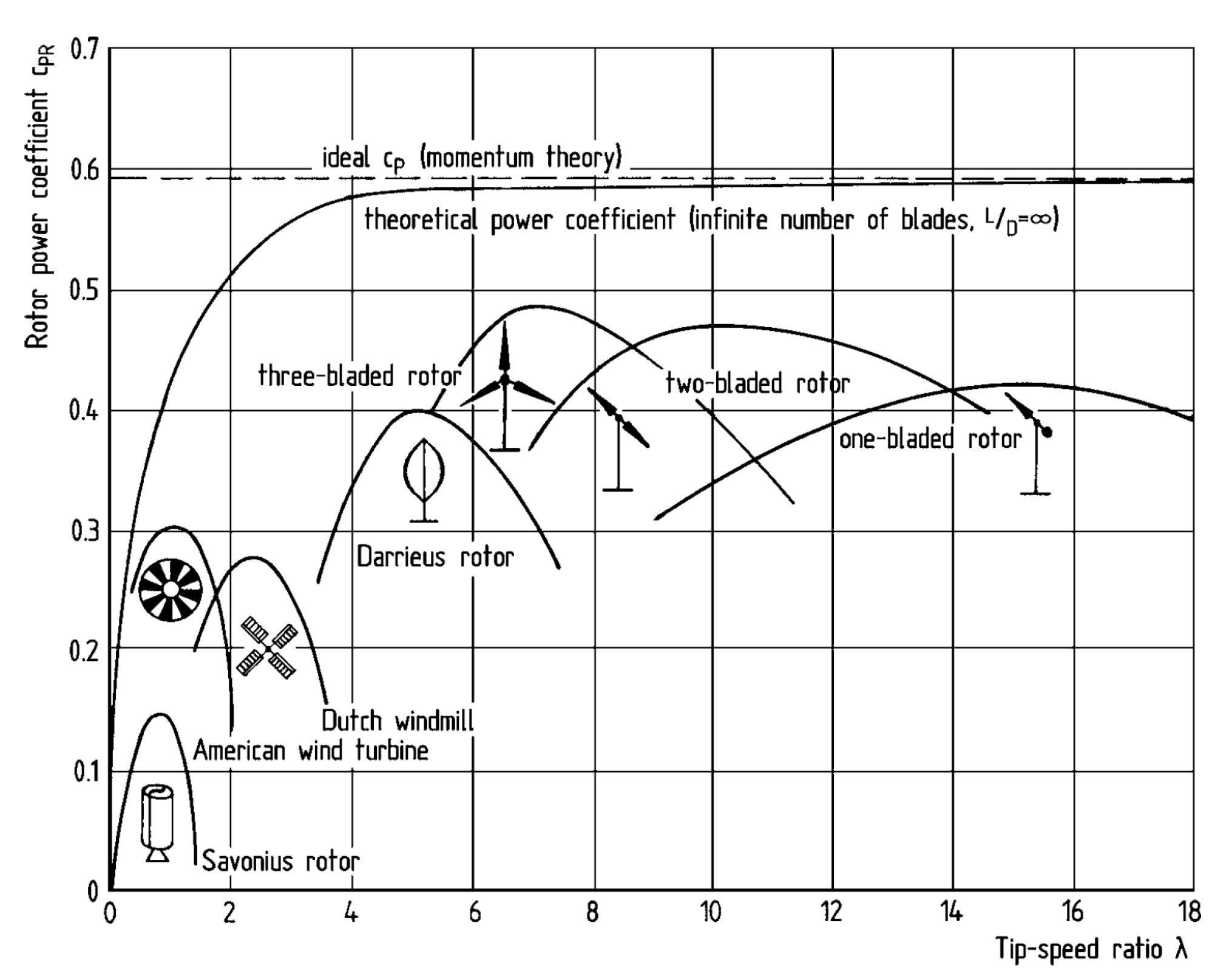
Although horizontal wind turbines have a high-power coefficient, researchers and manufacturers are also exploring small-generation wind turbines to produce electricity in remote regions. This scenario presents new challenges, such as size reduction, low complexity in manufacturing, low maintenance costs and low noise. Figure 1 shows some of these options, including the Savonius turbine and the Darrieus turbine, which are vertical-axis wind turbines.

According to Figure 1, it is easy to state that the energy extraction from wind mainly comes from devices that transform mechanical energy into rotating shaft work. However, novel options that convert kinetic energy into oscillating work are gaining interest in the scientific community. These apparatuses are commonly known as bladeless generators [3].

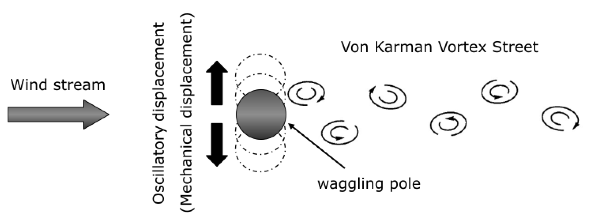
Figure 2 illustrates a schematic depiction of bladeless generators, characterised by cylindrical or conical poles that generate a Von Kármán vortex street when wind passes over them. The Von Kármán vortexes have the potential to produce vibrations in these poles through an aero-elastic resonance of its structure, transformed, later on, into electricity by implementing magnetic induction generators [3].

Different experiments and CFD analyses have addressed the study of these types of machines; for example, the work of [4,5,6,7,8,9,10]. Moreover, [3] launched, onto the market, two commercial devices known as Vortex Nano and Vortex Tacoma. According to [11], Nano can generate 0.9W of power when a prototype 0.85 m in height is 8 m above ground level, exposed to a wind speed of 6.5 m/s, while Tacoma can generate 110 W with wind speed of 9 m/s. [11] also projected that a generator with a height of 2.75 m could transform 30% of the wind energy into electrical work, which represents an appropriate increment in conversion efficiency.

Apart from the design of [3], some researchers have studied configurations that included bulk or aerodynamic shapes at the rear of a rigid pole to exploit the vortex energy at the wake zone. For example, [12] studied the aerodynamic behaviour of three bodies exposed to a Reynolds number of 100, demonstrating that vortexes can produce work in a stable process according to the dimension of the bodies. In addition, [13] simulated the alterations in the vortexes’ dynamic of a flow with low Reynolds Numbers (Laminar condition) produced by different plates set downstream on the pole. Finally, [14] studied the behaviour of aerodynamic surfaces in a test bench that could alter the distance of these surfaces from a cylindrical pole and their stiffness. This experiment reported an optimal separation of three to four times the cylinder diameter for a fluid with a Reynolds Number between 100 and 200, as this assures an appropriate development of vortexes, able to interact fully with the plate.

The present work aims to study the impact of Von Kármán vortex street on a plate downstream of a rigid cylinder (pole) to harness vortex energy in the wake zone. The study employs a multi-objective optimisation approach to determine the plate length and distance from the cylinder that maximises the power coefficient of the device while minimising its oscillation amplitude. The plate length varies between 0.5D and 1D, while the cylinder-plate separation ranges from 1D to 7D. The evaluation considers a Reynolds number of 72,500, as [15] reported high values of lift coefficient on bladeless devices at this condition.

2. The Studied Problem: Device’s Structural Dynamics Responses

The studied wind-generator concept involves a plate with a single degree of freedom oscillating along an axis aligned with the length of an upstream-placed cylinder. The oscillation occurs due to a fluctuating lift force on the plate, which appears when the plate is exposed to the wake generated by the cylinder on a crossing fluid. Finally, the lift force creates torque with a fluctuating angular velocity, which turns into electricity through magnetic induction. 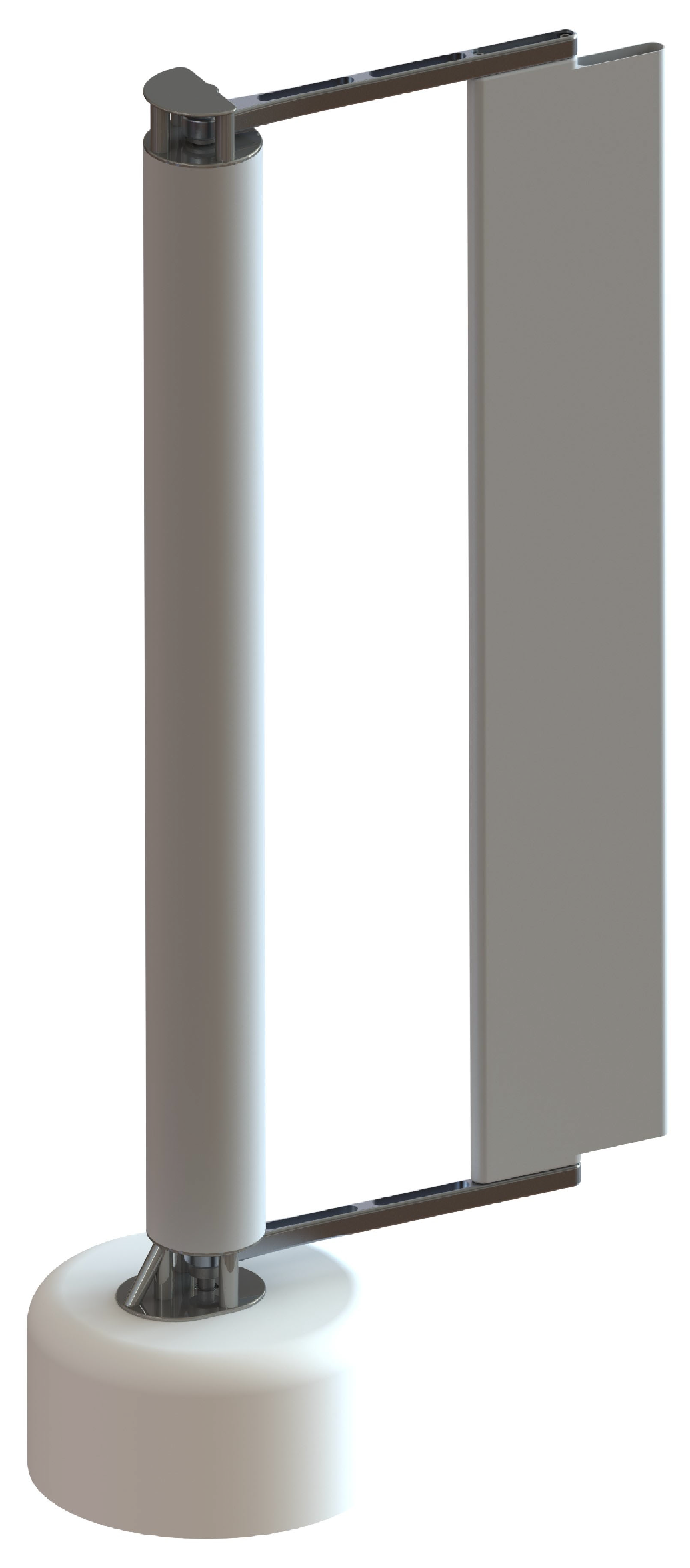Figure 3 shows a model of the whole device.

The fluctuating lift force on the bladeless plate, which favours its vibration, depends on the cylinder-plate separation (S), plate length (L) and the Von Kármán vortex street dynamics. Its study, therefore, demands either laboratory tests or the application of CFD. In addition, Newton’s second law of motion in a rotational framework governs the response of this vibrating system to external driving forces

F_{L}

, for known values of the damping factor

ξ

, restoration forces K, and the body inertia

I_{0}

[16], and this indicates that a maximum power conversion of bladeless devices occurs at their resonance conditions.

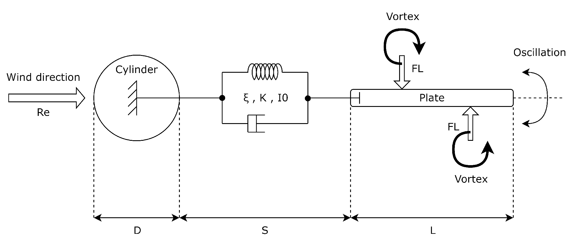
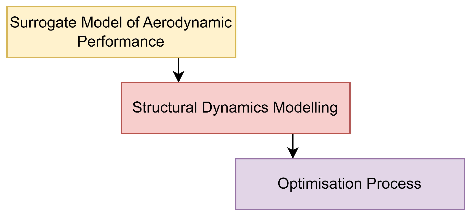
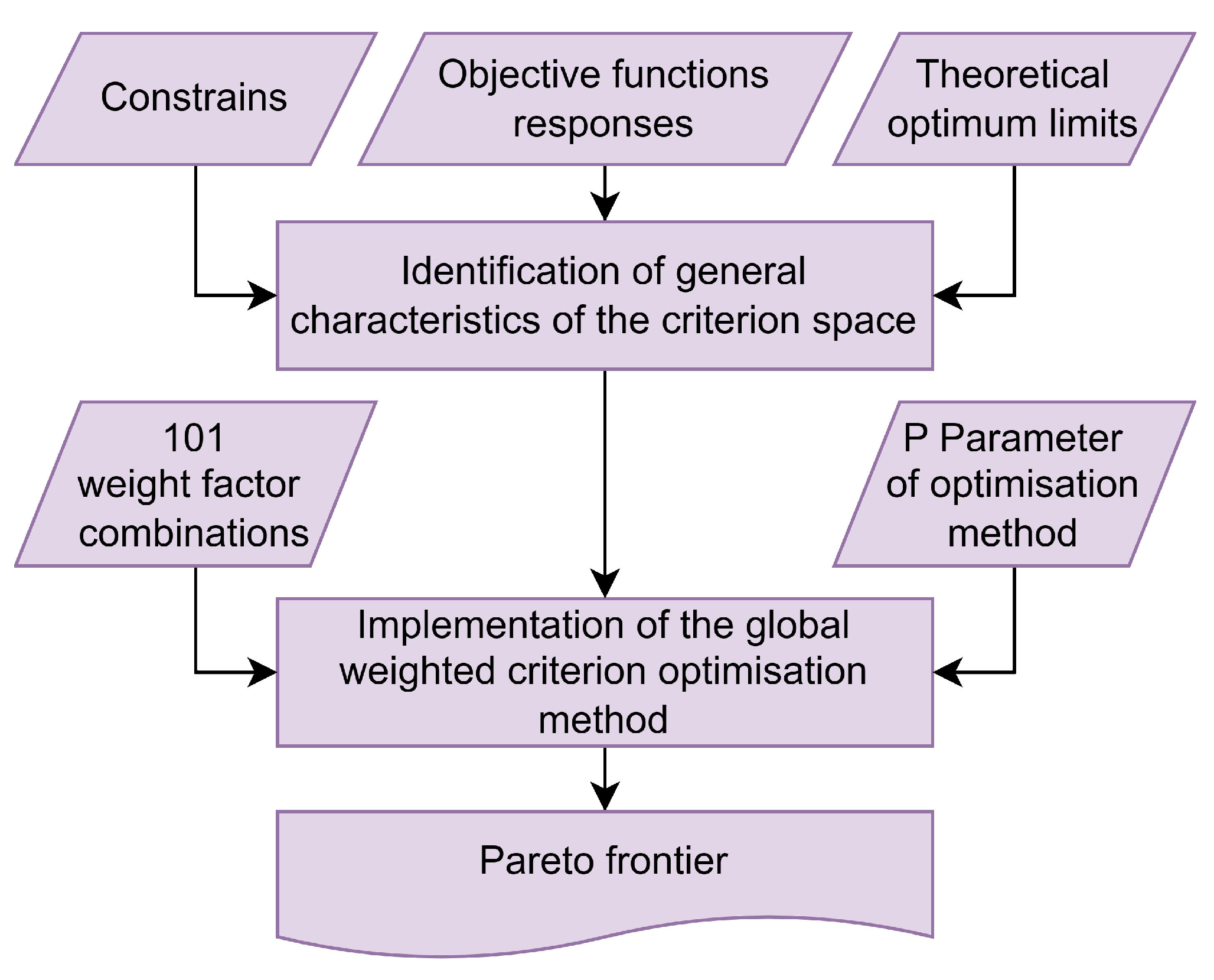
Figure 4 shows a simplified representation of the device configuration and the vortexes interaction. Figure 5, moreover, presents an overview of the plan followed by this work, which include the development of a surrogate model to account for the fluid dynamic effect, the construction of a structural-dynamic model to link variables with the objective functions, and the running of an optimisation process.

3. Methodology

3.1. Studied variables

The dynamic behaviour of the studied configuration is a function of multiple variables, which are commonly expressed as non-dimensional quantities. This work centres its attention on four of them for a fixed Reynolds Number, as follows:

3.1.1. The Lift-Coefficient

It is a non-dimensional parameter widely used in aerodynamic profiles. This value measures the ratio between the lift force (parallel to the flow direction) and a force derived from the dynamic pressure.

Equation (1) allows computing the Lift-Coefficient, where

F_{L}

is the lift force,

V_{\infty}

is the free-stream velocity magnitude,

ρ

is the fluid density, and s represents a surface area of reference. A suitable bladeless generator must assure a high RMS value of this amount.

C l = \frac{F_{L}}{\frac{1}{2} ρ {V_{\infty}}^{2} s}

(1)

When working with discrete values, such as lab measurements or transient CFD results, the non-dimensional lift coefficient expresses as a root mean square (RMS) value (

C l^{'}

) computed during a specific time interval. Eqn. (2) gives the mathematical expression of (

C l^{'}

), where i represents a discrete value of n data.

C l^{'} = \sqrt{\frac{1}{n} \sum_{i = 1}^{n} {C l_{i}}^{2}}

(2)

3.1.2. The Strouhal number

It describes the ratio between a characteristic flow time and an oscillation period. This parameter allows describing the Von Kármán vortex frequency. Eqn. (3) represents the Strouhal number, where f is the vortex shedding frequency, L is the characteristic length and V is the free-stream velocity magnitude.

S t = \frac{f L}{V}

(3)

The vortex-shedding frequency comes from a discrete form of the Fast Fourier Transform (FFT). Eqn. (4) gives the FFT discrete format implemented during the assessment, which is available in the SciPy library [17]. In this equation,

C l [n]

denotes the N-periodic signal data,

e^{- 2 π j \frac{k n}{N}}

is the primitive nth root of unity, k is the integer frequency, n is the index of a data point, and N is the total number of data points of the discrete signal. [18] presents an in-depth study of the subject.

y [k] = \sum_{n = 0}^{N - 1} C l_{[n]} e^{- 2 π j \frac{k n}{N}}

(4)

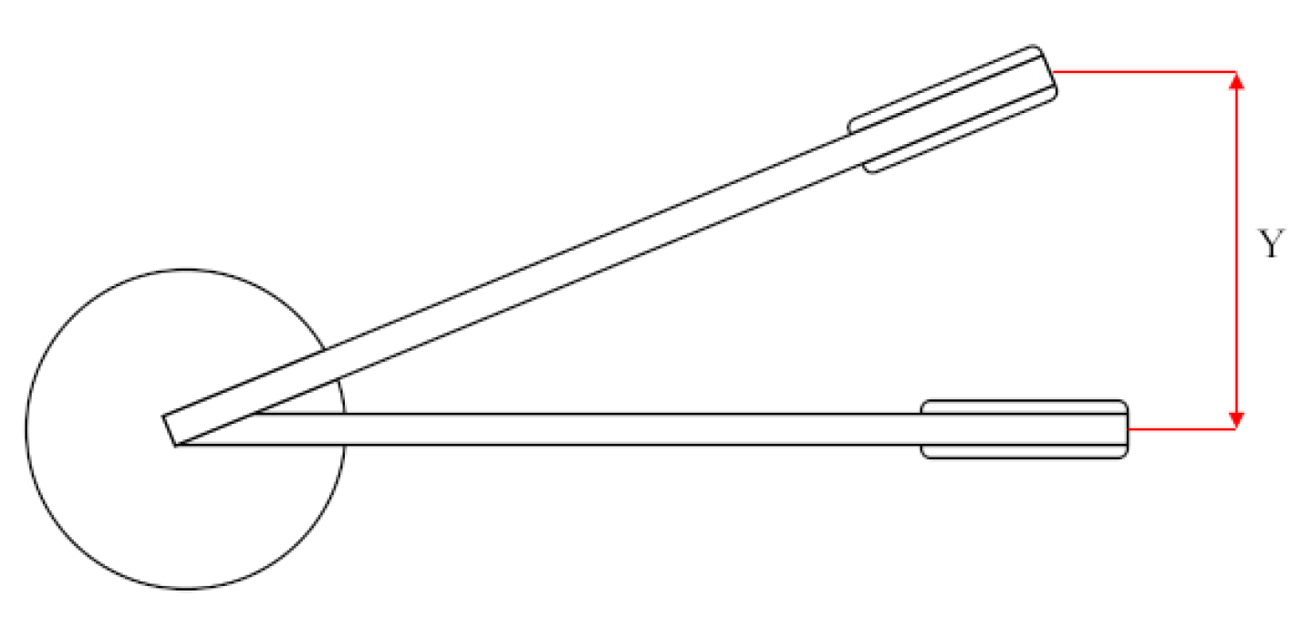
3.1.3. The perpendicular displacement

It is a dimensionless variable implemented in this study to quantify changes in the device’s relative position (in this case, the plate of the wind generator) according to its neutral position and the cylinder diameter D. Figure 6 helps describe this variable, denoted by Y.

3.1.4. The Power Coefficient

It is a non-dimensional number that allows computing the amount of power that wind generators can withdraw from the wind according to Eqn. (5). Therefore, this number emulates the conversion efficiency of a wind generator [19]:

C p = \frac{{\dot{W}}_{g e n e r a t o r}}{{\dot{W}}_{a v a i l a b l e}} = \frac{{\dot{W}}_{g e n e r a t o r}}{\frac{1}{2} ρ {V_{\infty}}^{3} A}

(5)

3.2. The Surrogate Model

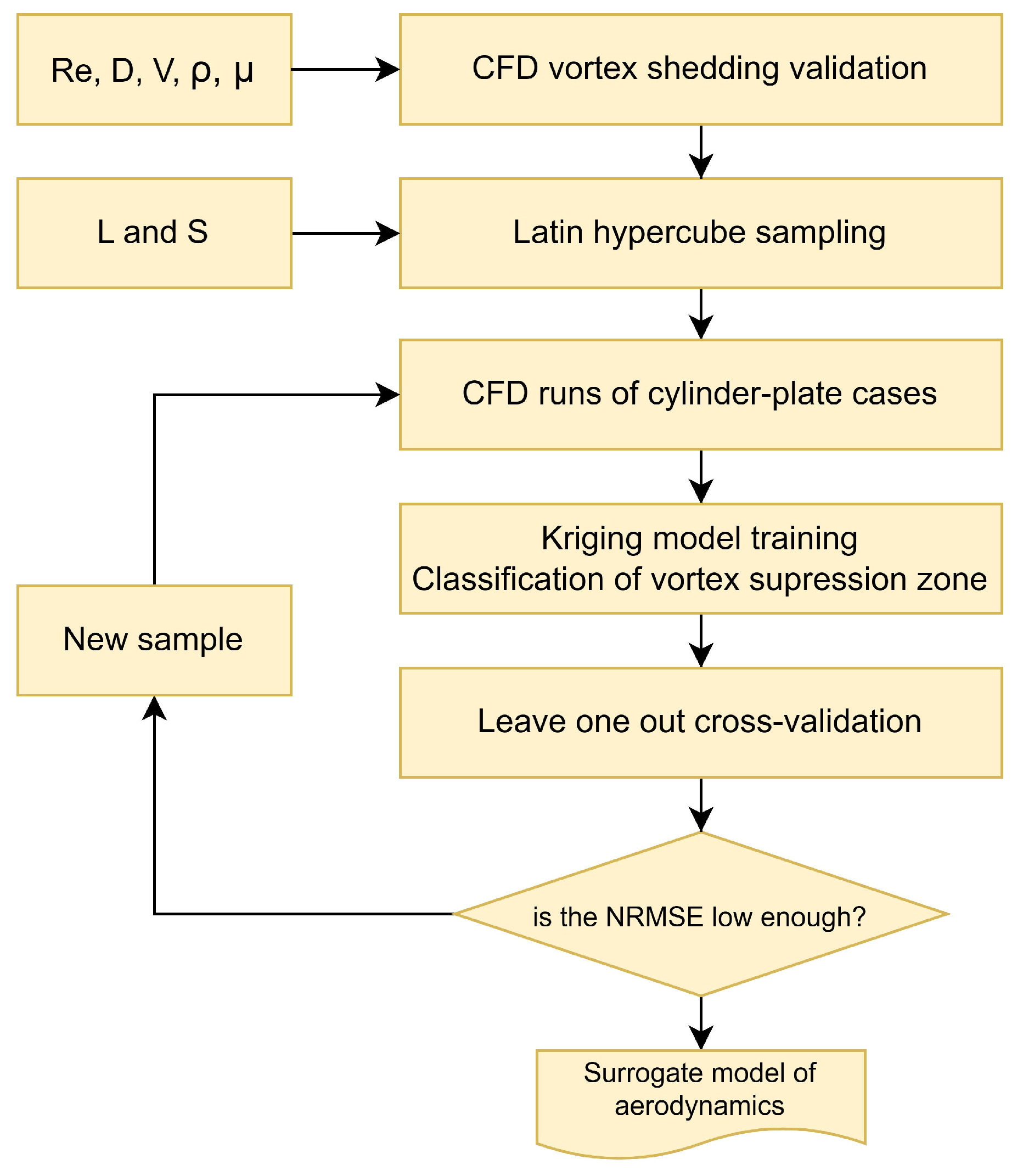
Figure 7 shows the developed methodology at this stage. Each procedure is described in the following subsections.

3.2.1. CFD model

This work implements the CFD software SimScale to compute the solution of the underlying differential equations. SimScale is a computer-aided engineering (CAE) software based on cloud computing that uses OpenFOAM at its core.

The simulation of Von Kármán’s Vortex streets requires complex turbulent models able to predict vortex oscillation according to the order of the Reynolds number set in this study. Large Eddy Simulation (LES) is a suitable option for the task because it offers accuracy with a reasonable computational cost. LES computes large eddies and their interaction, responsible for the Von Kármán Vortex dynamics while minimising the processing time by including a sub-grid filter to model small eddies.

Equation (6) represents the tensorial notation of the momentum equation of incompressible flow commonly solved by CFD codes centred on the LES model [20]. The terms on its left denote the transient behaviour of the control volume and the momentum fluxes. In addition, the ones on its right mean the contribution of any pressure gradient and the viscous stress tensor that includes the sub-grid stress tensor (

τ_{i j}

), whose aim is the artificial dissipation of eddies larger than the domain cell sizes.

\begin{matrix} ρ (\frac{\partial}{\partial t} {\underset{̲}{u}}_{i} + \frac{\partial}{\partial x_{j}} ({\underset{̲}{u}}_{i} {\underset{̲}{u}}_{j})) = \frac{\partial}{\partial x_{j}} (\frac{\partial {\underset{̲}{σ}}_{i j}}{\partial x_{i}}) \\ - \frac{\partial \underset{̲}{p}}{\partial x_{i}} - \frac{\partial {\underset{̲}{τ}}_{i j}}{\partial x_{j}} \end{matrix}

(6)

Equation (7) defines the sub-grid scale stress

{\underset{̲}{τ}}_{i j}

. This equation includes

μ_{t}

as the subgrid-scale eddy viscosity,

\underset{̲}{S_{i j}}

as the resolved scale rate of strain tensor,

{\underset{̲}{τ}}_{i j}

as the isotropic part of the sub-grid scale stresses and

{\underset{̲}{σ}}_{i j}

as the stress tensor due to molecular viscosity [20].

{\underset{̲}{τ}}_{i j} = \frac{1}{3} {\underset{̲}{τ}}_{k k} δ_{i j} - 2 μ_{t} {\underset{̲}{S}}_{i j}

(7)

Different options allow calculating

μ_{t}

. This work makes use of the Smagorinsky-Lilly model (homogeneous isotropic turbulence). On the one hand, the Smagorinsky-Lilly model is simple, easy to implement, and numerically cheap [21]. Moreover, Open FOAM includes a well developed library of this option.

Equation (8) shows the subgrid-scale eddy viscosity

μ_{t}

of to the Smagorinsky-Lilly model according to the Open FOAM documentation [20]. In this equation,

C_{s}

is the Smagorinsky coefficient, set equal to 0.094 [22],

L_{s}

represents the mixing length for sub-grid scales, and

|\underset{̲}{S}| = \sqrt{2 {\underset{̲}{S}}_{i j} {\underset{̲}{S}}_{i j}}

μ_{t} = μ_{s g s} = ρ {L_{s}}^{2} {C_{s}}^{2} |\underset{̲}{S}|

(8)

An in-depth discussion about this topic is presented by [23,24].

3.2.2. Model setup

The model setup follows the SimScale validation tutorial titled Large Eddy Simulation of Flow Over a Cylinder [25], but with changes that ensure a Reynolds number of 72500, as described in Table 1, Table 2 and Table 3.

The time step of the model changes according to the Courant number. The last one is limited to a range between

0.7

and

0.8

. Moreover, the sampling frequency to compute the RMS lift coefficient and the Strouhal number correspond to a value of 10 time steps.

3.2.3. CFD Vortex Shedding Validation

The Von Kármán Vortex Street is strongly connected to the vortex shedding on the bluff body surface. Therefore, the CFD simulation must guarantee adequate modelling of the boundary layer around that body.

Accordingly, a mesh whose resolution assures an appropriate aspect ratio of the cells near the bluff body and an adequate number of layers along any radial projection from this body is necessary. 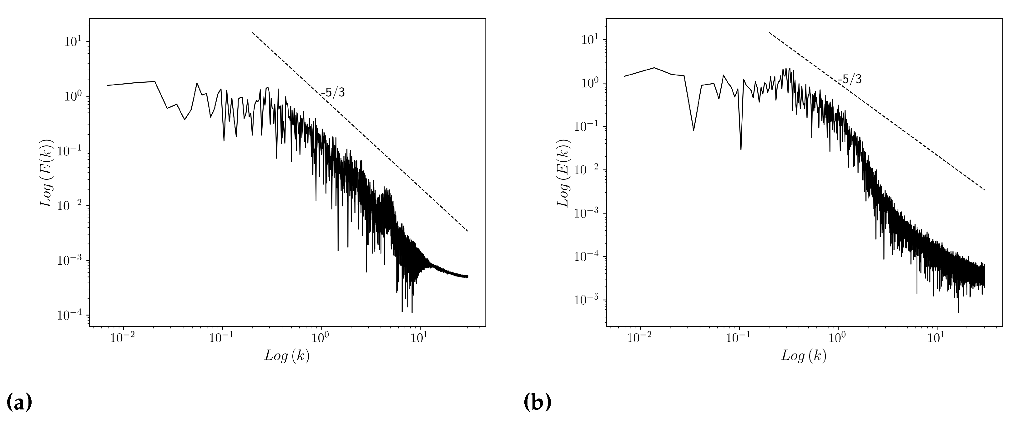By keeping that in mind, a validation process enabled the definition of the appropriate configuration of cells near the cylinder, able to reduce the discrepancy between the RMS lift coefficient and the Strouhal number predicted by the CFD simulation and the experimental values given by [15]. Likewise, the mesh capability to solve the turbulent kinetic energy is accounted from measuring the trend of the kinetic energy spectrum solved by the model on probe points at 1D and 1.5D downstream from the cylinder; these probes should describe a slope of -5/3 according to the Kolmogorov theory [24].

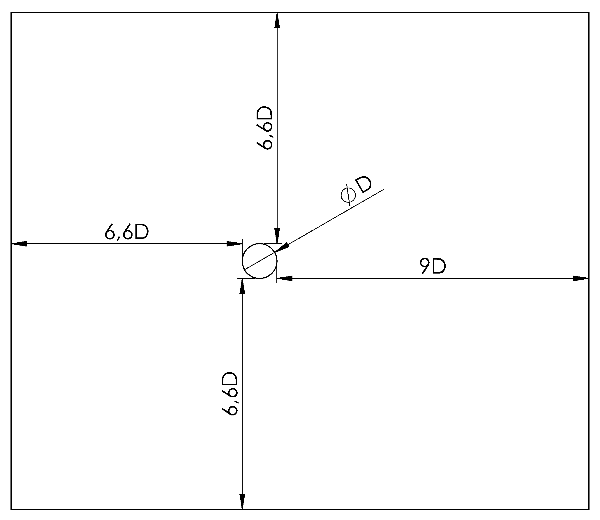
The validation considers a 3D simulation of an open flow crossing a cylinder of 0.3m in diameter with a Reynolds number equal to 72500 (see Section 1). Figure 8 represents the side view of the evaluated domain, whose dimensions depend on the cylinder diameter (D), including its depth, which is three times the cylinder diameter (3D), as recommended by [26].

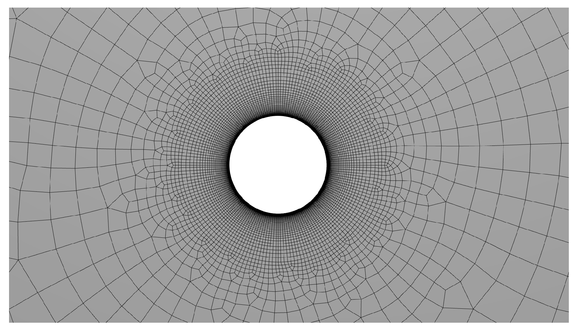
Figure 9 shows the discretisation of the domain in the vicinity of the cylinder. The implemented mesh has non-structural hexahedral elements and prismatic cells near the wall. Moreover, the discretisation assures a maximum aspect ratio of 100 near the cylinder and a growing factor of 1.2.

3.2.4. Latin Hypercube Sampling (Design of Experiment)

Engineers commonly use LES for the CFD evaluation of turbulent flow, thanks to the evolution of modern computers, which allow increasing the number of cells implemented during the domain discretisation while keeping a reasonable time on the running of studied cases. However, its individual implementation in optimisation, although possible [27], is still a challenge, as the processing time applies to a relevant number of configurations that trace the searching path toward the optimum condition. A common alternative to overcome this issue involves a design of experiments (DoE) with a limited number of simulations N, but adequate to construct a surrogate model to predict the studied variables’ response in places different from the samples evaluated using CFD [28].

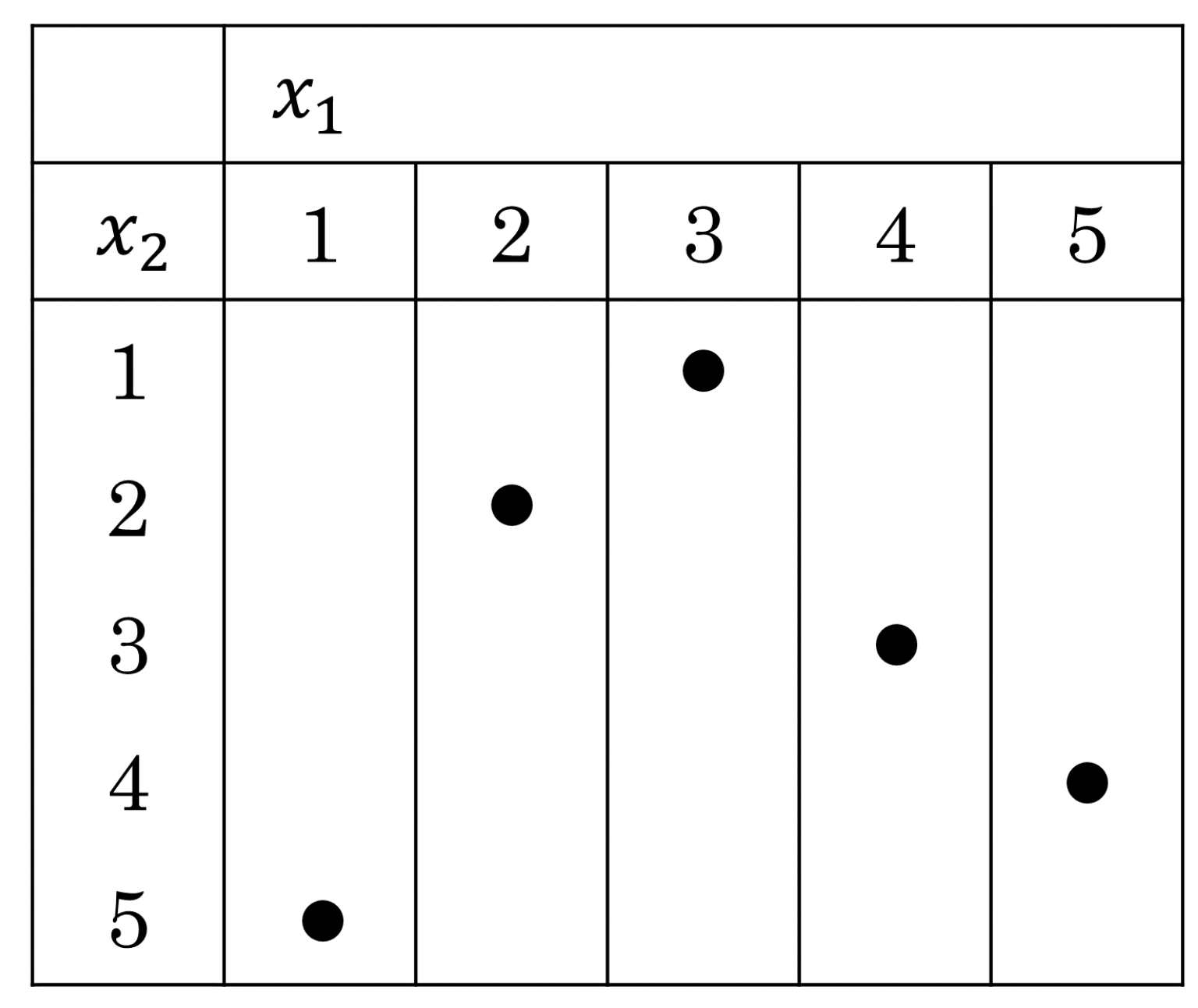
The dataset considered to build the surrogate model comes from a Latin Hypercube sampling (LHS) of two independent variables, L and S. In this sampling method, a square grid containing only a single sample by each row and column is constructed. The evaluation range of each variable is split into equal intervals to get the same number of sample points by variables (see Figure 10) [29].

In this study, S changes between

1 D \geq S \geq 7 D

and L between

0.5 D \geq L \geq 2 D

. The plate width is 0.2D, and the initial size of the sampling is 15 points per variable, a value above the minimum number recommended by [28].

3.2.5. CFD - cylinder plate evaluation

For the cylinder-plate cases, the domain suffers modifications because of the addition of the plate. However, the new mesh preserves the same characteristics defined in the vortex shedding validation process near the cylinder by keeping a growth ratio of 1.2 across the domain walls and a better aspect ratio. All of this assures a good prediction of the boundary layer.

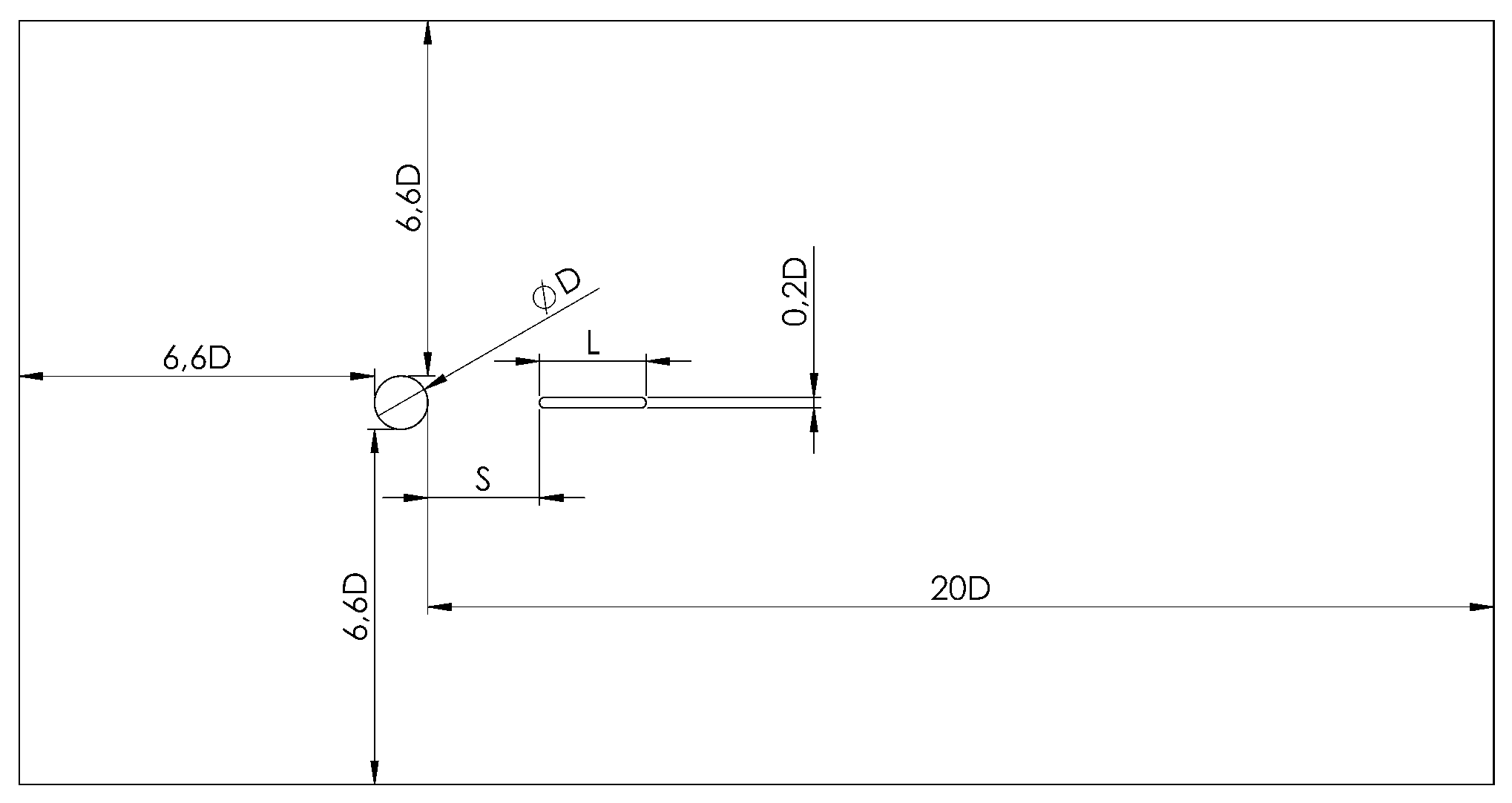
Figure 11 shows the parametric dimensioning of the CFD domain according to the diameter of the cylinder (D), where S is the distance between the plate and the cylinder, and L is the plate length. In addition, the width of the domain (direction normal to the section shown in Figure 11) is three times the diameter of the cylinder (3D), as recommended by [26].

3.2.6. Surrogate Model and Vortex Shedding Suppression

Among the mathematical functions available to build a surrogate model, radial basis functions have a track record in the field. Their general format contains a constant term

μ

and a localised deviation

M (x)

that considers the sampling data from the design of experiments [30] (see Eqn. 9).

y (x) = μ + M (x)

(9)

This work applies the Kriging interpolation function as a radial basis function to predict configurations that maximise the RMS lift coefficient of an aerodynamic plate whose position is downstream of a cylinder.

M (x)

in the Kriging Model tackles the covariance of the sampling

σ^{2}

and a correlation function derived from it. Different codes are available to construct the Kriging Model. But in this case, the outcomes come from a Python code developed by PyKrige, an in-deep description of the Kriging interpolation function is found in [28,30], while [31] offers a description of the Python library.

Equation 10, moreover, allows measuring the surrogate model accuracy, as it comes from the leave-one-out cross-validation (LOOCV) strategy. This equation employs a normalised root-mean-square error (

N R M S E

) of the model’s predictions, where

\hat{y}

represents the predicted response, y denotes the actual value, and i is a sample from the available universe of n samples. In addition,

y_{m a x}

and

y_{m i n}

are the maximum and minimum values of y, computed from the sampling points using CFD.

N R M S E = \frac{\sqrt{\frac{\sum_{i = 1}^{n} {({\hat{y}}_{i} - y_{i})}^{2}}{n}}}{(y_{m a x} - y_{m i n})}

(10)

The Kriging interpolation function is an appropriate tool for predicting variable response under different conditions. But this is only possible if objective functions behave as continuous functions through the design space. Unfortunately, the experiment results can describe some discontinuities because of an instantaneous zero-lift condition when the aerodynamic surface gets closer to the pole since it can break the vortex dynamics, a phenomenon known as vortex shedding suppression, reported by [32,33].

Based on the above, a decision tree classifier (DTC) algorithm allows filtering regions where the vortex shedding suppression occurs, across the design space, before building the Kriging interpolation function. The sampling reduction given by the filtering is handled by including a new set of samples able to tackle regions with a large discrepancy between the surrogate model and the CFD results when implementing the leave-one-out technique. The library PyKriging, available in Python, can perform this process [34].

3.3. Structural Dynamics Modelling

Newton’s Second Law dictates the dynamics of bladeless generators, as exemplified by Eqn. 11, which describes the dynamics of an aero generator from a rotational framework perspective. This equation involves several parameters, including

I_{0}

as the inertia,

C_{T}

as the damping coefficient,

K_{T}

as the restoration coefficient,

M_{(t)}

as the fluctuating external torque, and

θ

as the plate angular position. [3] studied the dynamic of Bladeless generators using an equivalent equation for translational systems.

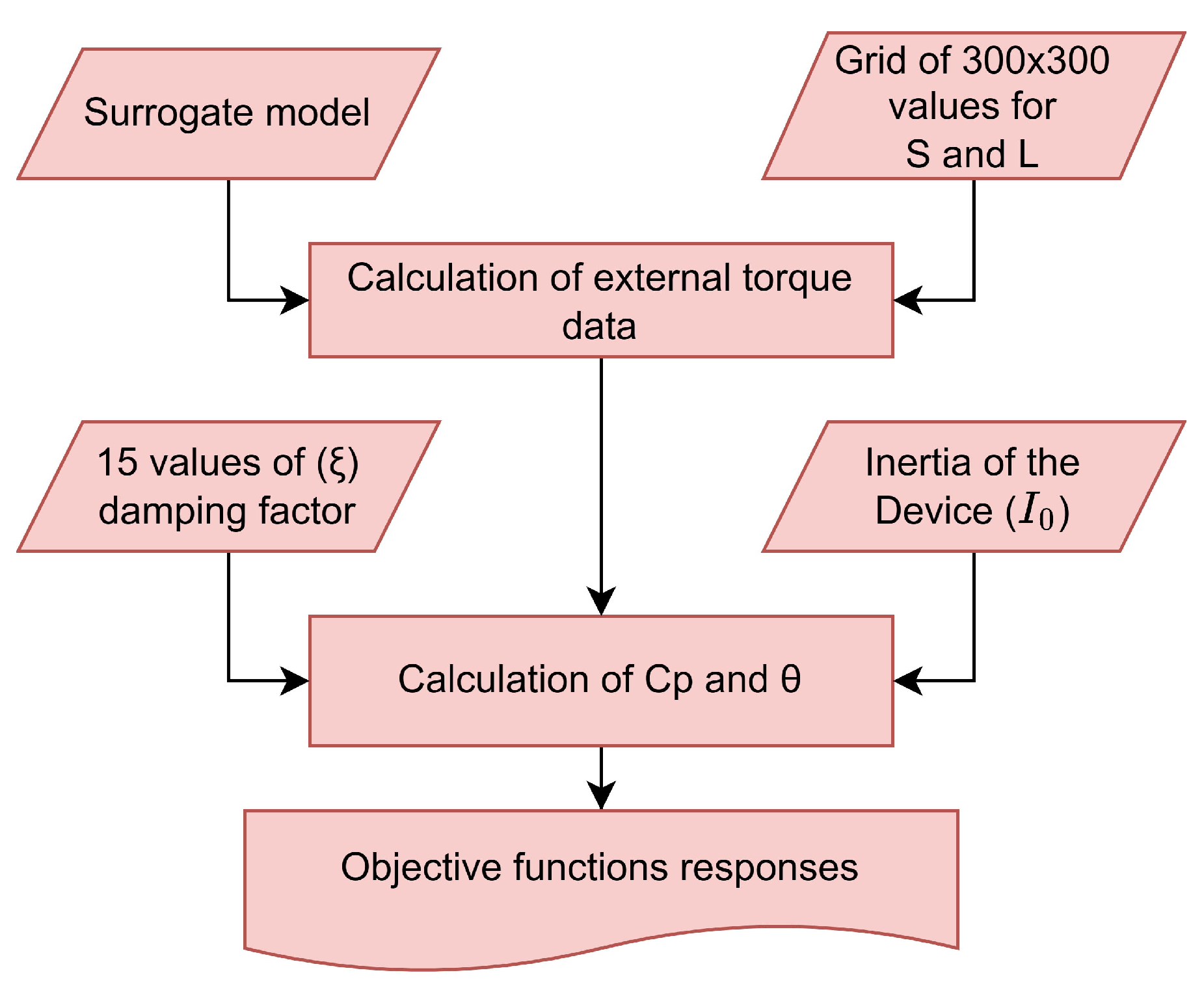
Figure 12, moreover, shows a schematic representation that helps understand the coupling of the surrogate model with the structural dynamics model to predict the values achieved by the studied objective function.

I_{0} \ddot{θ} + C_{T} \dot{θ} + K_{T} θ = M_{(t)}

(11)

The response of the vibrating system to external driving forces is mainly constrained by the magnitude of the damping and restoration forces, as well as by the characteristics of the driving force [16]. Bladeless generators, however, must operate in a narrow condition of resonance to achieve a maximum power conversion. Therefore, designers must fine-tune the vibratory system by selecting appropriate

C_{T}

and

K_{T}

values, according to the external force.

Based on the above, Eqn. 12 and Eqn. 13 provide an analytical solution to Eqn. 11 when the device operates at resonance. These two equations specify the device’s angular displacement and rotational velocity[35]. Their instantaneous values depend on several parameters of Eqn. 11, including

ω_{f}

, which relies on the vortex shedding frequency during resonance, as described in Eqn. 14, and the damping factor

ξ

θ_{(t)} = [\frac{M_{0}}{ω (2 ξ I_{0} ω_{f})}] s i n (ω_{f} t - \frac{π}{2})

(12)

{\dot{θ}}_{(t)} = [\frac{M_{0}}{2 ξ I_{0} ω_{f}}] c o s (ω_{f} t - \frac{π}{2})

(13)

ω_{f} = 2 π f_{f}

(14)

Meanwhile, Eqn. 15 and Eqn. 16 enable the calculation of the torque generated at the plate and the RMS power when a force applied at the centroid of the element replaces the load on it. The solution of these equations comes from integrating developed surrogate models (see Section 3.2.6), aimed to predict the values of

C l

and

f_{f}

based on different values of S and L.

\begin{matrix} M_{(t)} = [M_{0}] s i n (ω_{f} t) = \frac{[\sqrt{2} C l^{'} A ρ {V_{\infty}}^{2}]}{2} \\ (S + \frac{L}{2}) s i n (ω_{f} t) \end{matrix}

(15)

P o w_{m e c h R M S} = \frac{\int_{0}^{\infty} M_{(t)} {\dot{θ}}_{(t)} d t}{t}

(16)

Under a resonance condition, it is possible to show that the solution of Eqn. 16 depends on the plate inertia

I_{0}

, the damping factor

ξ

, the fluctuating external-torque amplitude

M_{0}

, and its frequency

ω_{f}

, as indicated in Eqn. 17.

P o w_{m e c h R M S} = \frac{{M_{0}}^{2}}{4 ξ I_{o} ω_{f}}

(17)

Equation 12 and Eqn. 17 involve only four variables to evaluate the dynamic responses of the device. These variables include the inertia

I_{0}

, which remains constant and equal to 10

k g m^{2}

, according to the implemented materials and plate sizes, the damping factor, the plate separation, and the plate length

(S + L)

; The damping factor changes within a feasible range of operation conformed by 15 different values, while the lift force and frequency comes from 300 configurations set with random values of S and L, uniformly distributed along the evaluation range.

3.4. Optimisation Process

The optimisation process is the final stage of the methodology. It requires constructing surrogate models to link S and L with

C l

and

f_{f}

and a code that solves Eqn. 5 and Eqn. 13 for different

ξ

, to describe the structural dynamics of the device. Figure 13 illustrates the methodology developed in this sub-stage, and the subsequent subsection describes the weighted global criterion method that allows for defining the Pareto frontier

3.4.1. The weighted global criterion method

The weighted global criterion method is a transformation option that combines multiple objective functions in a singular format for a general minimisation.

Eqn. 18 presents the most common weighted global criterion [36]. In this equation, U is the minimisation function,

f_{i} (x)

is an independent objective function evaluated on x,

f_{i}^{o}

is the utopic value of the objective function,

w_{i}

is a weight factor of an objective function, and p is a parameter of the model that measures the relevance of minimising the U function with the highest difference between

f_{i} (x)

and

f_{i}^{o}

. Therefore, large values of p (theoretically infinite) allow identifying points on the Pareto frontier for each combination of weights, whether this frontier presents a convex or non-convex curvature.

U = {\{\sum_{i = 1}^{k} {[w_{i} (f_{i} (x) - {f_{i}}^{o})]}^{p}\}}^{\frac{1}{p}}

(18)

Objective functions can display different orders of magnitude, which prompt the occurrence of numerical errors due to the nature of computers. Eqn. 19, however, allows for reducing this type of error by scaling the objective functions, as indicated by [36]. This equation includes the utopic value

(f_{i}^{o})

and the maximum value achieved by the studied objective function

(f_{i}^{m a x})

, both needed to have a scale of normalised values.

U = {\{\sum_{i = 1}^{k} {[w_{i} (\frac{f_{i} (x) - {f_{i}}^{o}}{{f_{i}}^{m a x} - {f_{i}}^{o}})]}^{p}\}}^{\frac{1}{p}}

(19)

Finally, Eqn. 20, allows computing the utopian values

f_{i}^{o}

, where

{(f_{i}^{o})}^{'}

represents a restrictive condition of the apparatus,

{(f_{i})}_{m i n}

the minimum value of the objective function in generated data, and

α

is a user-setting parameter that depends on the level of performance required in the design.

{f_{i}}^{o} = {({f_{i}}^{o})}^{'} + α [{(f_{i})}_{m i n} - {(f_{i}^{o})}^{'}]

(20)

4. Results Analysis

4.1. Mesh Sensitivity Analysis

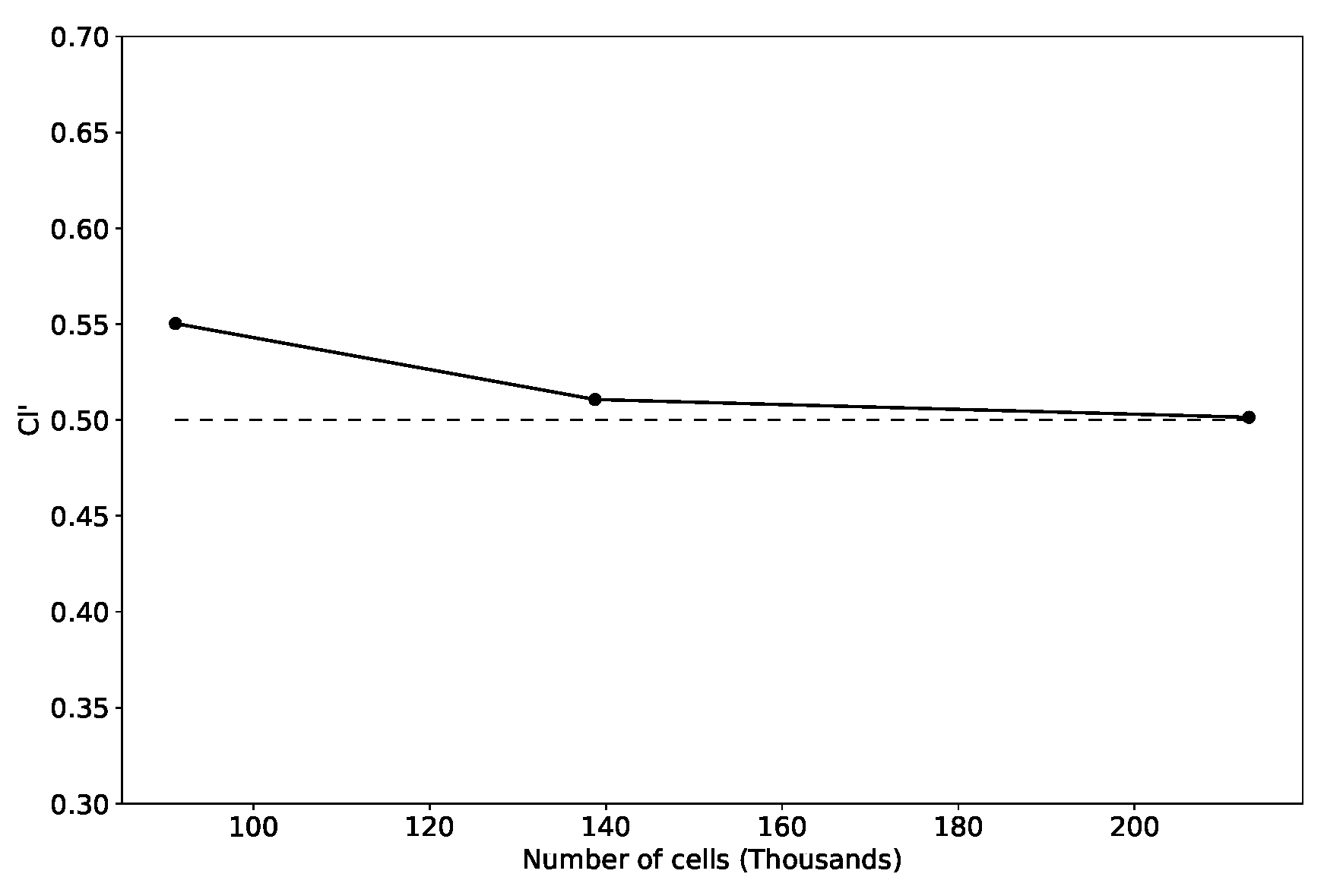
The domain discretisation started with 91155 cells, according to Section 3.2.3, and incremented its resolution with a factor of 1.5 on each test during the sensitivity analysis (see Table 4). Meanwhile, discrepancies between the Lift Coefficient and the Strouhal number computed by CFD and reported by [15] allowed for assessing their performance.

Figure 14 displays a graphical representation of the lift coefficient (

C l^{'}

) predicted from CFD using the discretisation detailed in Table 4 and Table 5, on the other hand, presents the CFD results for the lift coefficient, Strouhal number, and computed error between CFD and experimental data [15]. The CFD simulations always overestimate the RMS lift coefficient, while the Strouhal number exhibits oscillatory behaviour. Out of all the cases, Case 3 produces the most accurate results with a percentage error of less than 1% for both the lift coefficient and the Strouhal number. Based on these results, Case 3 works as the baseline discretisation during the optimisation.

Figure 15 illustrates the Kolmogorov energy spectrum computed from the instantaneous velocity field measured by two probes located downstream from the cylinder at distances of

1 D

and

1.5 D

, using the mesh resolution from case 3. The graph also shows a dashed line with a slope of

\frac{- 5}{3}

to represent the typical energy spectrum trend at the inertial scale. A simple comparison of trends confirms that the LES filter is small enough within the studied region.

4.2. Aerodynamic behaviour of the cylinder-plate configuration

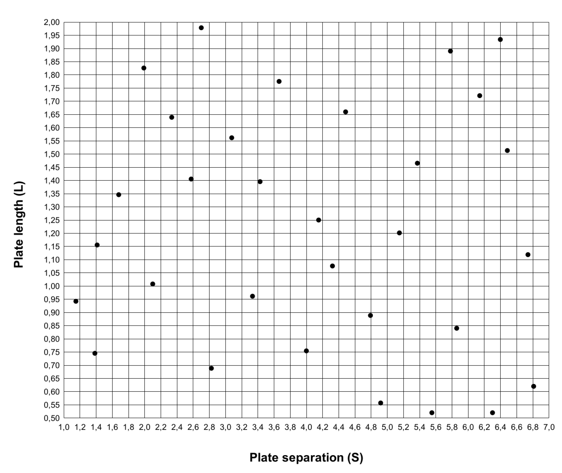
The aerodynamic study of the cylinder-plate configuration implemented a DOE according to Section 3.2.4. Figure 16 shows the sampling location, where S and L represent the cylinder-plate separation and plate length (see Figure 11).

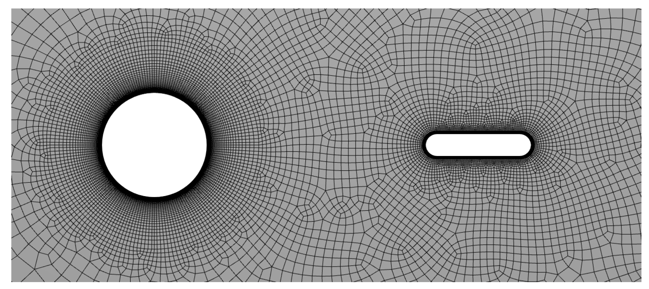
Figure 17 shows an example of the mesh used in the CFD evaluation. The number of inflation layers near the plate is 22, with 1.15 as the growth rate. The cases studied maintain a mesh resolution equal to Case 3 in the neighbourhood of the cylinder to provide a good prediction of vortex-shedding.

Figure 18 shows an instantaneous value of the fluid vorticity. Case (a) represents a scenario where vortex shedding occurs. Case (b), moreover, represents a scenario where vortex suppression appears due to the plate’s proximity to the cylinder. The classification method described in the Section 3.2.6, with a decision boundary of

C l^{'} \geq 0.45

, allows for discarding the suppression condition.

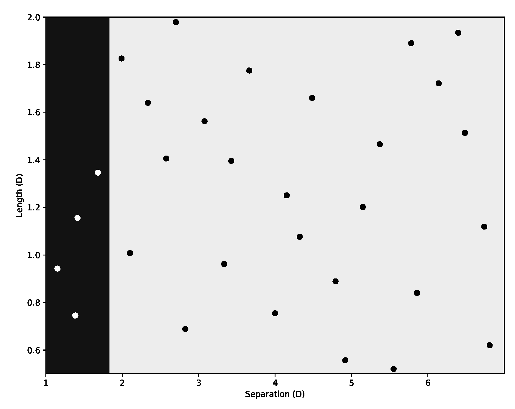
Figure 19 presents the outcomes from the classification method. The black region represents the design space where the vortex shedding suppression occurs (

S / D \leq 1.83

). Eliminating the vortex shedding suppression region modifies the evaluation range of cylinder-plate separation to

1.83 \geq S / D \geq 7

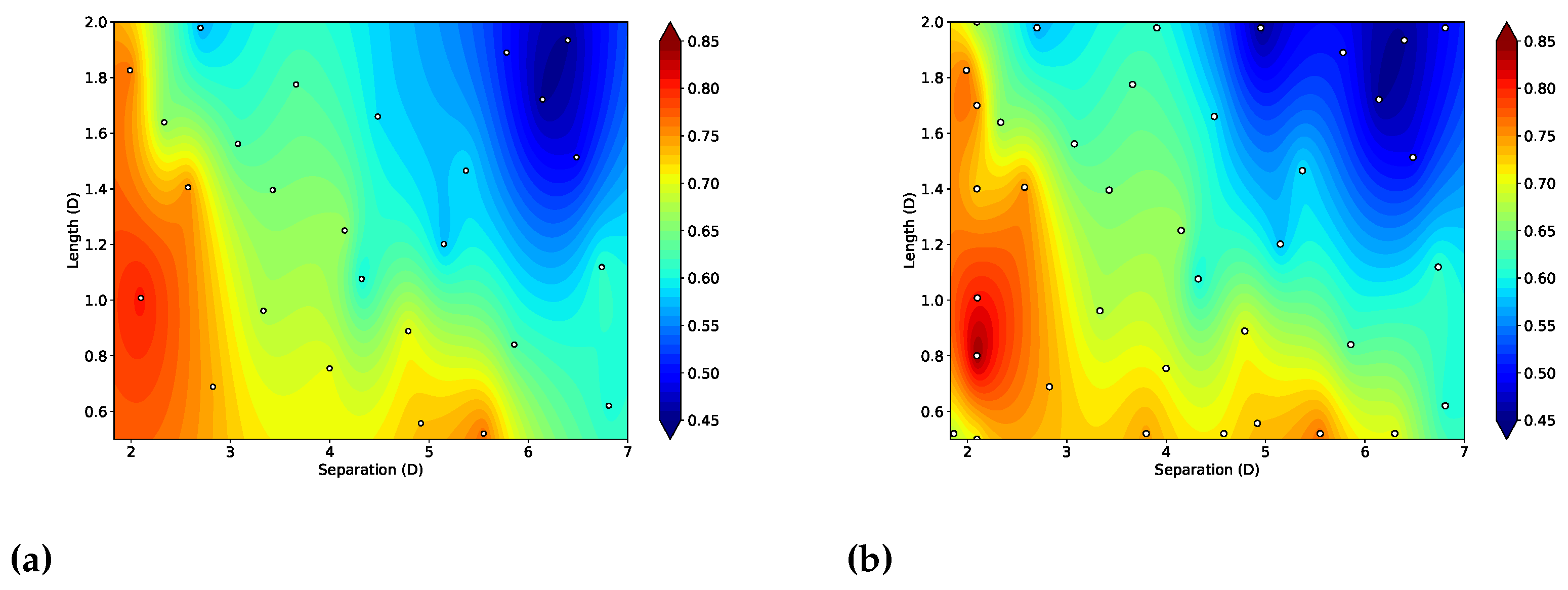
and reduces the number of samples to 26 (13 per variable). With this smaller dataset, a Kriging model to predict

C l^{'}

allowed an NRMSE of

15.5 %

during the implementation of the lift-one-out technique. However, the addition of 12 new samples, located in regions that had high errors during the surrogate model validation process, allowed for maintaining the original sample size and a final reduction of the NRMSE to

12.42 %

Figure 20 displays the contour plots of

C l^{'}

before and after the implementation of the sampling enhancement. The new samples do not significantly alter the overall patterns within the design space. However, they improve the localised resolution of specific areas, resulting in a more accurate estimation of the maximum and minimum values of

C l^{'}

, which allows a better prediction of the optimal Power Coefficient.

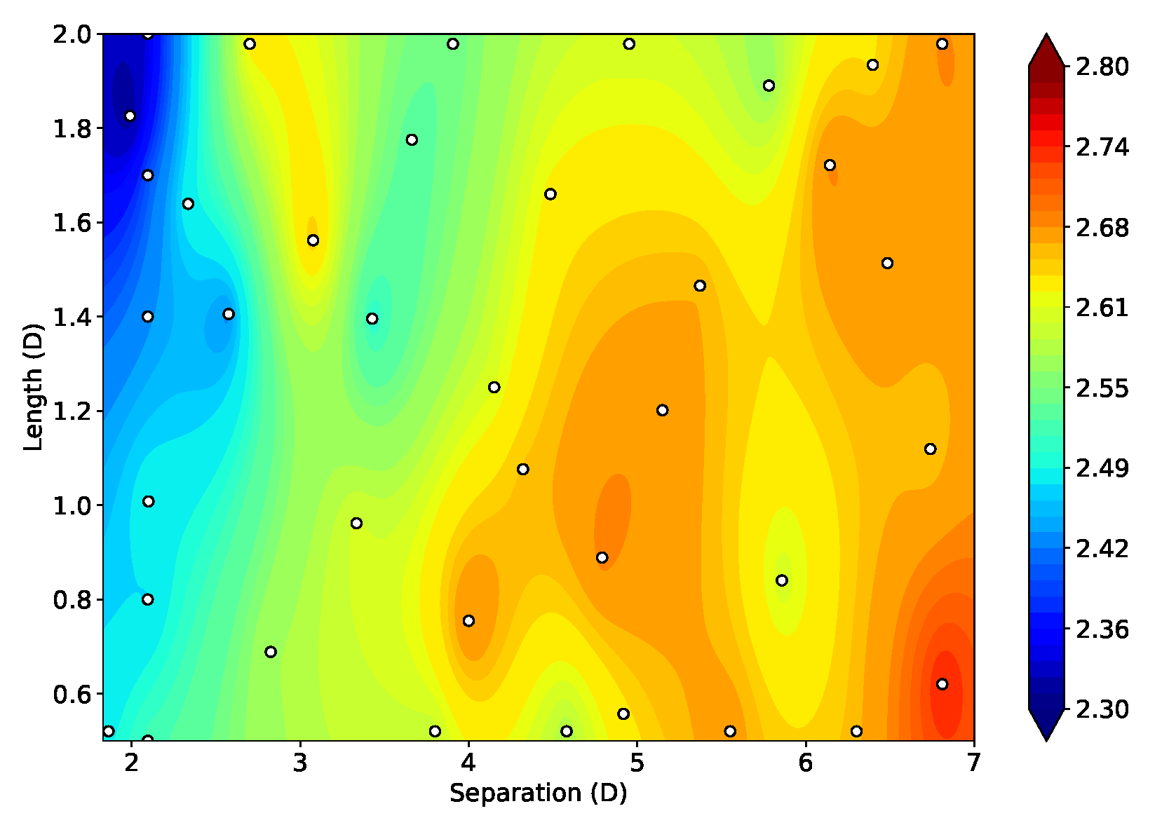
Concerning the vortex shedding frequency, Figure 21 displays its contour plot using the resulting 38 samples from the validation process mentioned above. For this variable, the Kriging model is capable of predicting values with an NRMSE of

13.08 %

4.3. Structural behaviour of the cylinder-plate configuration

The following results come from executing the procedures outlined in Section 3.3. The aim is to determine a potential increment in the device’s power coefficient

(F_{1})

and a decrement in its displacement

(F_{2})

while changing the damping factor value between 0.01 and 0.05. Furthermore, good optimisation practices seek to define objective functions that require minimisation. In this study, therefore, the reduction in the ratio of unused energy

(1 - C_{p})

replaces the device power coefficient

(C_{p}

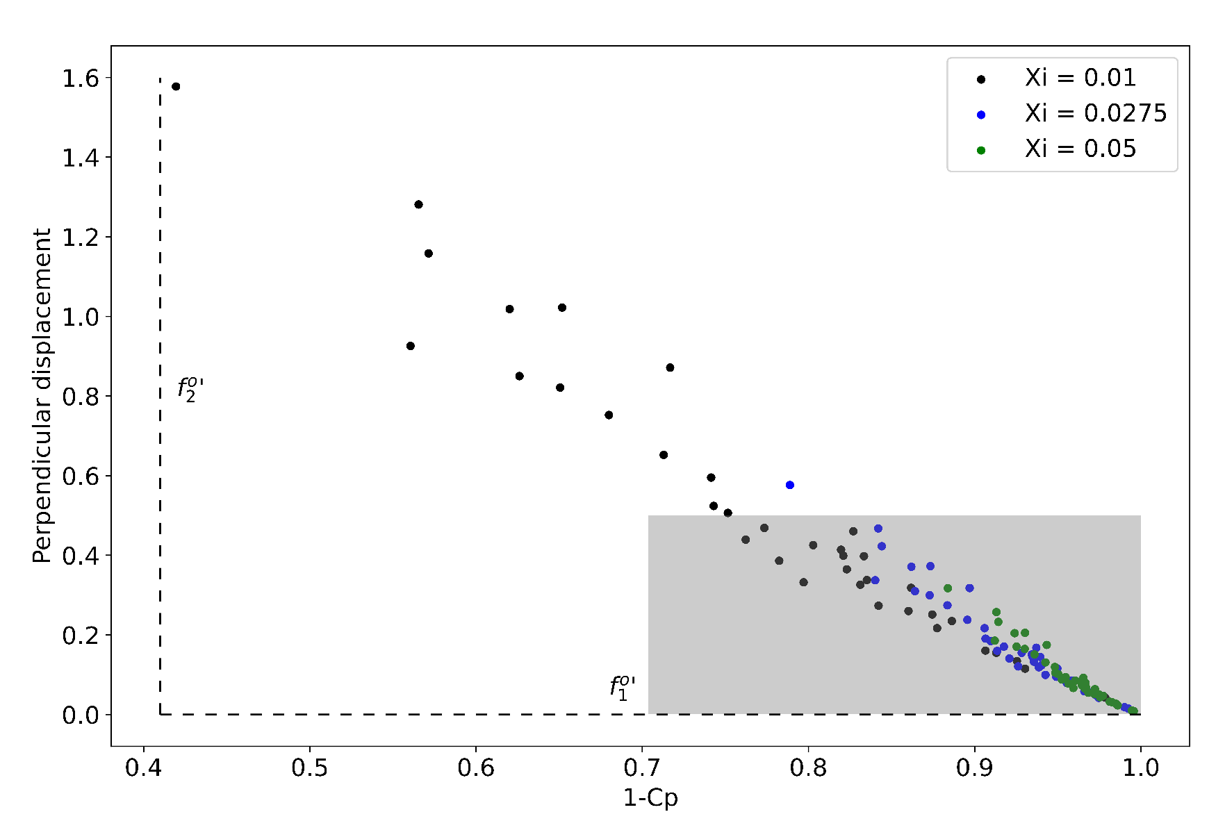
Figure 22 shows the response of the oscillating system according to Newton’s Second Law of Motion for the different values of the damping factor, plate length, and cylinder separation. The dashed lines in the figure indicate the machine’s restrictive conditions;

{F_{1}^{0}}^{'}

0.41

, and corresponds to the minimum ratio of unused energy, according to the momentum theory - Benz law [37], while

{F_{2}^{0}}^{'}

is zero and corresponds to the minimum displacement condition of the system, achieved at elevated damping coefficient. The grey frame, meanwhile, defines the criterion space according to the utopian

({F_{i}}^{0})

and critical

(F_{i}^{C})

values of objective functions; the utopian values come from Eqn. 20 when

α

is equal to

0.9

, while critical values are

0.5 D

for the lateral displacement and 1 for the ratio of unused energy, indicating the not production of Power.

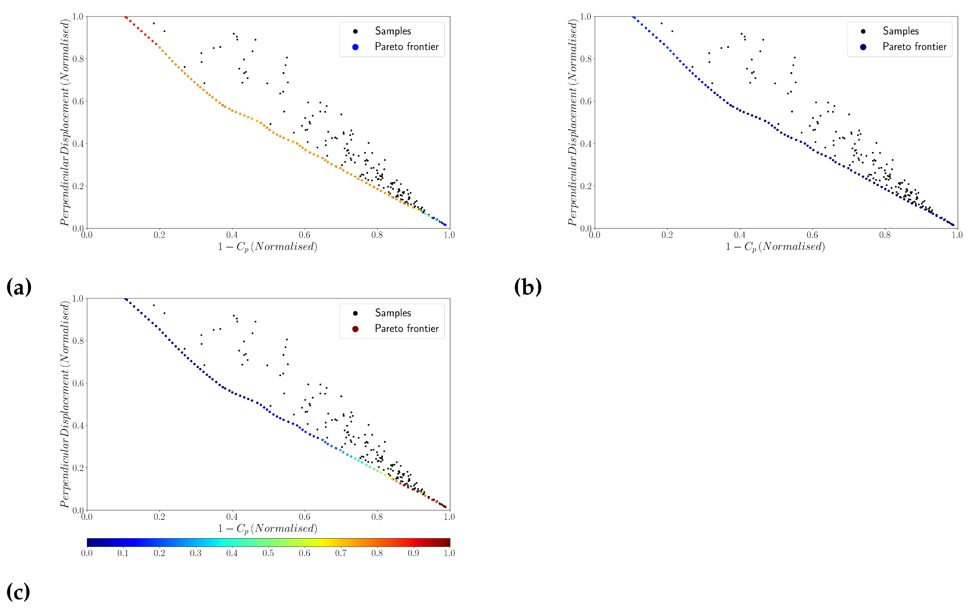
Figure 23 displays the normalised values of the perpendicular displacement and the ratio of unused energy obtained from the data within the grey box of Figure 22; the normalisation considers the machine’s restrictive conditions (

{F_{i}^{0}}^{'}

) and critical values (

F_{i}^{C}

). Equ.19 allows computing the Pareto frontier of this figure using a p equal to 145, a value high enough to perform the optimisation while avoiding any relevant computer round-off errors. The weighting factor changes from 0 to 1 with a step size of 0.1, while colours in the Pareto frontier represent the variables S, L, and

ξ

, respectively.

Figure 23 indicates that a cylinder plate separation between

0.7

and

0.8

represents an extensive part of the Pareto frontier. However, large values of this variable give a high-power coefficient and a high perpendicular displacement of the device. Conversely, a lower value for this variable leads to the opposite effect. Furthermore, the plate length shows consistent variations throughout the Pareto frontier, with values mainly ranging between

0.45

and 0. Finally, most points on the Pareto frontier report low values of

ξ

. However, high values of this variable significantly reduce the perpendicular displacement of the device.

The Euclidean distance calculation between the computed and the utopian condition allows for determining the scenario that provides the ideal outcome based on the weighting factors. Table 6 shows six optimum configurations as follows. The first and the last row presents the optimum condition after considering the perpendicular displacement or the ratio of unused energy alone. The other rows represent the multi-objective optimal scenarios, where the third row exhibits the minimum Euclidean distance calculated from all of the evaluated conditions.

In Cases 2, 3, and 4, the distance between the pole and the plate remains almost constant. However, as the length increases,

F_{1}

decreases while

F_{2}

increases. On the other hand, the damping coefficient produces the opposite effect. Case 5 gives the maximum power coefficient, with a value of

0.267 (1 - F_{1})

, but it also produces the maximum displacement. By selecting Case 3 as the optimal choice, the desired configuration requires a plate with a length of

0.52 D

, a separation of

5.548 D

from the cylinder, and a damping factor of

0.013

. This design results in a perpendicular displacement of

0.226 D

(normalised:

0.451 D

) and a ratio of unused energy of

0.853

(normalised:

0.513

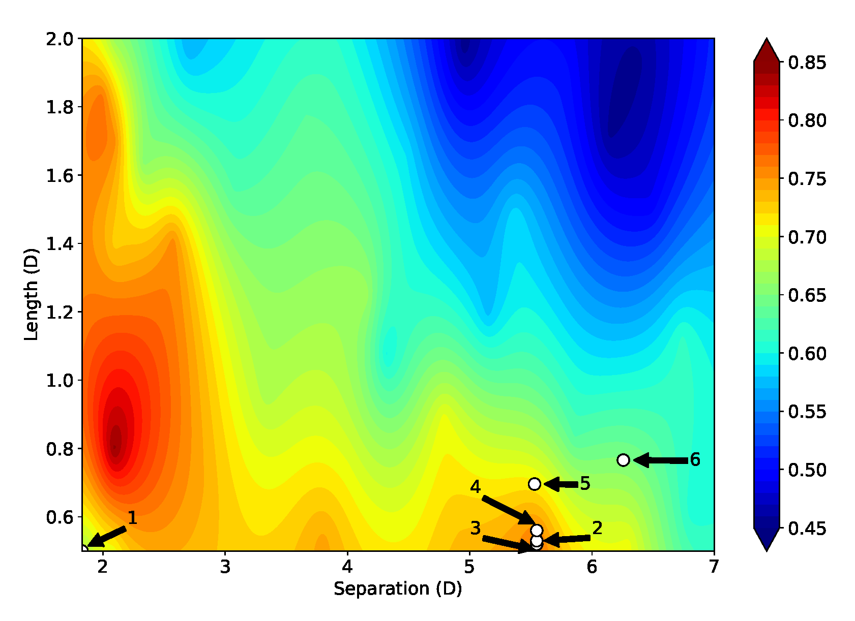
Figure 24 illustrates the configurations presented in Tab. Table 6 and the

C l^{'}

contour. It is worth noting that there is a significant disparity between condition one and the others; this may be due to the prioritisation of displacement reduction in condition one without considering the energy generated. In contrast, the remaining cases are in a region where the lift coefficient varies from moderate to high, particularly in cases 2, 3 and 4. These findings indicate that the lift coefficient plays a critical role in the optimisation process of these generators, especially when the design aims to achieve compactness and high power coefficients.

5. Conclusions

After reviewing the results of this study, it can be concluded that:

The Kriging surrogate model and a classification method allowed identifying a zone within the sampling space where vortex suppression occurs. To prevent this effect, a gap between the plate and the cylinder must be higher than $1.83 (\frac{S}{D})$ .
Results from the multi-objective optimisation showed that, under the given constraints, this type of wind generator produces a power coefficient of up to $0.269$ when its oscillation amplitude is at its maximum $(0.5 D)$ . Moreover, from all the evaluated configurations, a design with $ξ = 0.013$ , $\frac{S}{D} = 5.548$ and $\frac{L}{D} = 0.520$ provide the closest match to the utopian condition.
Finally, the results obtained in this study suggest that the configuration with the minimum Euclidean distance to the Pareto frontier offers an increase of $15.38 %$ in the value of the power coefficient concerning the Vortex Nano bladeless generator in similarly windy conditions.

Author Contributions

The work was conceptualised by G.M. and A.S., who provided guidance to the group throughout the process. A.O., S.R., and J.Z. constructed the CFD model, designed the experiments, and post-processed the computational results. The original draft was written by G.M. and subsequently edited by all authors. All authors have read and agreed to the published version of the manuscript.

Funding

This research received no external funding.

Institutional Review Board Statement

“Not applicable” for studies not involving humans or animals.

Informed Consent Statement

“Not applicable”

Acknowledgments

The authors desire to express their sincere gratitude to SimScale for providing access to their HPC system, which was essential in carrying out the simulations presented in this paper. The invaluable support and assistance of the SimScale team have been instrumental in achieving the research goals of this study. This generous contribution is a testament to the exceptional quality of the organisation. The authors extend their heartfelt thanks to SimScale for their invaluable assistance and support.

Conflicts of Interest

Declare conflicts of interest or state “The authors declare no conflict of interest. “The funders had no role in the design of the study; in the collection, analysis or interpretation of data; in writing the manuscript; or in the decision to publish the results”.

Abbreviations

$F_{L}$	Lift force
$ρ$	Density
$V_{\infty}$	Free stream velocity
s	Surface area
S	Separation distance
L	Plate length
$C l^{'}$	RMS lift coefficient
f	Vortex shedding frequency
l	Characteristic length
$I_{0}$	Inertia
$C_{T}$	Damping coefficient
$K_{T}$	Restoration coefficient
$θ$	Position
$M_{0}$	External torque
$ω_{F}$	External torque frequency
$ξ$	Damping factor
U	Minimisation function
$f_{i}^{0}$	Utopic value
$f_{c}^{0}$	Critical value
$w_{i}$	Weight factor of objective function
p	Minimisation function parameter
$f_{i}^{m a x}$	Maximum value of objective function
$f_{i}^{m i n}$	Minimum value of objective function
$α$	User setting for level of performance required

References

Sumathi, S.; Kumar, L.; Surekha, P. Solar PV and Wind Energy Conversion Systems: An Introduction to Theory, Modeling with MATLAB/SIMULINK, and the Role of Soft Computing Techniques; Green Energy and Technology, Springer International Publishing:, 2015. [Google Scholar]
Hau, E.; Renouard, H. Wind Turbines: Fundamentals, Technologies, Application, Economics; SpringerLink: Bücher, Springer: Berlin/Heidelberg, 2013. [Google Scholar]
Yáñez Villarreal, D.J. Viv resonant wind generators - vortex bladeless wind power, 2018.
Cajas García, J.C.; Houzeaux, G.; Yáñez, D.J.; Mier-Torrecilla, M. SHAPE Project Vortex Bladeless: Parallel multi-code coupling for Fluid-Structure Interaction in Wind Energy Generation, 2016.
Francis, S.; Umesh, V.; Shivakumar, S. Design and Analysis of Vortex Bladeless Wind Turbine. Materials Today: Proceedings 2021, 47, 5584–5588. [Google Scholar] [CrossRef]
Mane, A.; Kharade, M.; Sonkambale, P.; Tapase, S.; Kudte, S.S. Design & analysis of vortex bladeless turbine with gyro e-generator. International Journal of Innovative Research in Science and Engineering 2017, 3, 445–452. [Google Scholar]
Chizfahm, A.; Yazdi, E.A.; Eghtesad, M. Dynamic modeling of vortex induced vibration wind turbines. Renewable Energy 2018, 121, 632–643. [Google Scholar] [CrossRef]
Shahat, A.E.; Hasan, M.; Wu, Y. Vortex Bladeless Wind Generator for Nano-Grids. 2018 IEEE Global Humanitarian Technology Conference (GHTC), 2018; 1–2. [Google Scholar]
Tandel, R.; Shah, S.; Tripathi, S. A state-of-art review on Bladeless Wind Turbine. Journal of Physics: Conference Series 2021, 1950, 012058. [Google Scholar] [CrossRef]
Aballe, A.B.D.; Cruz, K.Y.C.; Rosa, V.J.H.D.; Magwili, G.V.; Ostia, C.F. Development of a Linear Generator With Spring Mechanism for Vortex Bladeless Wind Turbine. 2020 IEEE 12th International Conference on Humanoid, Nanotechnology, Information Technology, Communication and Control, Environment, and Management (HNICEM), 2020, pp. 1–6. [CrossRef]
Ordoñez, O.; Duke, A.R. Wind Resource Assessment: Analysis of the Vortex Bladeless Characteristics in Puerto Cortés, Honduras. IOP Conference Series: Earth and Environmental Science 2021, 801, 012019. [Google Scholar] [CrossRef]
ELDREDGE, J.D.; PISANI, D. Passive locomotion of a simple articulated fish-like system in the wake of an obstacle. Journal of Fluid Mechanics 2008, 607, 279–288. [Google Scholar] [CrossRef]
Wu, J.; Shu, C. Numerical study of flow characteristics behind a stationary circular cylinder with a flapping plate. Physics of Fluids 2011, 23, 073601. [Google Scholar] [CrossRef]
Wang, H.; Zhai, Q.; Zhang, J. Numerical study of flow-induced vibration of a flexible plate behind a circular cylinder. Ocean Engineering 2018, 163, 419–430. [Google Scholar] [CrossRef]
Norberg, C. Fluctuating lift on a circular cylinder: review and new measurements. Journal of Fluids and Structures 2003, 17, 57–96. [Google Scholar] [CrossRef]
White, G. Introduction to Machine Vibration; Reliabilityweb.com, 2008.
The-SciPy-community. Fourier Transforms (scipy.fft), 2023.
Rao, K.R.; Yip, P. The Transform and Data Compression Handbook; CRC Press, Inc.: USA, 2000. [Google Scholar]
Cengel, Y.A.; Cimbala, J.M. Mecánica De Fluidos 4a Edición; Mcgraw Hill: 2018.
Damiána, S.M.; Nigro, N.M. COMPARISON OF SINGLE PHASE LAMINAR AND LARGE EDDY SIMULATION (LES) SOLVERS USING THE OPENFOAM R SUITE. Mecánica Computacional 2010, 29, 3721–3740. [Google Scholar]
Blazek, J. Computational Fluid Dynamics: Principles and Applications; Elsevier Science: 2015.
OpenCFD-Ltd. OpenFOAM User Guide: Smagorinsky, 2017.
Berselli, L.; Iliescu, T.; Layton, W. Mathematics of Large Eddy Simulation of Turbulent Flows; Scientific Computation, Springer, 2006. [Google Scholar]
Sagaut, P.; Meneveau, C. Large Eddy Simulation for Incompressible Flows: An Introduction; Scientific Computation, Springer, 2006. [Google Scholar]
GmbH, S. Large Eddy Simulation - Flow Over a Cylinder, accessed on 2023-03-08.
Cao, Y.; Tamura, T. Numerical investigations into effects of three-dimensional wake patterns on unsteady aerodynamic characteristics of a circular cylinder at Re=1.3×105. Journal of Fluids and Structures 2015, 59, 351–369. [Google Scholar] [CrossRef]
Spanelis, A.; Walker, A.D. A Multi-Objective Factorial Design Methodology for Aerodynamic Off-Takes and Ducts. Aerospace 2022, 9. [Google Scholar] [CrossRef]
Kleijnen, J.P. Design and Analysis of Simulation Experiments; International Series in Operations Research & Management Science; Springer, 2015. [Google Scholar]
Chen, V.C.; Tsui, K.L.; Barton, R.R.; Meckesheimer, M. A review on design, modeling and applications of computer experiments. IIE Transactions 2006, 38, 273–291. [Google Scholar] [CrossRef]
Simpson, T.W.; Poplinski, J.D.; Koch, P.N.; Allen, J.K. Metamodels for Computer-based Engineering Design: Survey and recommendations. Engineering with Computers 2001, 17, 129–150. [Google Scholar] [CrossRef]
Murphy, B.; Yurchak, R.; Müller, S. GeoStat-Framework/PyKrige: v1.7.0, 2022.
Akilli, H.; Sahin, B.; Filiz Tumen, N. Suppression of vortex shedding of circular cylinder in shallow water by a splitter plate. Flow Measurement and Instrumentation 2005, 16, 211–219. [Google Scholar] [CrossRef]
Dai, S.; Younis, B.A.; Zhang, H.; Guo, C. Prediction of vortex shedding suppression from circular cylinders at high Reynolds number using base splitter plates. Journal of Wind Engineering and Industrial Aerodynamics 2018, 182, 115–127. [Google Scholar] [CrossRef]
Chris, P.; Giorgos, R. pyKriging: A Python Kriging Toolkit, 2015.
Shabana, A. Theory of Vibration: An Introduction; Mechanical Engineering Series, Springer International Publishing: 2019.
Arora, J.S. (Ed.) Introduction to Optimum Design (Fourth Edition), 3rd ed.; Academic Press: Boston, 2011. [Google Scholar]
Sons, J.W.., Ed., The Wind Resource. In Wind Energy Handbook; Sons, J.W.., Ed.; John Wiley & Sons, Ltd: 2011; chapter 2, pp. 9–38. [CrossRef]

Figure 1. Power coefficients of different wind turbines [2].

Figure 2. Scheme of bladeless generators.

Figure 3. CAD model of the proposed concept of wind generator.

Figure 4. Domain configuration to assess the optimisation process.

Figure 5. methodological plan.

Figure 6. Graphic representation of perpendicular displacement.

Figure 7. Diagram of Surrogate Model Stage.

Figure 8. Domain configuration for the validation of the CFD model (free stream that crosses a cylinder).

Figure 9. Mesh with 181 divisions along the cylinder circumference.

Figure 10. LHS of two variables with 5 intervals [29].

Figure 11. Domain configuration to assess the effect of the Von Kármán Vortex Street on aerodynamic shapes.

Figure 12. Diagram of Structural Dynamics Modelling Stage.

Figure 13. Diagram of optimisation process methodology.

Figure 14. CFD trend on the

C l^{'}

prediction during the mesh refinement.

Figure 14. CFD trend on the

C l^{'}

prediction during the mesh refinement.

Figure 15. Kolmogorov energy spectrum post-processed from the instantaneous velocity field of Case 3 at a) 1D and b)1.5D downstream from the cylinder (wake zone).

Figure 16. Latin hypercube sampling.

Figure 17. Domain discretisation of a sample from the studied sampling.

Figure 18. Vorticity contour for samples a) without and b) with vortex suppression.

Figure 19. Decision tree classification of the sampling - decision boundary at 0.45 for the Cl’(black region reports the vortex shedding suppression).

Figure 20. Contour of Lift Coefficient

C l

- (a) Kriging function built from 26 samples and b) Kriging function built from 38 samples.

Figure 20. Contour of Lift Coefficient

C l

- (a) Kriging function built from 26 samples and b) Kriging function built from 38 samples.

Figure 21. Contour of

f_{f}

- Kriging function built from 38 samples.

Figure 21. Contour of

f_{f}

- Kriging function built from 38 samples.

Figure 22. Response of the Oscillatory System to Sampling: Analysis of Damping Factors (0.01, 0.0275 and 0.05) and Spatial Criteria.

Figure 23. Pareto frontier - the colour map indicates values of a) S, b) L, c)

ξ

along the frontier.

Figure 23. Pareto frontier - the colour map indicates values of a) S, b) L, c)

ξ

along the frontier.

Figure 24. Optimum conditions of Tab. Table 6 and the contour of lift coefficient

(C l)

built from 38 samples.

Figure 24. Optimum conditions of Tab. Table 6 and the contour of lift coefficient

(C l)

built from 38 samples.

Table 1. Fluid Properties.

Fluid	Air
$ρ (\frac{k g}{m^{3}})$	1.145
Dynamic Viscosity $(\frac{k g}{m s})$	$1.1895 E - 5$

Table 2. Boundary conditions.

Name	Type
Inlet	$4 \frac{m}{s}$ normal direction (free stream)
Outlet	Gauge pressure 0 Pa
Cylinder	Wall
Others	Symmetry

Table 3. Numerical settings.

Name	Type
CFD Model	LES 3D
Algorithm	PISO
Numerical Scheme	2nd Order Upwind
Sub-Grid Scale Model	Smagorinsky-Lilly
Time step	$2.5 E - 4 s$
Flow time	$12 s$

Table 4. Mesh configuration during the validation.

Case	Divisions	# Cells
1	74	91155
2	116	138765
3	181	212985

Table 5. CFD results comparison using [15] as the benchmark.

Case	Cl	St	Error Cl (%)	Error St (%)
Experimental	0.500	0.198	-	-
1	0.550	0.208	10.067	5.422
2	0.511	0.192	2.142	2.816
3	0.501	0.197	0.285	0.238

Table 6. Single and multi-objective optimum points.

Case	Weight	Euclidian	F1 value	F2 value	$ξ$	S/D	L/D
	$(F 1 - F 2)$	Distance	(normalised)	(normalised)		value	value
1	0.00 - 1.00	0.987	0.996 (0.987)	0.008D (0.016)	0.050	1.830	0.500
2	0.25 - 0.75	0.778	0.921 (0.739)	0.122D (0.244)	0.024	5.548	0.530
3	0.47 - 0.53	0.683	0.853 (0.513)	0.226D (0.451)	0.013	5.548	0.520
4	0.50 - 0.50	0.688	0.845 (0.488)	0.242D (0.485)	0.013	5.548	0.560
5	0.75 - 0.25	0.800	0.774 (0.252)	0.380D (0.759)	0.010	5.530	0.696
6	0.90 - 0.10	0.998	0.731 (0.109)	0.496D (0.992)	0.010	6.343	0.766

Disclaimer/Publisher’s Note: The statements, opinions and data contained in all publications are solely those of the individual author(s) and contributor(s) and not of MDPI and/or the editor(s). MDPI and/or the editor(s) disclaim responsibility for any injury to people or property resulting from any ideas, methods, instructions or products referred to in the content.

© 2023 by the authors. Licensee MDPI, Basel, Switzerland. This article is an open access article distributed under the terms and conditions of the Creative Commons Attribution (CC BY) license (http://creativecommons.org/licenses/by/4.0/).

Copyright: This open access article is published under a Creative Commons CC BY 4.0 license, which permit the free download, distribution, and reuse, provided that the author and preprint are cited in any reuse.

MDPI Initiatives

Important Links

Choose an area of interest and we will send you notifications of new preprints at your preferred frequency.

Disclaimer

Assessment of Aerodynamic Plates Subjected to Von Kármán Vortex Street for Enhancing the Wind Energy Generation in Blade-less Devices

Abstract

1. Introduction

2. The Studied Problem: Device’s Structural Dynamics Responses

3. Methodology

3.1. Studied variables

3.1.1. The Lift-Coefficient

3.1.2. The Strouhal number

3.1.3. The perpendicular displacement

3.1.4. The Power Coefficient

3.2. The Surrogate Model

3.2.1. CFD model

3.2.2. Model setup

3.2.3. CFD Vortex Shedding Validation

3.2.4. Latin Hypercube Sampling (Design of Experiment)

3.2.5. CFD - cylinder plate evaluation

3.2.6. Surrogate Model and Vortex Shedding Suppression

3.3. Structural Dynamics Modelling

3.4. Optimisation Process

3.4.1. The weighted global criterion method

4. Results Analysis

4.1. Mesh Sensitivity Analysis

4.2. Aerodynamic behaviour of the cylinder-plate configuration

4.3. Structural behaviour of the cylinder-plate configuration

5. Conclusions

Author Contributions

Funding

Institutional Review Board Statement

Informed Consent Statement

Acknowledgments

Conflicts of Interest

Abbreviations

References

MDPI Initiatives

Important Links

Subscribe