Preprint

Article

Investigating the Effects of Parameter Tuning on Machine Learning for Occupant Behavior Analysis in Japanese Residen-tial Buildings

Altmetrics

Downloads

Views

Comments

A peer-reviewed article of this preprint also exists.

This version is not peer-reviewed

Submitted:

17 May 2023

Posted:

18 May 2023

You are already at the latest version

Alerts

Abstract

In this study, machine learning was used to predict and analyze the behavior of occupants in Gifu City residences during winter. Global warming is currently progressing worldwide, and it is important to control greenhouse gas emissions from the perspective of adaptation and mitigation. Occupant behavior is highly individualized and must be analyzed to accurately determine a building's energy consumption. The accuracy of heating behavior prediction has been studied using three different methods: logistic regression, support vector machine (SVM), and deep neural network (DNN). The generalization ability of the support vector machine and the deep neural network was improved by parameter tuning. Parameter tuning of the SVM showed that the values of C and gamma affected the prediction accuracy. The prediction accuracy improved by approximately 11.9 %, confirming the effectiveness of parameter tuning on SVM. Parameter tuning of the DNN showed that the values of layer and neuron affected the prediction accuracy. Although parameter tuning also improved the prediction accuracy of DNN, and the rate of increase was lower than that of SVM.

Keywords:

Subject: Engineering - Architecture, Building and Construction

1. Introduction

The building sector is currently responsible for more than 40 % of global energy consumption and more than 30 % of greenhouse gas (GHG) emissions [1]. The Intergovernmental Panel on Climate Change (IPCC) Sixth Assessment Report [2] states that anthropogenic GHG emissions increased by approximately 1.6 times between 1990 and 2019, and the global average temperature increased by approximately 1.1 °C between 1850 and 2020. Achieving carbon neutrality is necessary to achieve a sustainable society, and it is imperative to address mitigation measures to reduce GHG emissions and adaptation measures to limit damages that cannot be avoided by implementing mitigation measures alone [3].

Mitigation measures in the building sector include the use of more efficient buildings and renewable energy. To implement mitigation measures, it is important to understand the indoor thermal environment and energy consumption from actual measurements and simulations. However, the predictions obtained from current simulations differ from actual measurements [4], [5]. One reason for the difference between the predicted and measured values is that the simulation does not reflect occupant behaviors in adapting to the indoor environment. Occupant behaviors include opening and closing windows, using heating and cooling equipment, and adjusting clothing. It is known that occupants’ behaviors change with thermal stress and can be considered in the simulation as a schedule model. For this purpose, it is necessary to develop a predictive model for occupant behavior based on observable variables. The analysis of occupant behavior is an adaptation measure to climate change.

In recent years, advances in hardware and information technology (IT) have brought machine learning to the forefront of data prediction. Machine learning is a technique for developing algorithms that make predictions by having the machine read data and iteratively learn to find hidden patterns [6]. Machine learning has been applied in various fields, including medicine, finance, agriculture, and commerce. Machine learning has also been used in the building sector, mainly to predict the energy consumption of buildings. However, there are no studies in which machine learning has been used predict occupant behavior. Machine learning techniques are also expected to improve prediction accuracy in the area of occupant behavior.

The effect of occupant behavior on energy consumption has been studied in a variety of buildings. Nicol and Humphreys [7] studied occupant behavior across Europe, including Pakistan and the United Kingdom, and presented a probabilistic approach to thermal comfort. Clevenger et al. [8] showed that occupant behavior affects annual energy consumption in residential and commercial buildings. Ioannou and Itard [9] showed that occupant behavior factors have a greater impact on heating energy consumption than building factors. Sun and Hong [10] showed that five occupant behavior measures, including lighting, plug load, comfort, HVAC control, and window control, can reduce energy consumption by up to 22.9 % alone and 41.0 %, respectively. Wang and Greenberg [11] studied the effects of opening and closing windows on occupant behavior and showed that in summer months in different climates, mixed mode ventilation can reduce in heating and cooling energy consumption by 17–47 %. Thus, there is a relationship between occupant behavior and energy consumption, and improving the accuracy of occupant behavior prediction models is important for controlling building energy consumption.

In recent years, machine learning has been used to predict the energy consumption of buildings. Wei et al. [12] used various machine learning models, including artificial neural networks (ANN) and support vector machine (SVM), to predict energy consumption. Robinson et al. [13] used machine learning models, such as SVM and random forest (RF) as well as statistical methods, such as linear regression, to estimate energy consumption in commercial buildings. Machine learning models are expected to be highly accurate in predicting occupant behavior and energy consumption.

Predictive models for occupant behavior have been studied using statistical methods in a variety of buildings, including residential, office buildings, and schools. Rijal et al. [14] conducted a study on window opening and closing in Japanese houses and condominiums, and presented a probability model for window opening and closing using logistic regression. Shi et al. [15],[16] determined the probabilities of opening windows in apartments in Beijing and Nanjing using multivariate logistic regression and showed that air pollution is a factor that influences the window opening and closing behavior of residents. Jeong et al. [17] analyzed the relationship between occupant behavior and window control in an apartment complex and found clear differences in window control behavior compared to office building occupants. Jones et al. [18] conducted a study in a United Kingdom residence and used multivariate logistic regression to build a probability model for window opening and closing in a master bedroom. Fabi et al. [19] used a Bernoulli distribution to study the predictive accuracy of window-opening and closing models in Japanese, Swiss, and Danish homes. Lai et al. [20] measured the thermal environment in 58 apartments in five different climates China and built a prediction model for occupant opening and closing of windows. Zhang et al. [21] studied occupants’ window-opening and closing behavior of occupants in a United Kingdom office building and presented a probability model for window-opening and closing using regression and probit analysis. Rijal et al. [22] developed a probabilistic model of the window-opening and closing behavior of occupants in a United Kingdom office building and applied it to a building simulation plan model. Herkel et al. [23] conducted a field study of manual window controls in 21 individual offices located in a German institute, and presented a schedule model for window controls. Yun et al. [24] used a probabilistic model to show differences in occupant behavior in private offices with and without night ventilation during the summer months. Haldi et al. [25] performed a logistic regression analysis in a Swiss office building during the summer to predict the probability of behavioral adaptations to both personal characteristics, such as clothing insulation and metabolic rate, and environmental characteristics, such as windows, doors, and fans. Belafi et al. [26] studied the opening and closing behavior of windows in a Hungarian school and used regression analysis to build a model for the opening and closing behavior of windows in classrooms. Research on predictive models for occupant behavior has been conducted worldwide. However, the prediction models in previous studies are based on statistical methods and have not been investigated using machine learning. To improve the accuracy of predictions of occupant behavior, it is useful to build predictive models using machine learning.

The purpose of this study is to improve the prediction accuracy of occupant behavior in a residential building in Gifu City. In this study, machine learning was used to analyze the accuracy of the resident behavior predictions. Specifically, the following questions were addressed:

(1): Analyzing the factors affecting heating use behavior using the features obtained from the thermal environment survey.
(2): Performing parameter tuning in the machine learning model to study the accuracy.

2. Theory

2.1. Overview of machine learning

Machine learning is a method of analyzing data in which a machine automatically learns from the data to discover the rules and patterns behind the data [6]. The difference between machine learning and statistics is that machine learning is about automatic machine learning based on data, whereas statistics is about probabilistic determination of rules and patterns in data. However, it has become difficult to draw a clear dividing line today as the use of computers has become commonplace, in the world of statistics as well. Statistics and machine learning are the same in that both are about finding rules and patterns in data and building models, but the difference is not in the method of data analysis, but in the purpose. In the case of statistics, the focus is on whether the rules behind the data can be better explained. In the case of machine learning, the focus is on whether the data can be better predicted. In statistics, most models consist of explanatory variables that can be intuitively understood to some degree. However, in machine learning, explanatory variables that cannot be intuitively understood are also taken into account, so a higher accuracy can be expected.

2.2. Overview of cross-validation

Cross-validation is a method used in machine learning to prevent overfitting and improve generalization ability [27]. Overfitting occurs when only learning adapts to the training data to an excessive degree, resulting in poor estimation performance for unknown data. Generalization is based on the estimation performance. Cross-validation was performed to prevent models from being built with high predictive accuracy for learned data, but low predictive accuracy for unknown data.

Cross-validation is usually performed using K-fold cross-validation, in which the sample group is divided into K pieces. K-fold cross-validation was performed using machine learning with one of the K-folds as test data and the remaining K - 1s as training data to determine the prediction accuracy. Machine learning was performed K times so that each of the similarly folded sample groups was the test data once, and the average of the obtained prediction accuracy was used as the prediction value. An example of K = 5 is shown in Figure 1.

2.3. Feature selection overview

In machine learning, it is important to have a large number of features. However, this interaction may lead to poor prediction accuracy. Therefore, feature selection is important to improve the prediction accuracy. Feature selection shortens training time, simplifies model interpretation, improves model accuracy, and reduces overfitting [28].

Feature selection methods can be broadly classified into three categories: Filter Method, Wrapper Method, and Embedded Method. The Filter Method does not use a machine learning model, but is complete with only one dataset. This has the advantage of lower computational cost because it depends on the performance of the data. However, the disadvantage is that only one feature is considered at a time, so the interaction of multiple features is not taken into account. The Wrapper Method uses machine-learning models to evaluate feature combinations. It is possible to find relationships between features that were not found using the Filter Method, and to find the optimal combination of features for each model. The Embedded Method simultaneously performs feature selection in a machine-learning model. In particular, there are Lasso and Ridge regressions. The Wrapper Method is widely used in machine learning for feature selection. The two primary Wrapper Methods are Forward Selection and Backward Elimination. Forward Selection is a method in which all features are first removed from the training data and features are added one at a time. Features are added starting with the one that gives the greatest improvement in accuracy, and the process is iteratively repeated until there is no change in accuracy. Backward Elimination is a method that starts with all the features included in the training data and then reduces the number of features one by one. It starts with the features that yield the greatest improvement in accuracy, and the process is iteratively repeated until the accuracy no longer changes.

2.4. Evaluation index

To determine the effectiveness of a machine learning model, an evaluation index must be established. The evaluation indexes described in this section are used to evaluate the predictions made by machine learning models when solving classification problems with machine learning. The prediction of classification problems cannot be evaluated using a single criterion; different evaluation indexes must be used for different purposes.

2.4.1. Confusion matrix

A confusion matrix is a matrix formulation of the actual and predicted classifications in a binary classification problem. Table 1 lists the confusion matrices.

The machine learning results were classified into the four categories of the confusion matrix. The four classifications were true positive (TP), false negative (FN), false positive (FP), and true negative (TN). TP is classified if the measured value is positive and also predicted to be positive by machine learning; FN is if the measured value is positive and predicted to be negative by machine learning; FP is if the measured value is negative and predicted to be positive by machine learning; and TN is if the measured value is negative and predicted to be negative by machine learning. In other words, TP and TN are classifications whose predictions are correct, whereas FN and FP are classifications whose predictions are incorrect.

2.4.2. Theory of evaluation index

There are many evaluation indices in machine learning based on the confusion matrix described in the previous section. Payet et al. [29] used the Accuracy, Precision, Recall, and F-measure to compare the performance of multiple classification models on unbalanced datasets. These indicators are most commonly used in the field of machine learning, and Accuracy, Precision, Recall, and F-measure indicators were also used for analysis in this study. The four evaluation indices are described as follows:

Accuracy: Accuracy, also referred to as the percentage of correct responses, is a measure of how well overall predictions match actual measurements. Equation (1) shows the formula for accuracy.

Accuracy = (TP+TN)/(TP+FN+FP+TN)

(1)

Precision: Precision, also called the goodness-of-fit ratio, is an indicator of the percentage of data that are actually positive compared to those predicted to be positive. On the other hand, precision is an indicator that ignores data that are incorrectly predicted to be negative and therefore is not very effective when FN is a problem. Equation (2) shows the formula for precision.

Precision = TP/(TP+FP)

(2)

Recall: Recall, also known as the recall ratio, is an index of the percentage of data that can be correctly predicted as positive compared to the data that are actually positive. This is useful when a positive reading should not be incorrectly predicted as negative. Alternatively, recall is an indicator that ignores data that are falsely predicted to be positive and is therefore not very effective when FP is a problem. Equation (3) shows the formula for recall.

Recall = TP/(TP+FN)

(3)

F-measure: The F-measure is the harmonic mean of Precision and Recall, which have contrasting characteristics. This is an effective evaluation index for unbalanced datasets. Equation (4) shows the formula for the F-measure.

F-measure = (2 ×Precision ×Recall)/ (Precision+ Recall)

(4)

2.5. Parameter tuning

The parameters in machine learning mainly refer to the weights that the model optimizes during the learning process. Parameters are usually tuned automatically by the machine learning model. However, there are also parameters that need to be set manually before machine learning can be performed. Parameter tuning is necessary to control the behavior of each machine-learning algorithm. Parameter tuning in machine learning is about balancing the nonlinearity and generalization capability of the model. The purpose of parameter tuning is to improve the prediction (generalization ability) of unknown data.

The parameter tuning method used was a grid search, which is commonly used in parameter tuning and is highly interpretable. Grid search is a machine learning method that uses brute force to find the optimal combination of prespecified parameter combinations on a grid. Grid search has the advantage of being highly interpretable. However, the disadvantage is that the number of combinations increases exponentially with the number of parameters, making the computational cost very high. In this study, parameter tuning was performed on two machine learning models: SVM and deep neural network (DNN).

2.5.1. Overview of parameter tuning in SVM

The binary classification problem in machine learning is solved by drawing a line or plane that serves as a boundary between two classes. The line or plane that serves as the boundary is called the decision boundary. The SVM aims to find the decision boundary with the largest margin between the two classes. In addition, two hyperparameters of SVM, C and gamma, are mentioned to have a significant impact on the decision boundaries. The basic theories of SVM, C, and gamma are described below [30].

Margin is the distance between the decision boundary and data closest to the decision boundary. The data closest to the decision boundary are called support vectors. In this case, the margin of the support vector is the same for each class. A conceptual diagram of the margin and support vectors is shown in Figure 2.

To achieve high identification performance, margin maximization should be considered. Although there are myriad possible boundaries for classifying binary values, setting a boundary at the extreme edge of one or both class values increase the likelihood of misclassification for slightly misaligned data. Therefore, setting a boundary with high generalization capability is the reason for maximizing the margin. The decision boundary of SVM is a straight line when the features are two-dimensional. The concept of SVM in two dimensions is shown in Equations (5) and (6).

The equation of the two-dimensional line is as follows.

a x + b y + c = 0

(5)

Based on the distance equation between a point (x_i, y_i) and a straight line, finding the combination of a and b that maximizes the margin for all training data (i = 1, 2, ..., n) is the learning of the SVM in two dimensions.

m a r g i n = \frac{| a x_{i} + b y_{i} + c |}{\sqrt{a^{2} + b^{2}}}

(6)

In general, features in machine learning are rarely two-dimensional but often three-dimensional or more. Generalizing beyond three dimensions in an SVM would mean that the decision boundary is on a hyperplane rather than a straight line. The concept of SVM in three or more dimensions is shown in Equations (7)– (16).

The equations for an n-dimensional hyperplane are as follows.

w_{1} x_{1} + w_{2} x_{2} + w_{3} x_{3} + \dots w_{n} x_{n} + w_{0} = 0

(7)

Convert to vector notation.

W^{T} X_{i} + w_{0} = 0

(8)

Let K₁ be positive data and K₂ be negative data in the binary classification. Thus, the following equation is satisfied:

W^{T} X_{i} + w_{0} > 0 (X_{i} \in K_{1})

(9)

W^{T} X_{i} + w_{0} < 0 (X_{i} \in K_{2})

(10)

Using the variable t with t_i = 1 if the i-th data x_i belongs to K₁ and t_i = -1 if they belong to K₂, the conditional expression can be expressed as follows:

t_{i} (W^{T} X_{i} + w_{0}) > 0 (i = 1, 2, 3, \dots N)

(11)

The distance between this hyperplane and point Xi is also shown below.

d = \frac{| w_{1} x_{1} + w_{2} x_{2} + w_{3} x_{3} + \dots w_{n} x_{n} + w_{0} |}{\sqrt{w_{1}^{2} + w_{2}^{2} + w_{3}^{2} + \dots + w_{n}^{2}}} = \frac{| W^{T} X_{i} + w_{0} |}{W}

(12)

From Equations (11) and (12), the condition for maximizing the margin M can be expressed by the following equation:

m a x_{w, w_{0}} M, \frac{t_{i} (W^{T} X_{i} + w_{0})}{W} \geq M (i = 1, 2, 3, \dots N)

(13)

Dividing by both sides M and fitting W' and w₀' so that

\frac{W}{M W} = W'

\frac{w_{0}}{M w_{0}} = w_{0}'

, the conditional expression becomes.

t_{i} ({W^{'}}^{T} X_{i} + w_{0}') \geq 1 (i = 1, 2, 3, \dots N)

(14)

M', which is a simplified version of the margin M, can be expressed by the following equation:

M^{'} = \frac{t_{i} ({W^{'}}^{T} X_{i} + w_{0}')}{W'} = \frac{1}{W'} (i = 1, 2, 3, \dots N)

(15)

In other words, maximizing the margin M =

\frac{1}{W}

is the goal of SVM.

To simplify the calculation, transforming the equation into a normalized space yields the following equation:

m i n_{w, w_{0}} f (W) = \frac{1}{2} W^{2}, t_{i} (W^{T} X_{i} + w_{0}) \geq 1 (i = 1, 2, 3, \dots N)

(16)

Therefore, when

t_{i} (W^{T} X_{i} + w_{0}) \geq 1

, it is possible to maximize the margin by minimizing

\frac{1}{2} W^{2}

C: The above theory is called the hard margin, which assumes that the two classes can be completely classified. However, hard margins have the disadvantage that they make complete separation impossible for data that cannot be separated by a straight line, which reduces the generalization ability. Therefore, the theory of soft margins was used, which allows some degree of misclassification.

t_{i} (W^{T} X_{i} + w_{0}) \geq 1 - ξ_{i} (i = 1, 2, 3, \dots N)

(17)

In this case,

ξ_{i}

is called a slack variable and the margin constraint can be relaxed by introducing a slack variable. The larger

ξ_{i}

is, the greater the degree of misclassification. Therefore this, is a variable that should be small from the perspective of avoiding misclassification. Therefore, by defining a function for Equation (16) that adds the sum of the slack variable multiplied by the coefficient C, a balance between margin maximization and misclassification tolerance can be achieved in learning.

f (W) = \frac{1}{2} W^{2} + C \sum_{i = 1}^{n} ξ_{i}

(18)

C is a parameter that indicates the degree to which misclassification is tolerated. If C is small, the value is not large, even if the number of misclassifications is large, so some misclassification is allowed. In contrast, if C is large, the larger the number of misclassifications, the larger the value, which does not allow many misclassifications. Figure 3 shows a conceptual diagram of the decision boundary for a change in C.

Gamma: A possible countermeasure to the hard margin is the boundary definition of nonlinearity by kernel tricks as well as the relaxation of conditions by soft margins. The kernel trick is equivalent to adding a z-axis when linear separation is difficult in the xy coordinate system, allowing linear separation, and drawing a nonlinear decision boundary when this separation plane is transformed back to the base x-coordinate system. Thus, by transforming φ to a higher-dimensional coordinate system that combines the original features, classification with nonlinear decision boundaries becomes possible even when linear separation is not possible. This transformation is usually performed by defining a kernel function, and the transformation method that uses kernel functions is called a kernel trick. The kernel functions are as follows:

K (X_{i}, X_{j}) = ϕ {(X_{i})}^{T} ϕ (X_{j})

(19)

The most commonly used kernel function is the radial basis function (RBF) kernel, where γ (gamma) in the equation is a hyperparameter. The RBF kernel is given by Equation (20).

\begin{array}{l} K (X_{i}, X_{j}) & = e x p (- \frac{X_{i} - X_{j}^{2}}{2 σ^{2}}) \\ = e x p (- γ X_{i} - X_{j}^{2}) \end{array}

(20)

Gamma is a parameter that represents the distance at which one point in the training data affects the decision boundary. The larger gamma is, the smaller is the area of influence of a single point of the training data, so the curvature is a large decision boundary. The smaller the gamma, the larger the influence area of a single point, of the training data, resulting in a decision boundary with a small curvature. Figure 4 shows a conceptual diagram of the decision boundary for a change in gamma.

2.5.2. Overview of Parameter Tuning in a DNN

A DNN is a mathematical model that simulates a collection of neural networks in the brain. The number of neurons and layers in the hidden layer are parameters that affect the prediction accuracy and computational cost [31]. An overview of the DNN is shown in Figure 5.

Neuron: A neuron is a function that takes multiple inputs, performs some kind of calculation on them, and produces the result as a single output. Some calculations are called activation functions, which are used to convert unlimited inputs into predictable ranges. The number of neurons can be adjusted as desired the more complex the problem that needs to be solved. However, the larger the increase, the more time is required for computation, resulting in higher processing costs. Moreover, because the internals of neuron are black boxed, it is impossible to express them in a mathematical equation.

Layer: layer is the number of layers in the hidden layer. As with neurons, same is true here: the larger the number of layers, the more complex the problem that can be represented and the higher the computational cost. Increasing the number of layers differs from increasing the number of neurons in that the results processed by the first neuron are continued in the second and third layers, allowing for more complex expressions.

3. Methods

3.1. Survey summary

In this study, the indoor thermal environment was measured, and a subjective survey was conducted on the thermal comfort of the occupants of a detached wooden house in Gifu, Japan. The annual mean outdoor temperature in Gifu City is 16.2 °C, and the annual mean precipitation is 1860.7 mm. Therefore, the city falls under the warm and humid climate (Cfa) in the Köppen climate classification. The house studied was a detached wooden house with one or two floors.

The subjects were informed in advance of the content of the survey, and their consent was obtained before the survey was conducted. Votes were obtained by asking the residents to turn in their records four times a day during a specified period. Younger and older respondents confirmed that they accurately understood the content of the survey. Subjects with medical conditions and young children who had difficulty understanding the survey were excluded. Any requests or offers to suspend the survey during the survey period were handled promptly. Privacy-related information, such as square footage, specifications, and photographs of individual residences, was not collected because consent was not obtained from residents.

The survey was conducted from December 1, 2010, to February 28, 2011. During this period, 3821 votes were collected without missing all the features. The number of units surveyed was 30, and the total number of survey participants was 65:32 males and 33 females. The age of the participants ranged from 7 to 79 years, with an average age of 41.1 years. Table 2 shows the age and gender distribution of survey participants in the winter analysis.

3.2. Thermal environment survey

Air temperature, relative humidity, and globe temperature were measured in the thermal environment of a room. The survey asked about opening/closing windows, heating, opening/closing interior doors, opening/closing curtains, and kotatsu use. The indoor air temperature, relative humidity, and globe temperature were measured at a height of 600 mm because the living room was considered as a floor seat. To measure the temperature difference between the height of the floor seat and the feet, the foot temperature was measured at a height of 100 mm, which is the height of the ankles. The measuring instruments were installed in a location that was not affected by solar radiation or heat generation and did not interfere with daily life. For indoor wind speed, data were measured for 5 min after the start of the survey, and the average value was used as the representative value. No anemometers were installed for continuous indoor measurement because the number of anemometers was limited. Due to equipment limitations, the subjects were divided into three groups, with each group measuring approximately 10 days per month. Photographs of the measurement equipment used to measure the indoor air temperature, globe temperature, and indoor relative humidity, as well as an overview of the measurement equipment, are shown in Figure 6 and Table 3.

Two factors related to the human body were measured: clothing insulation and the metabolic rate. The measurement of anthropometric factors was completed by the participants themselves when they answered the subjective report. Metabolic rates were estimated based on work intensity prior to voting. Clothing insulation was estimated using the Hanada weight method [32] by asking respondents to enter the total weight of the clothing they were wearing.

Publicly available data from the Japan Meteorological Agency [33] were used to determine the outdoor thermal environment. Outdoor temperature, outdoor relative humidity, outdoor wind speed, barometric pressure, cloud cover, and precipitation were tabulated. The observation point was Gifu City, Gifu Prefecture, which is located in the center of the studied residence.

3.3. Subjective vote survey

During the actual measurement period of the indoor thermal environment, questionnaires were administered regarding the participants' occupant behavior four times a day. The four surveys required a report for each period: from waking to 12:00, 12:00 to 16:00 , 16:00 to 20:00 , and 20:00 to bedtime. However, if it was difficult to respond within the allotted time, respondents were allowed to respond at any interval of at least one hour. The survey was administered to individuals who agreed to participate after being informed of the survey's content in advance. Anonymity was maintained during the study to avoid any personal exposure of participants. The questionnaire used in this study was in Japanese, because the participants were Japanese.

3.4. Thermal indexes

A thermal index was used as a characteristic in this study. The thermal indices used were operative temperature (T_op), mean radiant air temperature (MRT), dew point temperature (T_d), new effective temperature (ET*), standard new effective temperature (SET*), wet bulb globe temperature (WBGT), neutral temperature (T_n) and difference between action temperature and neutral temperature (Tdiff). The difference between the operative temperature and 18°C (T_op - 18) was used as a characteristic to analyze the limits of adaptation to cold environments.

The operative temperature is an evaluation index of the thermal environment of the human body. As this study was conducted indoors under calm airflow conditions, the temperature was calculated using the average room air temperature and mean radiant air temperature according to ASHRAE Standard 55 [34].

T_{o p} = A t_{a} + (1 - A) \bar{t_{r}}

(21)

T_op = operative temperature (°C)

t_a = average air temperature (°C)

t_r = mean radiant air temperature (°C)

A = constant as a function of air velocity (0.5) (-)

The mean radiant air temperature (MRT) was calculated based on Benton's formula [35], and the formula for calculating MRT is given below:

T_{r} = {(\frac{6.32 * D^{- 0.4} * v^{0.5}}{σ * ε} * (T_{g} - T_{a}) + T_{g}^{4})}^{0.25}

(22)

D = diameter of globe thermometer (m)

ε = emissivity of globe thermometer (0.95)

σ

= Stefan-Boltzmann constant (5.67*10^-8 [W/m²K⁴])

T_a = air temperature (K)

T_g = globe temperature (K)

T_r = MRT (K)

v = air velocity (m/s)

The globe thermometer used in this study was a Vernon type (0.15 m diameter).

The dew point temperature was calculated using Tetens' formula [36]. The dew point temperature was calculated using the following formula:

T_{d} = \frac{237.3 \log_{10} (\frac{6.1078}{e})}{\log_{10} (\frac{e}{6.1078}) - 7.5}

(23)

T_d = Dew point temperature (°C)

e = water vapor pressure in the air (hPa)

The new effective temperature is an evaluation index based on a thermal equilibrium equation that can comprehensively evaluate air temperature, humidity, airflow, radiation, clothing insulation, and metabolic rate and takes into account the thermoregulatory function of the body through sweating using a two-node model. The standard new effective temperature was specified as a standard environment with an air velocity of 0.135 (m/s), metabolic rate M (met), and standard clothing insulation to allow the comparison of thermal environments under different conditions. The new effective temperatures were obtained from the ASHRAE thermal comfort tool, and the standard new effective temperatures were obtained from ASHRAE Standard 55 [34]. Atmospheric pressure data for Gifu City, Gifu Prefecture, Japan, were used from the Japan Meteorological Agency [33]. Body weight was taken from the Ministry of Health, Labor, and Welfare [37], and body surface area was calculated using the Kurazumi formula [38]. The Kurazumi formula is as follows:

S = 72.18 * W^{0.425} * H^{0.725}

(24)

S = body surface area (cm²)

W = Weight (kg)

H = Height (cm)

WBGT was proposed in the United States in 1954 to prevent heat stroke in U.S. military personnel. WBGT is an index that focuses on the heat exchange between the human body and the outside air and takes into account humidity and solar radiation, which have a great influence on the heat balance of the human body. The calculation formula is as follows:

WBGT = 0.7 T_{w} + 0.3 T_{g}

(25)

T_w = Wet bulb temperature (°C)

T_g = globe Temperature (°C)

Neutral temperature is the operative indoor temperature at which occupants are comfortable, as dictated by temperature/cooling sensation. There are two methods for calculating neutral temperature: linear regression and the Griffith method [39]. The Griffith method is generally used because linear regression methods are susceptible to highly biased data. The formula for calculating the neutral temperature using the Griffith method is as follows:

T_{n} = T_{i} + \frac{0 - T S V}{a}

(26)

T_n = neutral temperature (°C)

T_i = room air temperature (°C)

TSV = thermal sensation vote (-)

A = Sensitivity constant (0.5)

4. Result and Discussion

4.1. Basic aggregation

The results of the survey in this study are tabulated. A total of 3821 votes were collected. Figure 7 shows the distribution of gender and age of residents in the received votes. There were 1833 males and 1988 females who participated in the survey, which is approximately 1:1. The age distribution of survey participants was dominated by those in their 50s, followed by those in their 20s.

Figure 8 shows the trend of outdoor air temperature in Gifu City during the study period. Table 4 also provides a statistical summary of the indoor and outdoor thermal environments and thermal comfort index. The minimum and maximum indoor air temperatures were -0.5 °C and 28.5 °C, respectively, with an average value of 15.7 °C. The minimum and maximum indoor relative humidity were 19 % and 89 %, respectively, with an average value of 53.5 %. The indoor thermal environment was similar to that of a typical Japanese house during winter. The minimum outdoor air temperature was -3.1 °C, the maximum was 18.5 °C, and the mean was 4.7 °C. The minimum and maximum outdoor relative humidity values were 15 % and 91 %, respectively, with an average value of 66.0 %. The outdoor thermal environment was equivalent to the general climate of Gifu City in winter.

Table 5 lists the indoor environmental conditions of the votes during this period. Approximately 64 % of the respondents were using heating at the time they cast votes during this period. In addition, the results were low for open windows and interior doors in the living room during the winter months. Approximately 33 % of the curtains were open at the time of voting. The kotatsu was in use approximately 26.5 % of the time at the time of voting. A higher percentage of openings were closed during the winter months to improve the air tightness of the rooms. The percentage of respondents who used a heater was higher than those who used kotatsu, indicating that the use of a heater is common in homes.

Table 6 provides a statistical summary of the subjective votes. In tabulating the data, a reclassification was made in terms of thermal sensation and affective assessment. For thermal sensation, "very cold," "cold," and "cold" were classified as cold with scale values from -4 to -2, "slightly cold," "neither hot nor cold," and "slightly warm" were classified as neutral with scale values from -1 to +1 are, and "warm," "hot," and "very hot" were defined as hot with scale values from +2 to +4. When rating the affective assessment, "very uncomfortable," "extremely uncomfortable," and "unpleasant" were classified as unpleasant with scale values from +1 to +3, and "somewhat uncomfortable" and "comfortable" were considered comfortable with scale values from +4 to +5. In the winter indoor environment, there were only votes for “cold” or “neutral” and no votes for “hot”.

4.2. Analysis according to initial conditions

Machine learning has been shown to be effective for many predictions due to its high accuracy and ease of use in analyzing training data [40]. For this reason, a number of studies have been conducted using machine learning techniques to predict energy consumption and analyze the impact of energy conservation measures, such as renewable energy technologies [41,42,43,44,45]. Although machine learning has been used extensively in predicting building energy consumption, few analyzes have been conducted on predicting occupant behavior with machine learning. Machine learning varies in ease of use, ability to build predictive models with interpretable structures, and computational cost depending on the method [46]. Therefore, there is a need to investigate the use of machine learning models to find the best method for predicting window opening and closing behavior of residents.

First, the analysis was performed under initial conditions using three machine-learning models: logistic regression (LR), SVM, and DNN. The initial conditions were analyzed with all features and no parameter tuning. A total of 37 features were used in the analysis. The features used in the analysis are listed in Table 7.

Default values were used for the parameters of the initial conditions, which are in machine learning. For the LR, no parameter tuning was performed because no parameters could be set. For SVM, gamma and C are tunable parameters. The values used for the initial conditions were gamma = 0 and C = 0. A DNN is a parameter that can be tuned by layers and neurons. The values used for the initial conditions were layer = 2 and neuron = (50, 50). Table 8 lists a comparison of the accuracy of the machine learning model as a function of the initial conditions.

Under the initial conditions, the accuracy was 0.783, 0.770, and 0.827 for LR, SVM, and DNN, respectively. When comparing the three machine learning models, DNN showed the best accuracy, but no significant differences were found when compared to LR or SVM. In addition, the fact that extremely low values for Precision and Recall and F-measure were not obtained, indicating that the machine learning model's predictions are not biased toward either “heating on” or “heating off”. Thus, the validity of the machine-learning model was confirmed in this study. It needs to be investigated to what extent the accuracy can be improved by feature selection and parameter tuning.

4.3. Analysis by feature selection

4.3.1. Machine learning features

Feature selection was performed to analyze the features that affect the use of winter heating. Feature selection was done in two ways, forward selection (FS) and backward elimination (BE), which are used in machine learning. FS is a method that starts with no features and increases the number of features individually to find the most accurate combination. BE is a method that starts with all the features included and decreases the number of features one by one to find the most accurate combination. The objective was to investigate the difference in accuracy between the two methods and the combination of common features. Table 9 shows a comparison of accuracy by feature selection.

There was no difference in prediction accuracy between FS and BE in any of the LR, SVM, and DNN models. Compared with the initial accuracy, LR increased by approximately 1.5 %, SVM increased by approximately 2.9 % to 4.2 %, and DNN increased by approximately 1.9 % to 2.4 %. Although feature selection improved accuracy, it did not produce the expected results in predicting resident behavior.

Table 10 lists the selected features in FS and BE., With the exception of relative humidity, no indoor thermal environment features were selected for SVM. In the DNN, however, features were selected for the indoor thermal environment, except for FS globe temperature. Thermal indicators were selected infrequently for SVM, but irregularly for LR and DNN. Occupant behavior was selected for all but LR curtain. DNN selected relatively many features for both FS and BE, while SVM tended to select fewer features than DNN. There was no regularity in the features selected for any of the LR, SVM or DNN models. There was also no difference in the selected features between FS and BE.

4.3.2. Examination of features through linear regression

In the previous section, machine learning was used to select features. However, no regularity was found in the selected features. In this section, linear regression is performed on the features used in machine learning to analyze the relationships between the features and the features that affect heating usage. Table 11 shows the indices obtained using linear regression.

The coefficient of determination, standard error, t-value, and p-value were used as indices for linear regression. The coefficient of determination indicates the degree of fit of the estimated regression equation; the closer it is to 1, the stronger the explanatory power for the target variable. The standard error is the standard deviation of the estimator and represents the variability of the estimator obtained from the sample. The t-value and p-value are indicators of the statistical significance or dominance of the coefficient of determination for a feature. For a feature to reach the 5 % significance level, the absolute value of the t-value must be greater than 2 or the p-value must be less than 0.05.

No linear regression index could be determined for the characteristic room air velocity because only representative values from 5 min of measurements were used due to the availability of equipment. For acceptance and preference, precipitation, comfort, barometric pressure, cloud cover, indoor awareness, and outdoor relative humidity, the absolute t-values were greater than 2 and p-values were greater than 0.05. Therefore, these features did not appear to have a statistically significant effect on heating use.

The highest coefficient of determination was 0.362 for indoor air temperature. In addition, features such as thermal tolerance, curtains, and globe temperature are believed to have a positive influence on heating use. Clothing insulation and interior doors also had negative coefficients of determination, which may have a negative influence on heating consumption. The highest absolute value of the coefficient of determination was obtained for indoor air temperature, suggesting that indoor air temperature is the feature that has the greatest influence on heating use among the features used in this study.

Linear regression showed the features that influenced heating use. In addition, feature selection by machine learning revealed the feature combinations that yielded the highest accuracy. While the summer analysis showed that the trade-off features had a significant influence on the objective variable, the winter analysis did not identify any features with a particularly large effect.

4.4. Analysis by parameter tuning of SVM

Because no significant improvement in prediction accuracy was observed with feature selection, parameter tuning was performed. The purpose of parameter tuning is to maximize the estimation performance of unknown data by balancing the nonlinearity and generalization ability of the machine-learning model with the parameters. There are two parameters in the SVM: C and gamma. Because the range of parameters can be set infinitely, it is difficult to find the point where the prediction accuracy is maximized. For this analysis, the parameters were set on a logarithmic scale, and a grid search was performed to find the maximum prediction accuracy over a wide range. Eleven Cs were set (10^N, N = -1 to 9) with a global minimum of 10^-1 and a global maximum of 10⁹, and 11 gamma rays were set (10^N, N = -6 to 4) with a global minimum of 10^-6 and a global maximum of 10⁴. In the analysis of the initial conditions, the Precision and Recall values and F-measure values did not show any problems with data imbalance. Therefore, in the parameter tuning analysis, accuracy is used to study the forecast accuracy. Figure 9 shows the variation of accuracy in the difference between C and gamma and the variation in accuracy by response surface. The relationship between C and accuracy at a fixed gamma is shown in Figure 10, and the relationship between gamma and the accuracy at a fixed C is shown in Figure 11.

The parameter tuning results showed that accuracy was highest at C = 10¹ and gamma = 10^-2. The accuracy at gamma = 10^-2 was above 0.82, except at C = 10^-1, suggesting that larger values of C do not significantly affect the prediction accuracy. However, the accuracy of gamma is variable compared to C, which may have a significant effect on the prediction accuracy.

The response surfaces were created and optimized based on the accuracy obtained by tuning the SVM parameters. The response surface is a model that approximates the relationship between the predictor variables and the predicted response. The computational optimization time can be significantly reduced by using the response surface method. Evolutionary design, an approximation method, was used for the response surface technique. Evolutionary design is a method that uses genetic algorithms to search for optimal combinations of elementary functions. The predictor variables were C and gamma, which are SVM parameters, and accuracy was used for the response. Ten values of C were set on a linear scale, with a global minimum of 1 and a global maximum of 100. Three hundred gamma values were set on a linear scale, with a global minimum of 0.001 and a global maximum of 0.3. The optimality obtained for the response surface ranged from gamma = 0.0289 to 0.0346, with an accuracy of 0.8486. The value of C did not affect the accuracy.

When tuning the parameters of the SVM, the value of gamma was found to have a greater influence on the prediction accuracy than the value of C. Therefore, we set the value of C to 10, where the best value was obtained, and tuned the gamma value by decreasing the range. Because the local maximum of the gamma was found near 10^-2, 300 gamma values were set on a linear scale with a global minimum of 0.001 and a global maximum of 0.30. Figure 12 shows the relationship between gamma and accuracy at C = 10.

The range of gamma where the accuracy was highest was between gamma = 0.01 and gamma = 0.05. The point with the highest accuracy is in the range from gamma = 0.01 to gamma = 0.05, gamma = 0.028, and an accuracy of 0.862. All points within this range had an accuracy greater than 0.84, indicating high prediction accuracy. In the gamma range above 0.05, the accuracy tended to decrease with increasing gamma. A local maximum in accuracy occurred around gamma = 0.2, but it was not a global maximum.

The prediction accuracy obtained by SVM parameter tuning had a global maximum value of 0.862. The prediction accuracy of the SVM initial conditions was 0.770, which means that parameter tuning improved the prediction accuracy by approximately 11.9 %. Parameter tuning may be effective in improving the fit to unknown data in occupant heating behavior.

4.5. Analysis through parameter tuning of the DNN

Similar to the parameter tuning for SVM, parameter tuning was also performed for the DNN to investigate the prediction accuracy. There are two DNN parameters: the layer and neuron. The larger the values of the layer and neuron are, the more complex the interior of the hidden layer becomes. Therefore, it is necessary to consider the values of the layers and neurons with the highest prediction accuracy. In addition, because the DNN is a black-box model, the computational process of the hidden layer is not revealed. Instead, it is expected to have higher prediction accuracy compared to the white box models. Figure 13 shows the change in accuracy for layers and neurons. Figure 14 shows the relationship between the layer and accuracy when the neuron is fixed, and Figure 15 shows the relationship between the neuron and accuracy when the layer is fixed.

When the neuron = 1, the accuracy decreased as the number of layers increased. For neuron = 100 to 600, there was no significant change in accuracy as the number of layers changed. When neuron = 700 to 1000, the accuracy was stable until the number of layers was about six, but became unstable as the number of layers increased after seven.

The DNN showed excellent prediction accuracy when layer = 2–6 and neuron = 200–500, indicating that too small or too large values for the layer and neuron parameters have a negative effect on prediction accuracy. The highest accuracy achieved by parameter tuning was 0.847, and the accuracy under the initial conditions of the DNN, i.e., at layer = 5 and neuron = 200, was 0.827, which improved the prediction accuracy by approximately 2.4 %. Because the accuracy under the initial conditions of the DNN was higher than that of the other machine learning models, the expected prediction accuracy was not achieved in parameter tuning.

Compared to SVM parameter tuning, DNN parameter tuning resulted in a lower rate of increase in accuracy. DNNs provide relatively high prediction accuracy without parameter tuning, which should allow easy verification of accuracy in future analyzes. In contrast, SVM outperformed DNN in terms of accuracy after parameter tuning, confirming the importance of parameter tuning in SVM. In future studies of prediction accuracy in resident behavior, tuning of SVM parameters may help improve prediction accuracy.

The accuracy obtained by tuning the DNN parameters was used to create and optimize the response surface. Evolutionary design, an approximation method similar to SVM, was used for the response surface method. The DNN parameters neuron and layer were used as predictor variables, and accuracy as the response. Ten neuron values were set on a linear scale with a global minimum of 1 and global maximum of 1000. Ten layer values were set on a linear scale, with a global minimum of 1 and a global maximum of 10.

The response surface of the DNN obtained using the evolutionary design is shown in Figure 17. The DNN showed more stable values for prediction accuracy over a wider range than the SVM. The neurons achieved high prediction accuracy mainly in the range of 200 to 600, whereas the layer achieved high prediction accuracy in layers 5 and 6. For both neurons and layers, the response surface showed that the prediction accuracy decreased above a certain value.

4.6. Time-series changes in forecast accuracy due to parameter tuning

To investigate the relationship between the time series and forecast accuracy during the study period, daily and weekly forecast accuracies were determined. The machine-learning model used SVM, and the parameters were C = 10 and gamma = 0.028, which showed the best accuracy. Figure 16 shows the change in forecast accuracy over time on a daily basis and Figure 17 shows the amount of data on a daily basis. Figure 18 shows the change in the forecast accuracy over time from week to week, and Figure 19 shows the amount of data from week to week. Although there were daily variations in accuracy values, there was no significant variation in forecast accuracy by time series, with values averaging close to 0.8. The first week of December and the first and second weeks of January also showed high forecast accuracy, with values above 0.90. While the accuracy of the forecast for the first week of January may have been affected by the small amount of data, the accuracy for the first week of December was high, despite the large amount of data. This suggests that seasonal changes in early December may improve the accuracy of the heating consumption forecasts.

5. Conclusions

This study investigated the prediction accuracy of occupant behavior by machine learning using thermal environment training data measured in a house in Gifu City.

The heating behavior of the occupants in the winter months was predicted. We analyzed the factors affecting heating behavior and performed parameter tuning in a machine learning model to examine its accuracy. For feature selection, FS and BE were performed using machine learning. Compared to the baseline, the prediction accuracy improved, but only by 1.5 % to 4.2 % for LR, SVM, and DNN. Linear regression analysis was also performed to analyze the effects the features on heating use. Indoor air temperature was the feature that most strongly influenced heating use, with a coefficient of determination of 0.362, but, no features were found to have a particularly large effect on heating use.

Parameter tuning of the SVM showed that the values of C and gamma affected the prediction accuracy. The value of gamma was found to have a greater influence on the features than the value of C. Accuracy was highest at 0.862 when C = 10 and gamma = 0.028. Compared to the baseline condition, the prediction accuracy improved by approximately 11.9 %, confirming the effectiveness of parameter tuning in SVM.

Parameter tuning of the DNN showed that the values of the layer and neuron affected the prediction accuracy. Excellent prediction accuracy was observed for layers 2–6 and neurons 200–500. The highest accuracy value is 0.847 for layer = 5 and neuron = 200. Although parameter tuning also improved the prediction accuracy of DNN, the rate of increase was lower than that of SVM.

The time-series change in forecast accuracy after parameter tuning showed high forecast accuracy in the first week of December, first week of January, and second week of January. In early January, the small amount of data could have affected the accuracy of the forecast, whereas in early December, the forecast accuracy was high despite the relatively large amount of data. This is expected to improve the accuracy of predicting occupant heating consumption in early December as the season changes.

Future issues to that need to be addressed include the following.

Improved accuracy of forecasting models:

Machine learning models that have been widely used in previous studies were used, but there are other models besides those used in this study. In addition, parameter tuning was performed on only two models: SVM and DNN. Therefore, considering the machine learning model and parameter tuning methods used may contribute to further improvements in forecast accuracy. Feature selection also affects prediction accuracy. It is possible that the features not measured in this study have a significant impact on occupant behavior. Although a large amount of data should be collected through new surveys to improve forecasting accuracy, it is also necessary to study the features before the survey.

Automatic schedule generation based on lifestyle considering time history:

Because this study was based on point data at the time of the poll, time history was not taken into account, and we could not get to the point where the life schedule could be clarified. Accurate surveys of the living environment and analyzes using line data from continuous measurements are needed.

Author Contributions

Conceptualization, K. F., and T. N.; methodology, K. F., and T. N.; software, K. F.; validation, K. F., and T. N; formal analysis, K. F.; investigation, T. N.; resources, T. N.; data curation, K. F.; writing-original draft preparation, K.F.; writing-review and editing, K.F.; visualization, K.F.; supervision, T.N.; project administration, K.F., and T.N. All authors have read and agreed to the published version of the manuscript.

Funding

This research was performed by the Environment Research and Technology Development Fund JPMEERF20222M01 of the Environmental Restoration and Conservation Agency of Japan.

Data Availability Statement

Data sharing not applicable.

Acknowledgments

The authors appreciate the help and cooperation of all the participants in this study.

Conflicts of Interest

The authors declare no conflicts of interest.

References

Huovila, P.; Ala-Juusela, M.; Melchert, L.; Pouffary, S.; Cheng, C.C.; Ürge-Vorsatz, D.; Koeppel, S.; Svenningsen, N.; Graham, P. Buildings and Climate Change: Summary for Decision Makers; Sustainable United Nations, United Nations Environment Programme: Nairobi, Kenya, 2009. [Google Scholar]
IPCC. Summary for Policymakers: Climate Change 2021: The Physical Science Basis. In Contribution of Working Group I to the Sixth Assessment Report of the Intergovernmental Panel on Climate Change; Masson-Delmotte, V., Zhai, P., Pirani, A., Connors, S.L., Péan, C., Berger, S., Caud, N., Chen, Y., Goldfarb, L., Gomis, M.I., Huang, M., Leitzell, K., Lonnoy, E., Matthews, J.B.R., Maycock, T.K., Waterfield, T., Yelekçi, O., Yu, R., Zhou, B., Eds.; Cambridge University Press: Cambridge, UK, 2021. [Google Scholar]
Congedo, P.M.; Baglivo, C.; Seyhan, A.K.; Marchetti, R. Worldwide dynamic predictive analysis of building performance under long-term climate change conditions. J. Build. Eng. 2021, 42, 103057. [Google Scholar] [CrossRef]
Carlucci, S.; Causone, F.; Biandrate, S.; Ferrando, M.; Moazami, A.; Erba, S. On the impact of stochastic modeling of occupant behavior on the energy use of office buildings. Energy Build. 2021, 246, 111049. [Google Scholar] [CrossRef]
Du, J.; Pan, W. Diverse occupant behaviors and energy conservation opportunities for university student residences in Hong Kong. Build. Environ. 2021, 195, 107730. [Google Scholar] [CrossRef]
Fathi, S.; Srinivasan, R.; Fenner, A.; Fathi, S. Machine learning applications in urban building energy performance forecasting: A systematic review. Renew. Sustain. Energy Rev. 2020, 133, 110287. [Google Scholar] [CrossRef]
Fergus Nicol, J.; Michael, A. Humphreys, A Stochastic Approach to Thermal Comfort – Occupant Behavior and Energy Use in Buildings; ASHRAE Transactions: Atlanta, 2004; Volume 110. [Google Scholar]
Clevenger, C.; Haymaker, J.; Jalili, M. Demonstrating the impact of the occupant on building performance. J. Comput. Civ. Eng. 2014, 28, 99–102. [Google Scholar] [CrossRef]
Ioannou, A.; Itard, L.C.M. Energy performance and comfort in residential buildings: Sensitivity for building parameters and occupancy. Energy Build. 2015, 92, 216–233. [Google Scholar] [CrossRef]
Sun, K.; Hong, T. A simulation approach to estimate energy savings potential of occupant behavior measures. Energy Build. 2017, 136, 43–62. [Google Scholar] [CrossRef]
Wang, L.; Greenberg, S. Window operation and impacts on building energy consumption. Energy Build. 2015, 92, 313–321. [Google Scholar] [CrossRef]
Wei, Y.; Zhang, X.; Shi, Y.; Xia, L.; Pan, S.; Wu, J.; Han, M.; Zhao, X. A review of data-driven approaches for prediction and classification of building energy consumption. Renew. Sustain. Energy Rev. 2018, 82, 1027–1047. [Google Scholar] [CrossRef]
Robinson, C.; Dilkina, B.; Hubbs, J.; Zhang, W.; Guhathakurta, S.; Brown, M.A.; Pendyala, R.M. Machine learning approaches for estimating commercial building energy consumption. Appl. Energy 2017, 208, 889–904. [Google Scholar] [CrossRef]
Rijal, H.B.; Humphreys, M.A.; Nicol, J.F. Development of a window opening algorithm based on adaptive thermal comfort to predict occupant behavior in Japanese dwellings. Jpn. Archit. Rev. 2018, 1, 310–321. [Google Scholar] [CrossRef]
Shi, S.; Zhao, B. Occupants’ interactions with windows in 8 residential apartments in Beijing and Nanjing, China. Build. Simul. 2016, 9, 221–231. [Google Scholar] [CrossRef]
Shi, S.; Li, H.; Ding, X.; Gao, X. Effects of household features on residential window opening behaviors: A multilevel logistic regression study. Build. Environ. 2020, 170, 106610. [Google Scholar] [CrossRef]
Jeong, B.; Jeong, J.-W.; Park, J.S. Occupant behavior regarding the manual control of windows in residential buildings. Energy Build. 2016, 127, 206–216. [Google Scholar] [CrossRef]
Jones, R.V.; Fuertes, A.; Gregori, E.; Giretti, A. Stochastic behavioural models of occupants’ main bedroom window operation for UK residential buildings. Build. Environ. 2017, 118, 144–158. [Google Scholar] [CrossRef]
Fabi, V.; Andersen, R.K.; Corgnati, S. Verification of stochastic behavioural models of occupants’ interactions with windows in residential buildings. Build. Environ. 2015, 94, 371–383. [Google Scholar] [CrossRef]
Lai, D.; Jia, S.; Qi, Y.; Liu, J. Window-opening behavior in Chinese residential buildings across different climate zones. Build. Environ. 2018, 142, 234–243. [Google Scholar] [CrossRef]
Zhang, Y.; Barrett, P. Factors influencing the occupants’ window opening behaviour in a naturally ventilated office building. Build. Environ. 2012, 50, 125–134. [Google Scholar] [CrossRef]
Rijal, H.B.; Tuohy, P.; Humphreys, M.A.; Nicol, J.F.; Samuel, A.; Clarke, J. Using results from field surveys to predict the effect of open windows on thermal comfort and energy use in buildings. Energy Build. 2007, 39, 823–836. [Google Scholar] [CrossRef]
Herkel, S.; Knapp, U.; Pfafferott, J. Towards a model of user behaviour regarding the manual control of windows in office buildings. Build. Environ. 2008, 43, 588–600. [Google Scholar] [CrossRef]
Yun, G.Y.; Steemers, K. Time-dependent occupant behaviour models of window control in summer. Build. Environ. 2008, 43, 1471–1482. [Google Scholar] [CrossRef]
Haldi, F.; Robinson, D. On the behaviour and adaptation of office occupants. Build. Environ. 2008, 43, 2163–2177. [Google Scholar] [CrossRef]
Deme Belafi, Z.; Naspi, F.; Arnesano, M.; Reith, A.; Revel, G.M. Investigation on window opening and closing behavior in schools through measurements and surveys: A case study in Budapest. Build. Environ. 2018, 143, 523–531. [Google Scholar] [CrossRef]
Cheung, F.K.T.; Skitmore, M. Application of cross validation techniques for modelling construction costs during the very early design stage. Build. Environ. 2006, 41, 1973–1990. [Google Scholar] [CrossRef]
Abdou, N; Mghouchi, Y.; Jraida, K.; Hamdaoui, S.; Hajou, A.; Mouqallid, M. Prediction and optimization of heating and cooling loads for low energy buildings in Morocco: An application of hybrid machine learning methods. J. Build. Eng. 2022, 61, 105332. [Google Scholar] [CrossRef]
Payet, M.; David, M.; Lauret, P.; Amayri, M.; Ploix, S.; Garde, F. Modelling of occupant behaviour in non-residential mixed-mode buildings: The distinctive features of tropical climates. Energy Build. 2022, 259, 111895. [Google Scholar] [CrossRef]
Vapnik, V. The Nature of Statistical Learning Theory; Springer: Berlin/Heidelberg, Germany, 1995. [Google Scholar] [CrossRef]
LeCun, Y.; Bengio, Y.; Hinton, G. Deep Learning. Nature. 2015, 521, 436–444. [Google Scholar] [CrossRef]
Kayoko, H. Thermal insulation of clothing. J. Textile Mach. Soc. Japan 1982, 35, P358–P364. [Google Scholar] [CrossRef]
Japan Meteorological Agency. Available online: https://www.data.jma.go.jp/obd/stats/etrn/ (accessed on 17 January 2023).
American National Standards Institute; American Society of Heating, Refrigerating and Air-Conditioning Engineers. ANSI/ASHRAE Standard 55-2020: Thermal Environmental Conditions for Human Occupancy; American Society of Heating, Refrigerating and Air Conditioning Engineers, Inc.: Atlanta, GA, USA, 2020. [Google Scholar]
Benton, C.; Bauman, F.; Fountain, M. A field measurement system for the study of thermal comfort, Indoor Environmental Quality, 1990.
Tetens, O. Uber einige meteorologische begriffe. Z. Geophys. 1930, 6, 297–309. [Google Scholar]
Ministry of Health, Labour and Welfare Part 2 Health and Hygiene Chapter 1 Health. Available online: https://www.mhlw.go.jp/toukei/youran/indexyk_2_1.html (accessed on 17 January 2023).
Yoshihito, K.; Tetsumi, H.; Tadahiro, T.; Naoki, M. Research on Body Surface Area of the Japanese. Japanese Society of Biometeorology. 1994, 31, 5–29. [Google Scholar]
Griffiths, “Report to Commission of European Community,” 1990.
Wang, Z.; Srinivasan, R. A review of artificial intelligence-based building energy use prediction: Contrasting the capabilities of single and ensemble prediction models. Renew. Sustain. Energy Rev. 2016, 75, 796–808. [Google Scholar] [CrossRef]
Tardioli, G.; Kerrigan, R.; Oates, M.; O ‘Donnell, J.; Finn, D. Data driven approaches for prediction of building energy consumption at urban level. Energy Procedia 2015, 78, 3378–3383. [Google Scholar] [CrossRef]
Wei, Y.; Zhang, X.; Shi, Y.; Xia, L.; Pan, S.; Wu, J.; Han, M.; Zhao, X. A review of data-driven approaches for prediction and classification of building energy consumption. Renew. Sustain. Energy Rev. 2018, 82, 1027–1047. [Google Scholar] [CrossRef]
Pham, A.-D.; Ngo, N.-T.; Ha Truong, T.T.; Huynh, N.-T.; Truong, N.-S. Predicting energy consumption in multiple buildings using machine learning for improving energy efficiency and sustainability. J. Clean. Prod. 2020, 260, 121082. [Google Scholar] [CrossRef]
Robinson, C.; Dilkina, B.; Hubbs, J.; Zhang, W.; Guhathakurta, S.; Brown, M.A.; Pendyala, R.M. Machine learning approaches for estimating commercial building energy consumption. Appl. Energy 2017, 208, 889–904. [Google Scholar] [CrossRef]
Li, K.; Xie, X.; Xue, W.; Dai, X.; Chen, X.; Yang, X. A hybrid teaching-learning artificial neural network for building electrical energy consumption prediction. Energy Build. 2018, 174, 323–334. [Google Scholar] [CrossRef]
Olu-Ajayi, R.; Alaka, H.; Sulaimon, I.; Sunmola, F.; Ajayi, S. Building energy consumption prediction for residential buildings using deep learning and other machine learning techniques. J. Build. Eng. 2022, 45, 103406. [Google Scholar] [CrossRef]

Figure 1. Summary of cross-validation at K = 5.

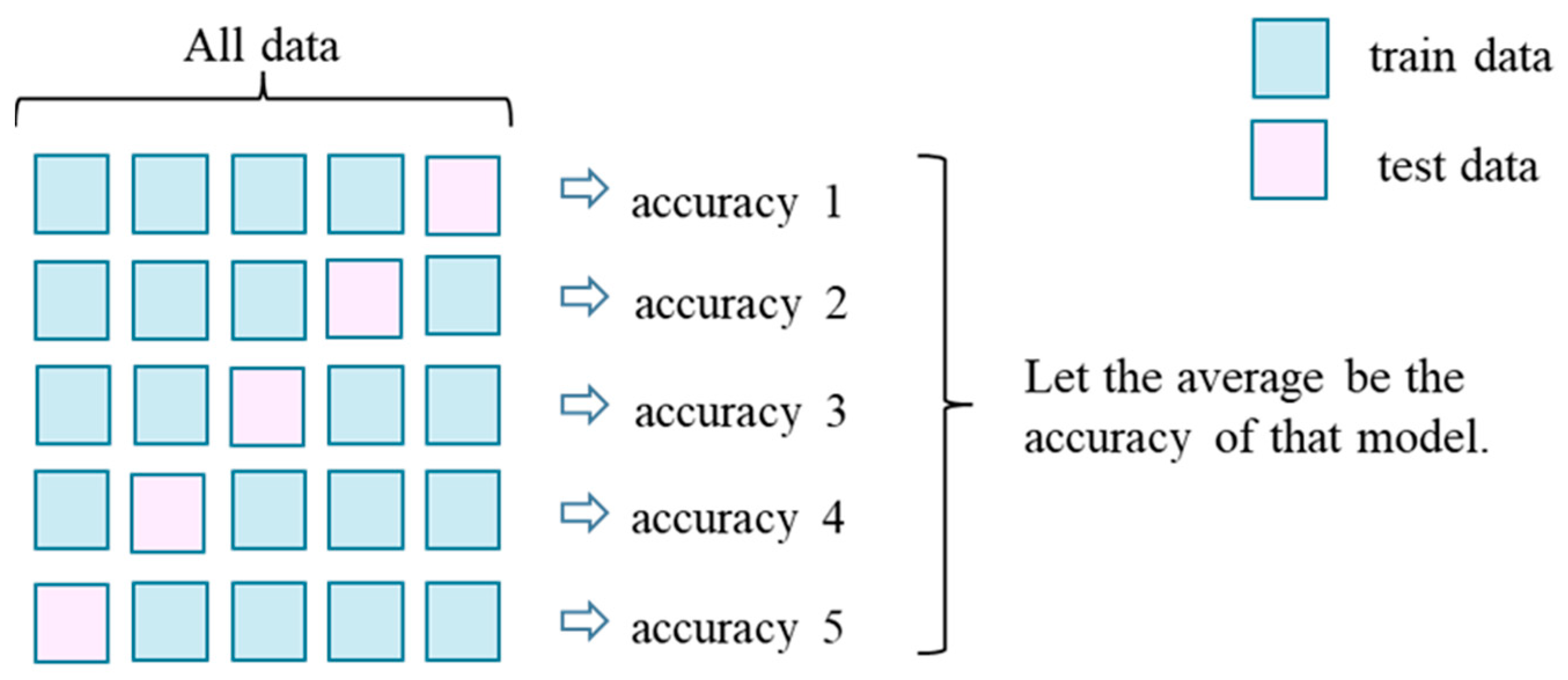
Figure 2. Conceptual diagram of margins and support vectors.

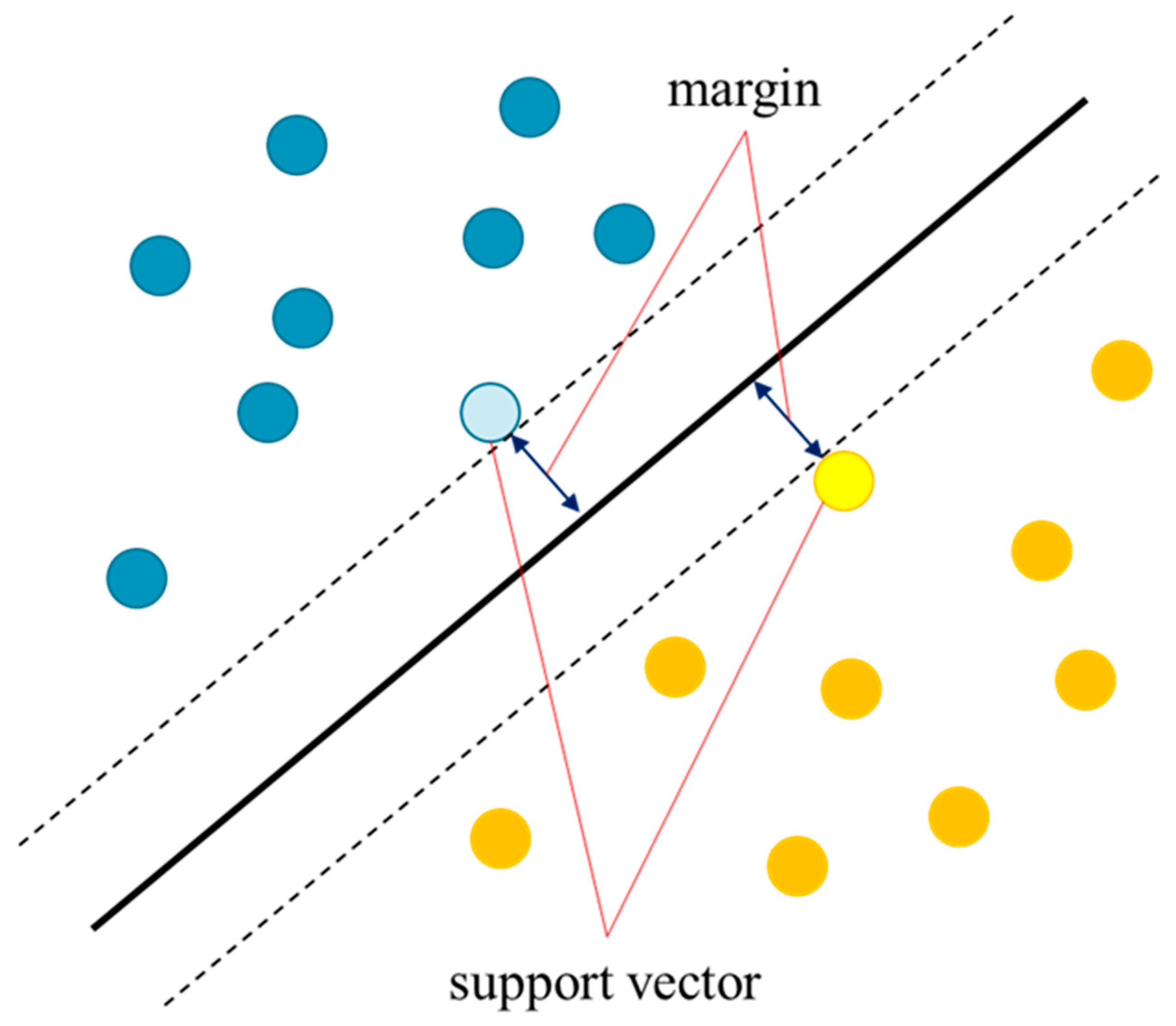
Figure 3. Conceptual diagram of the decision boundary for a change of C.

Figure 4. Conceptual diagram of the decision boundary in the change of gamma.

Figure 5. Overview of the DNN.

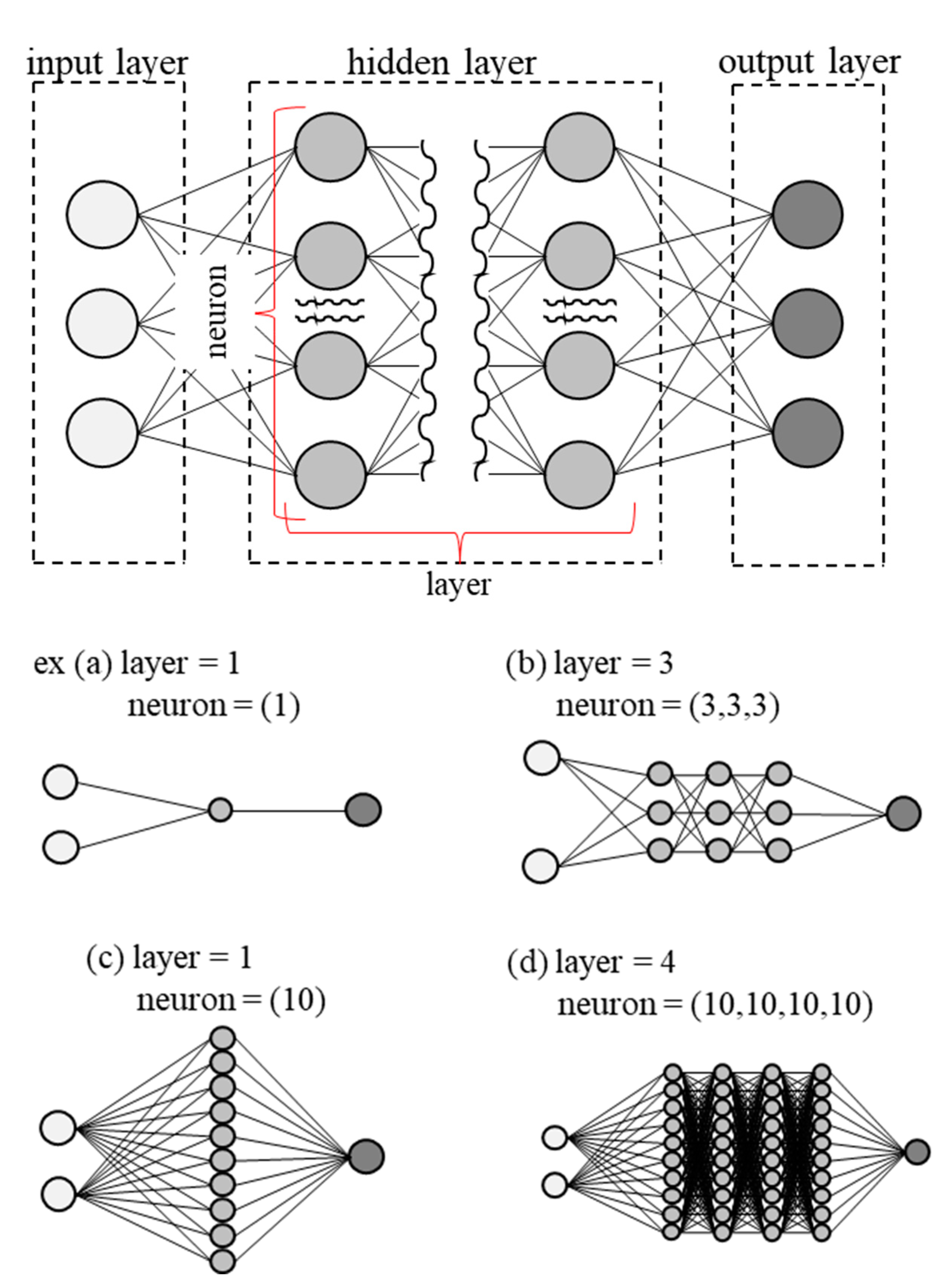
Figure 6. Photographs of the measuring equipment.

Figure 7. Distribution of occupants by gender and age in the winter poll.

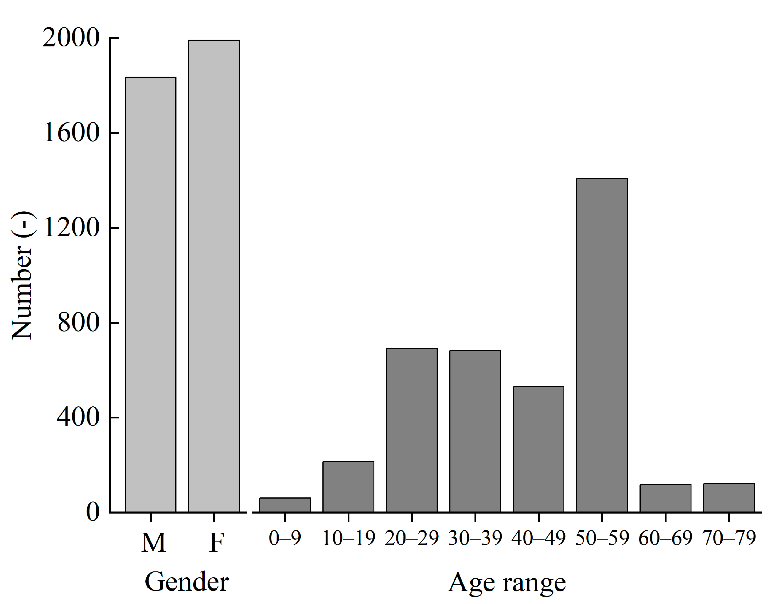
Figure 8. Outdoor air temperature trends in Gifu City from December 1, 2010, to February 28, 2011.

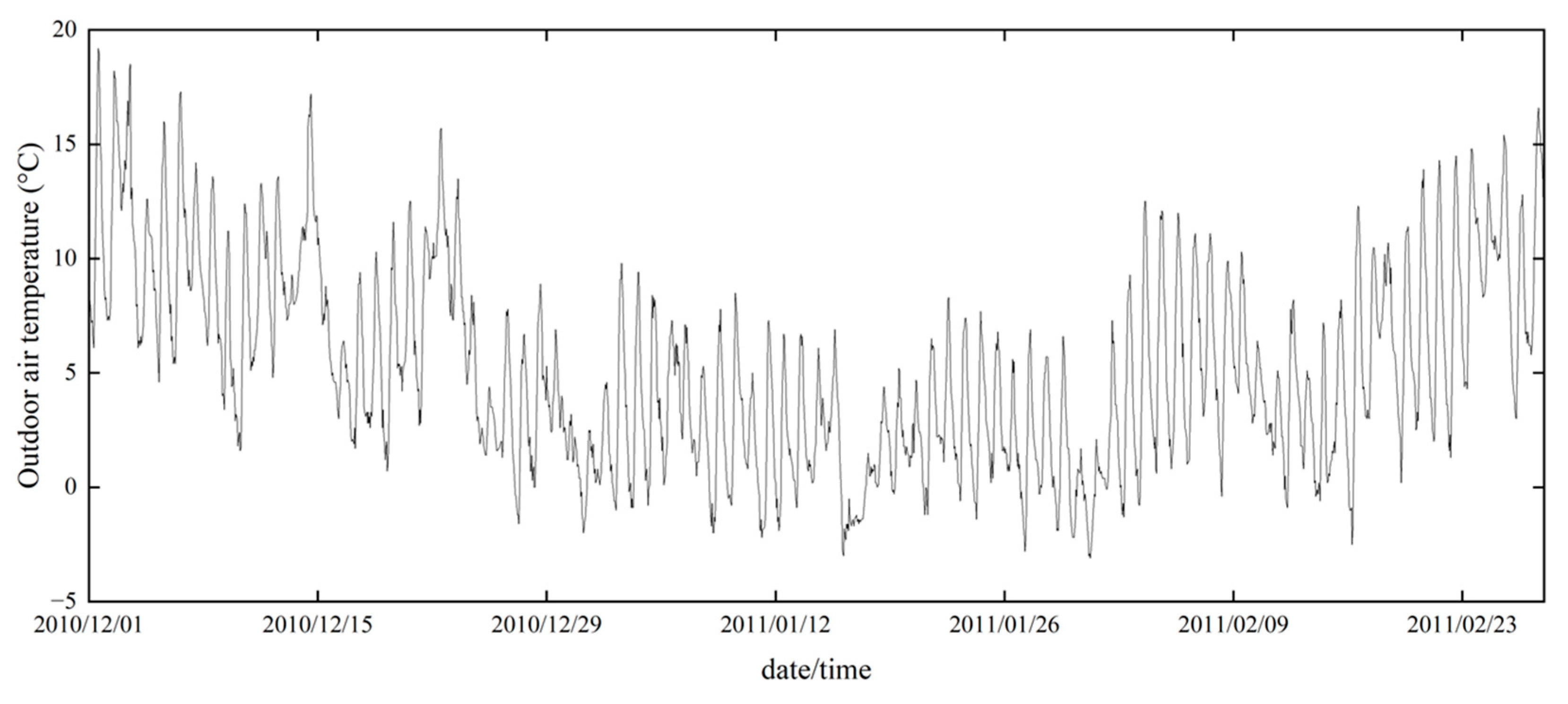
Figure 9. Variation of accuracy in the difference between C and gamma and variation of accuracy by response surface.

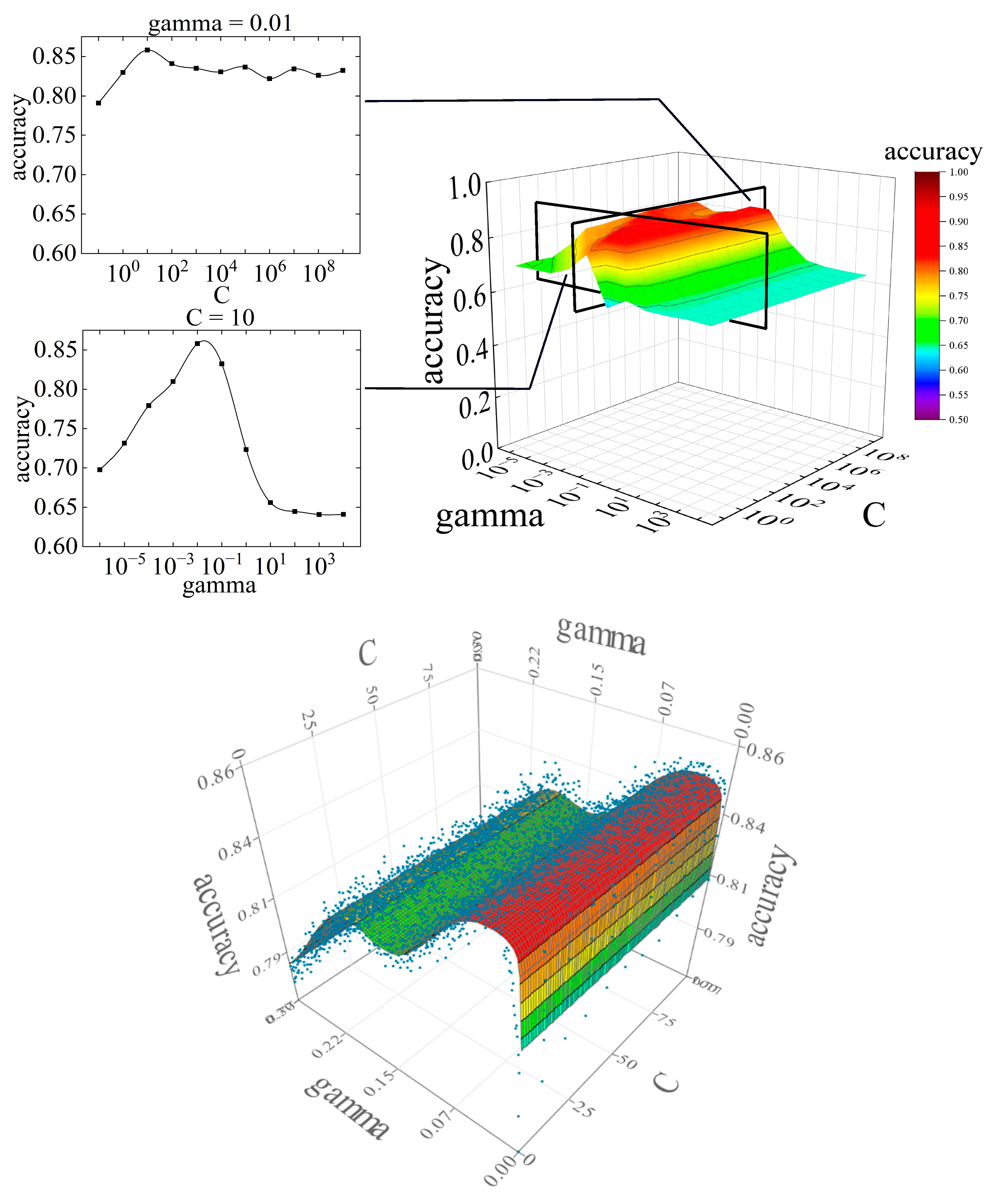
Figure 10. Relationship between C and accuracy at fixed gamma.

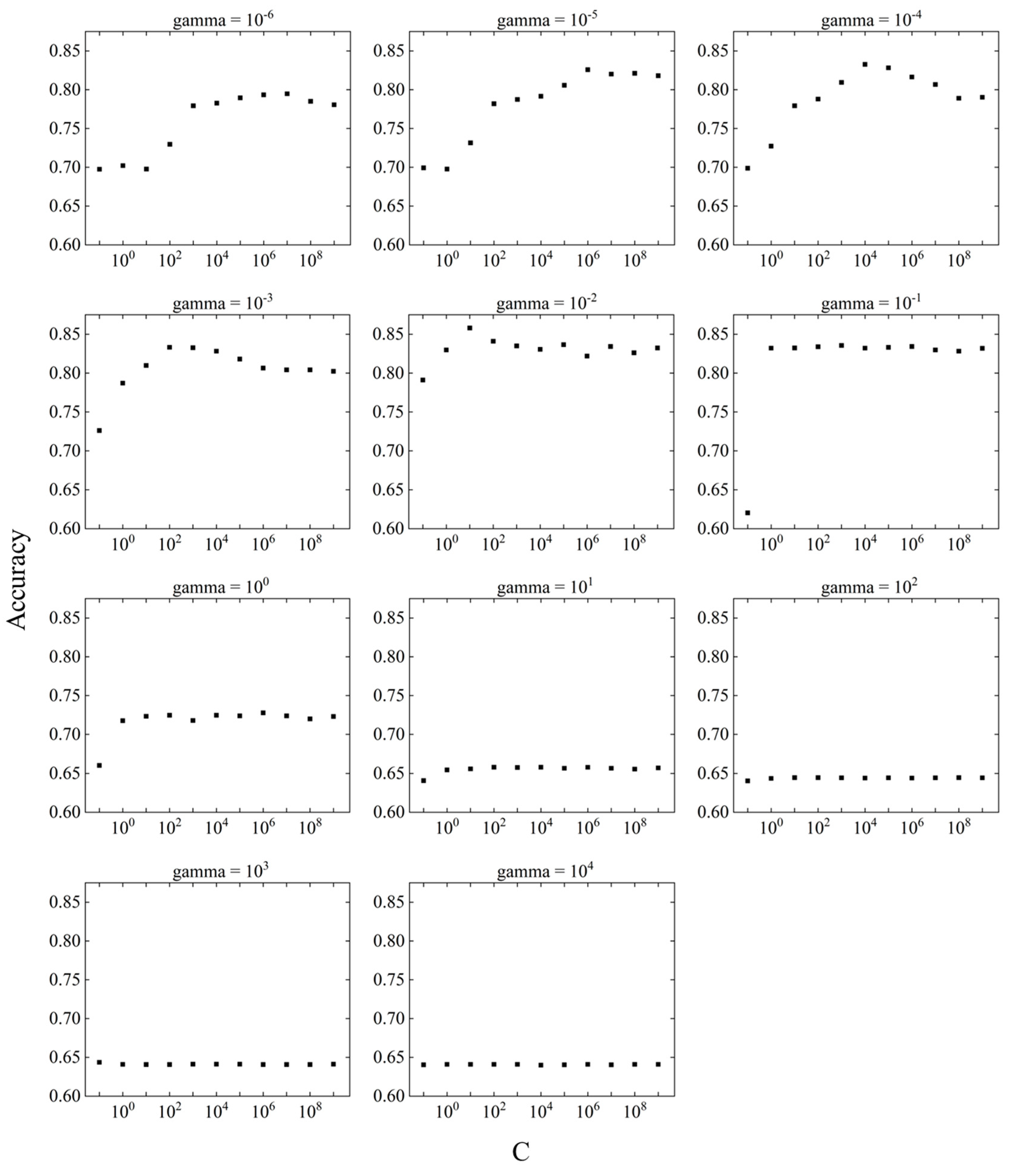
Figure 11. Relationship between gamma and accuracy at fixed C.

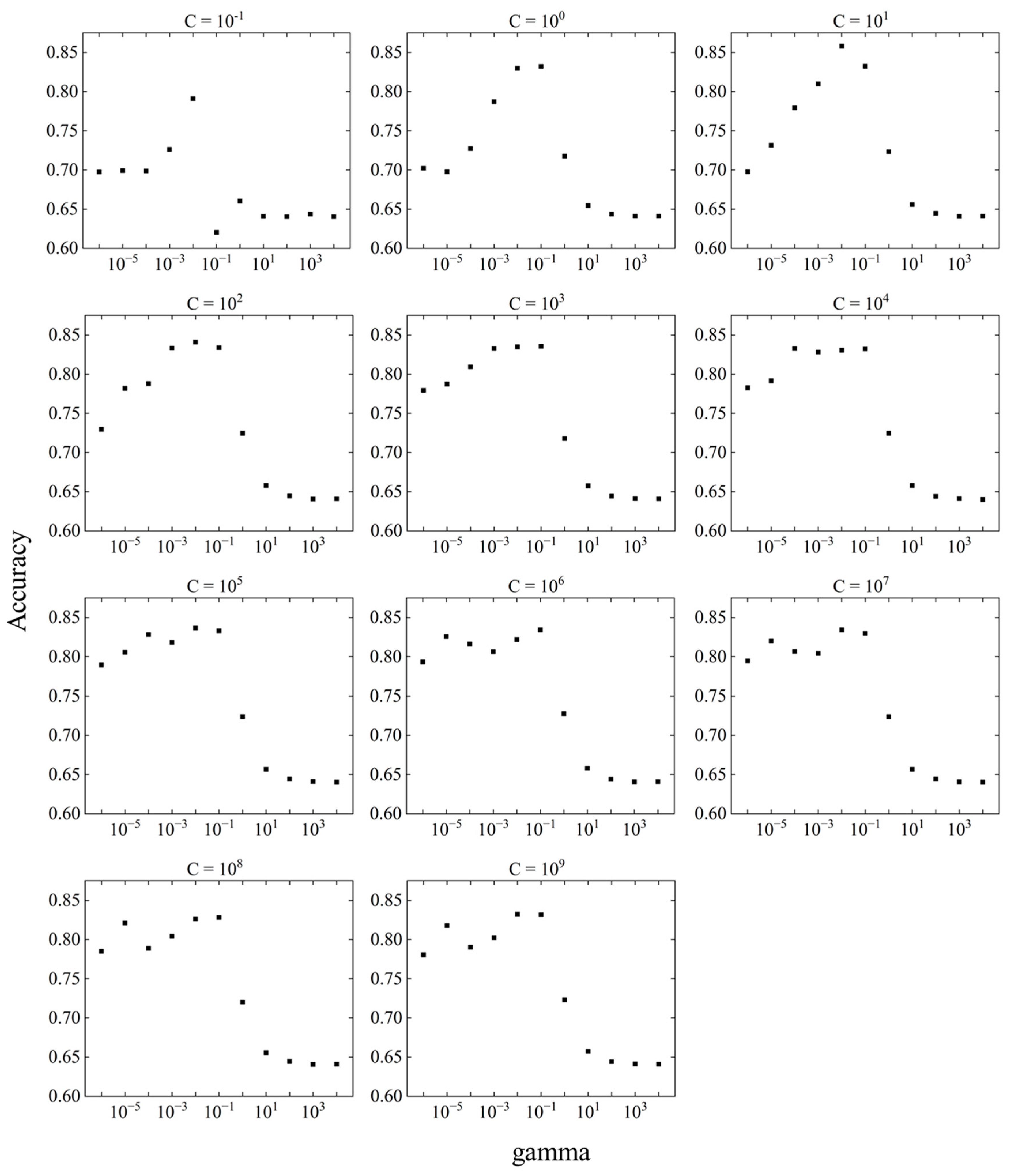
Figure 12. Relationship between gamma and accuracy at C = 10.

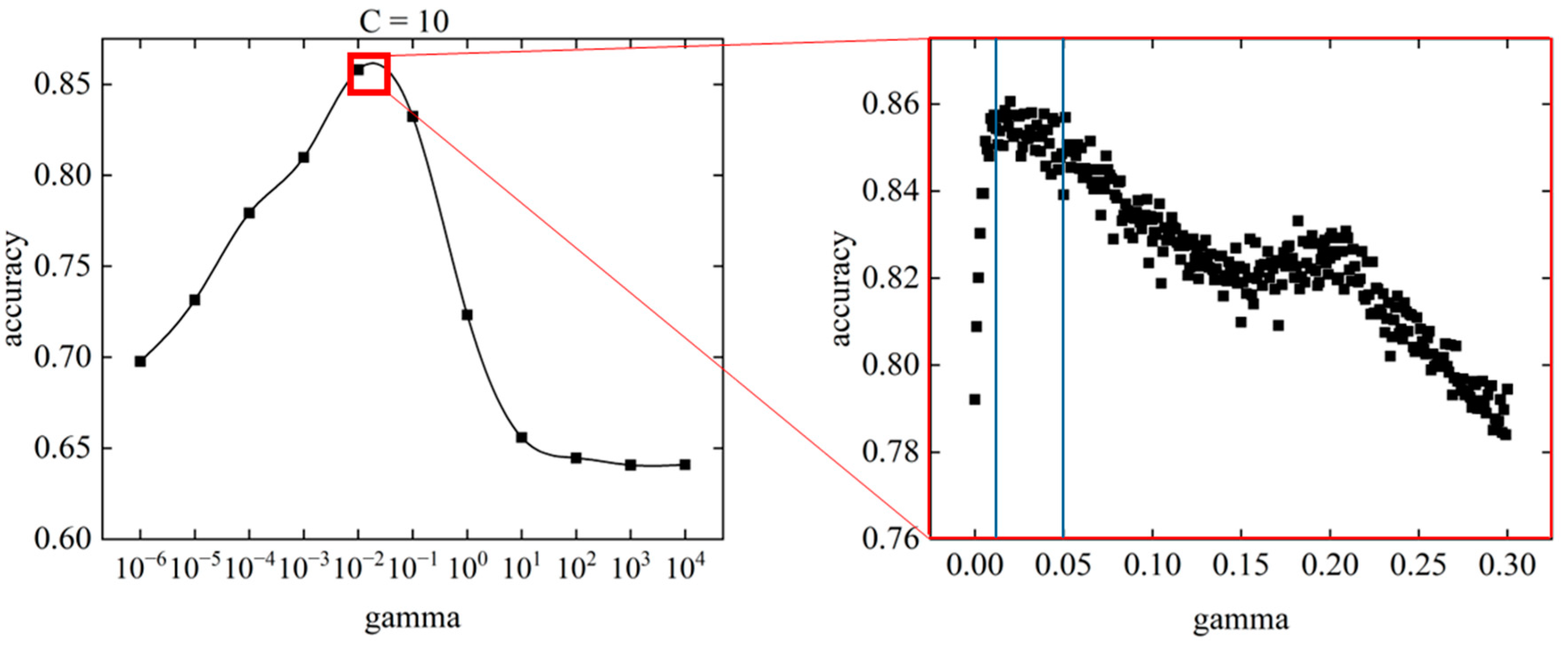
Figure 13. Variation of accuracy in the difference between layer and neuron and variation of accuracy by response surface.

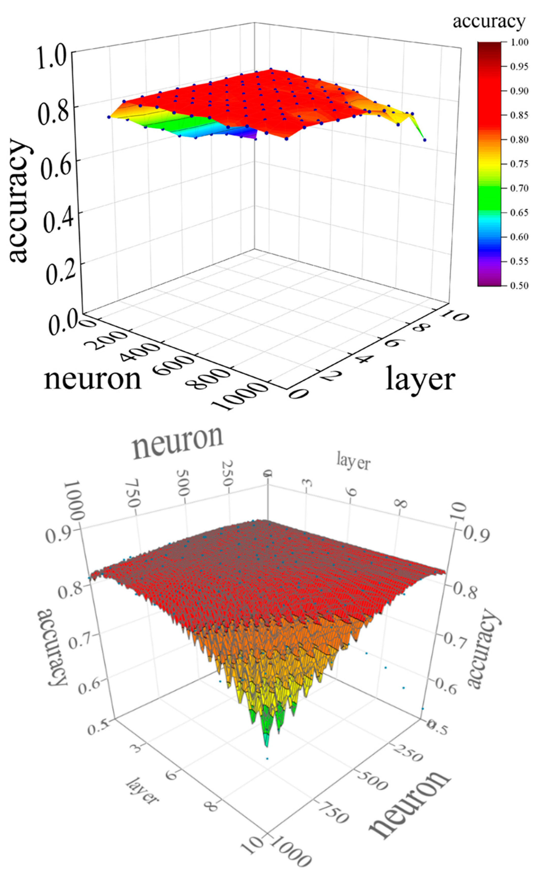
Figure 14. Layer and accuracy in neuron fixation.

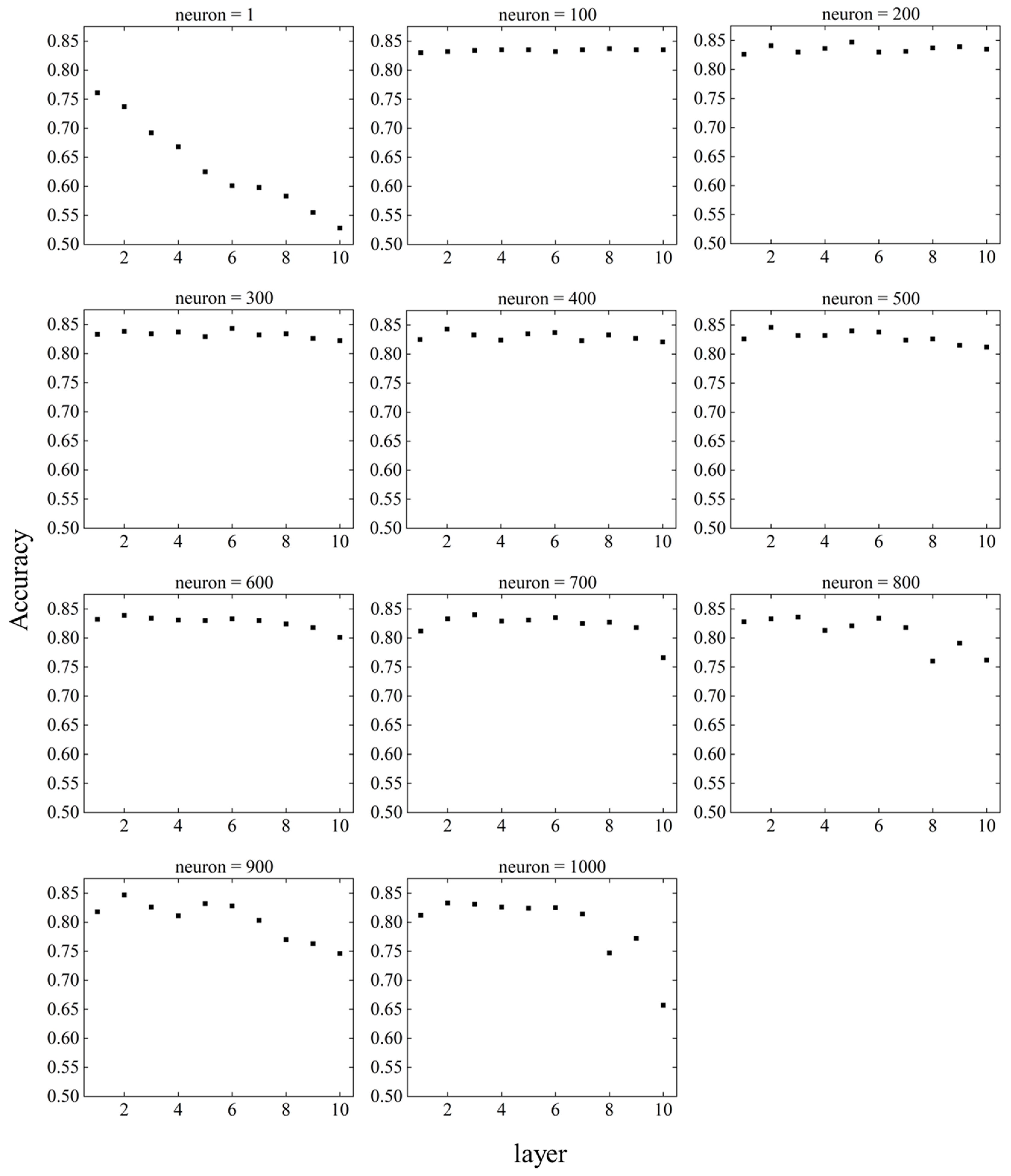
Figure 15. Neuron and accuracy in layer fixation.

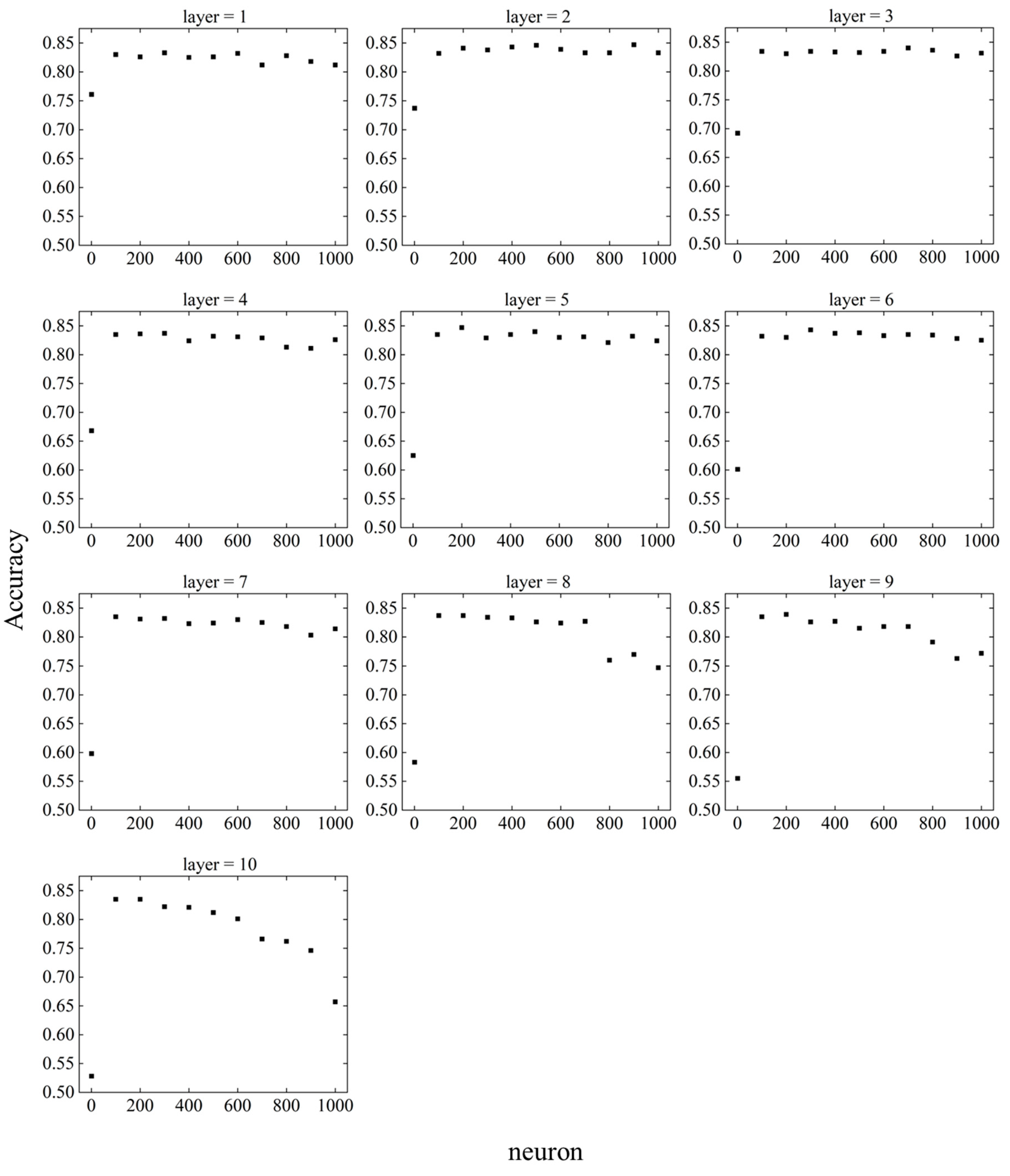
Figure 16. Time-series variation in forecast accuracy from day to day.

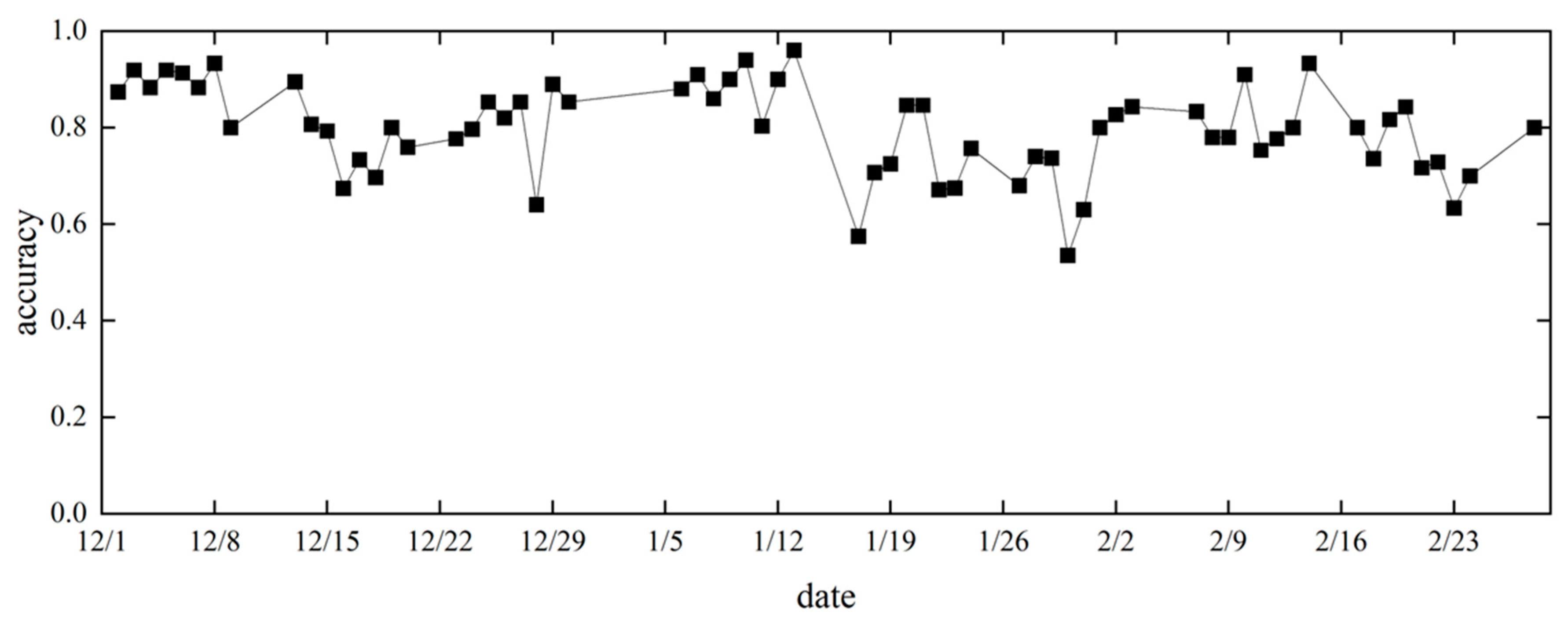
Figure 17. Number of data per day.

Figure 18. Time-series changes in forecast accuracy from week to week.

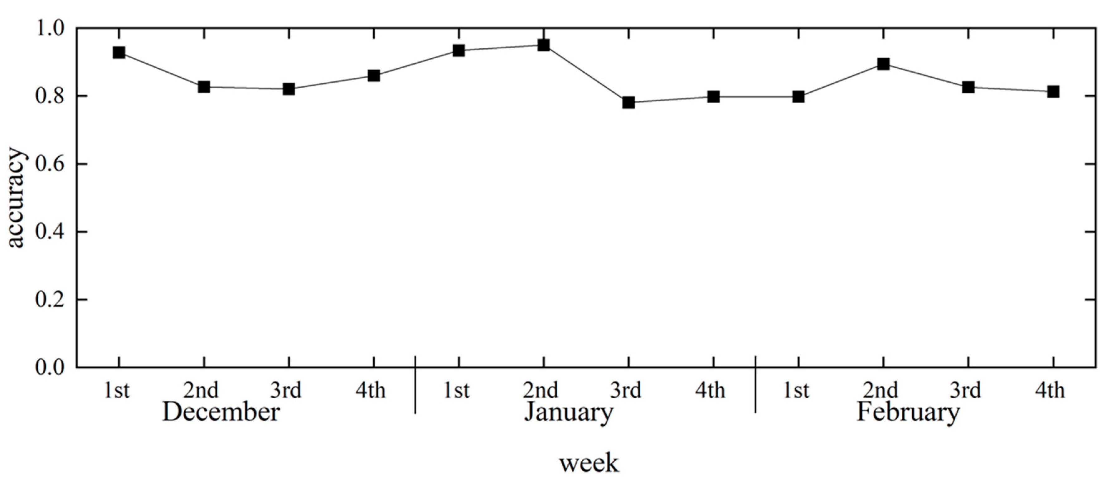
Figure 19. Number of data per week.

Table 1. Confusion matrix.

		Predicted Class
		Positive	Negative
Actual Class	Positive	True Positive (TP)	False Negative (FN)
Actual Class	Negative	False Positive (FP)	True Negative (TN)

Table 2. Gender and age distribution of survey participants.

Gender		Age group
Male	Female	0 – 9	10 – 19	20 – 29	30 – 39	40 – 49	50 – 59	60 – 69	70 – 79	80 +
32	33	2	3	13	12	8	23	2	2	0

Table 3. Summary of the measurement equipment.

Parameter	Instrument	Resolution	Accuracy	Manufacturer
Air temperature	Thermo Recorder TR-71	0.1 °C	±0.3 °C	T&D Corporation
Air temperature	Thermo Recorder TR-72	0.1 °C	±0.3 °C
Relative humidity	Thermo Recorder TR-72	1%	±5%
Globe temperature	Globe Thermometer 150 mm φ	–	–	SIBATA

Table 4. Statistical summary of thermal environment data and thermal comfort indices.

	Feature	Mean	Max.	Min.	Median	S.D.
Indoor	Air temperature (°C)	15.7	28.5	-0.5	16.5	4.65
	Relative humidity (%)	53.5	89	19	53	10.56
	Air velocity (m/s)	0.1	0.1	0.1	0.1	0.00
	Globe temperature (°C)	15.1	32.1	-1.6	15.8	4.55
	Wet-bulb temperature (°C)	10.6	19.9	-1.6	11.1	3.75
	Foot temperature (°C)	13.3	23.2	-0.5	13.8	3.84
Outdoor	Air temperature (°C)	4.7	18.5	-3.1	4	4.10
	Relative humidity (%)	66.0	91	15	68	15.64
	Air velocity (m/s)	2.4	10.9	0	1.9	1.61
	Atmospheric pressure (hPa)	1014.1	1025.2	997.9	1015.4	6.05
	Cloud cover (-)	6.9	10	0	9	3.79
	Precipitation (mm)	0.1	11.5	0	0	0.63
Thermal index	Operative temperature (°C)	15.4	29.1	-0.6	16.2	4.58
	MRT (°C)	15.1	32.1	-1.6	15.8	4.55
	Dew point temperature (°C)	6.0	18.1	-6.7	6.2	4.39
	WBGT (°C)	11.9	21.5	-1.3	12.6	3.93
	ET * (°C)	16.1	32.8	-0.5	16.6	5.00
	SET * (°C)	17.8	36.9	-3.9	17.9	6.69
	Neutral temperature (°C)	17.7	29.1	1.4	18.4	4.37
	Tdiff (°C)	-2.3	2	-8	-2	1.94
	T_op - 18 (°C)	-2.6	11.1	-18.6	-1.8	4.59
Human factor	Metabolic rate (met)	1.3	2	0.8	1.2	0.39
Human factor	Clothing insulation (clo)	0.8	2.7	0.3	0.7	0.32

MRT, mean radiant air temperature; WBGT, wet bulb globe temperature; ET*, new effective temperature; SET*, standard new effective temperature; Tdiff, difference between operative temperature and neutral temperature; T_op-18, difference between 18 °C and current T_op.

Table 5. Indoor environmental conditions in the poll during the period.

Occupant behavior	Number	On (Open)	Off (Close)
Heating	3821	2442	1379
Window	3821	112	3709
Door	3821	611	3210
Curtain	3821	1263	2558
Kotatsu	3821	1019	2802

Table 6. Statistical summary of subjective votes in the winter analysis.

Subjective vote	Proportion (%)
Thermal sensation	Cool	Neutral	Warm
Thermal sensation	32.0	68.0	0.0
Thermal conscious	Unconscious		Conscious
Thermal conscious	37.6		62.4
Thermal acceptability	Unacceptable		Acceptable
Thermal acceptability	12.3		87.7
Thermal tolerance	Intolerable		Tolerable
Thermal tolerance	9.7		90.3
Affective assessment	Uncomfortable		Comfortable
Affective assessment	18.9		81.1
Thermal preference	Cooler	No change	Warmer
Thermal preference	0.2	34.3	65.5

Table 7. Features used in the winter analysis.

		Features
Thermal environmental data	Indoor	Indoor air temperature, indoor relative humidity, indoor air velocity, globe temperature, wet-bulb temperature, foot temperature
Thermal environmental data	Outdoor	Outdoor air temperature, outdoor relative humidity, outdoor air velocity, atmospheric pressure, cloud cover, precipitation
Thermal comfort indices		Operative temperature, MRT, dew point temperature, WBGT, ET, SET, neutral temperature, Tdiff, T_op -18
Subjective vote		Thermal sensation, thermal conscious, thermal acceptability, thermal tolerance, Affective assessment, thermal preference
Human factor		Gender, age, metabolic rate, clothing insulation, posture
Occupant behavior		Window, door, curtain, kotatsu
Other		Date/time

Table 8. Comparison of accuracy of machine learning models as a function of initial conditions.

	Accuracy	Precision	Recall	F-measure
LR	0.783	0.862	0.787	0.823
SVM	0.770	0.829	0.807	0.818
DNN	0.827	0.882	0.843	0.862

Table 9. Comparison of the evaluation index by feature selection.

Models	Feature selection	Accuracy	Precision	Recall	F-measure
LR	FS	0.795	0.872	0.796	0.832
LR	BE	0.795	0.871	0.798	0.833
SVM	FS	0.793	0.810	0.884	0.845
SVM	BE	0.802	0.813	0.898	0.853
DNN	FS	0.843	0.891	0.860	0.875
DNN	BE	0.847	0.896	0.861	0.878

Table 10. Features selected for forward selection and backward elimination.

			LR		SVM		DNN
			FS	BE	FS	BE	FS	BE
Thermal environmental data	Indoor	Air temperature	0	0	0	0	1	1
		Relative humidity	1	0	1	1	1	1
		Air velocity	1	1	0	0	1	1
		Globe temperature	0	1	0	0	0	1
		Wet-bulb temperature	1	0	0	0	1	1
		Foot temperature	1	1	0	0	1	1
	Outdoor	Air temperature	1	1	1	1	1	1
		Relative humidity	1	0	1	0	0	0
		Air velocity	0	0	0	0	1	0
		Atmospheric pressure	1	0	1	0	1	1
		Cloud cover	0	1	0	0	0	0
		Precipitation	0	0	0	0	1	1
Thermal comfort indices		Operative temperature	1	0	0	0	1	0
		MRT	1	0	0	0	1	1
		Dew point temperature	0	1	0	1	0	1
		WBGT	1	0	0	0	1	1
		ET*	1	1	0	0	0	1
		SET*	0	1	0	0	0	1
		Neutral temperature	1	0	0	0	1	0
		Tdiff	0	1	0	0	0	1
		T_op-18	0	0	1	0	1	1
Subjective vote		Thermal sensation	1	1	1	1	1	1
		Thermal conscious	0	1	1	0	1	1
		Thermal acceptability	1	1	1	0	1	1
		Thermal tolerance	1	0	1	1	1	1
		Affective assessment	0	0	1	1	1	1
		Thermal preference	1	0	1	0	1	1
Human factor		Gender	0	0	1	0	1	1
		Age	1	1	1	1	1	1
		Metabolic rate	0	0	1	0	1	1
		Clothing insulation	0	0	0	0	0	1
		Posture	1	1	1	1	1	1
Occupant behavior		Window	1	1	1	1	1	1
		Door	1	1	1	1	1	1
		Curtain	0	0	1	1	1	1
		Kotatsu	1	1	1	1	1	1
Other		Date/Time	1	1	1	1	1	1

1 indicates that the feature was selected in FS and BE. 0 indicates that the feature was not selected in FS and BE.

Table 11. Comparison of indicators by linear regression.

			Coefficient	Std. Error	t-Stat	p-Value
Thermal environmental data	Indoor	Air temperature	0.362	0.002	235.1	0.000
		Relative humidity	0.012	0.001	20.7	0.000
		Air velocity	-0.001	NaN	NaN	NaN
		Globe temperature	0.083	0.002	54.8	0.000
		Wet-bulb temperature	-0.093	0.002	-48.6	0.000
		Foot temperature	-0.043	0.002	-25.7	0.000
	Outdoor	Air temperature	-0.036	0.002	-23.8	0.000
		Relative humidity	-0.001	0.000	-1.8	0.072
		Air velocity	0.008	0.004	2.1	0.038
		Atmospheric pressure	0.000	0.001	0.0	0.996
		Cloud cover	-0.001	0.002	-0.4	0.703
		Precipitation	0.013	0.010	1.4	0.175
Thermal comfort indices		Operative temperature	-0.143	0.002	-92.7	0.000
		MRT	0.083	0.002	54.4	0.000
		Dew point temperature	0.030	0.002	18.8	0.000
		WBGT	-0.036	0.002	-19.8	0.000
		ET*	-0.013	0.001	-9.1	0.000
		SET*	0.027	0.001	26.1	0.000
		Neutral temperature	-0.101	0.002	-67.2	0.000
		Tdiff	-0.044	0.003	-12.7	0.000
		T_op-18	-0.149	0.002	-96.7	0.000
Subjective vote		Thermal sensation	-0.022	0.007	-3.2	0.001
		Thermal conscious	-0.007	0.013	-0.6	0.560
		Thermal acceptability	0.033	0.019	1.7	0.087
		Thermal tolerance	0.118	0.022	5.4	0.000
		Affective assessment	0.008	0.008	1.0	0.305
		Thermal preference	0.022	0.013	1.6	0.100
Human factor		Gender	0.024	0.012	2.0	0.049
		Age	-0.003	0.000	-6.4	0.000
		Metabolic rate	-0.115	0.016	-7.2	0.000
		Clothing insulation	-0.255	0.019	-13.2	0.000
		Posture	-0.014	0.002	-6.4	0.000
Occupant behavior		Window	-0.269	0.037	-7.3	0.000
		Door	-0.204	0.017	-11.9	0.000
		Curtain	0.098	0.013	7.5	0.000
		Kotatsu	0.071	0.014	5.1	0.000
Intercept			-2.892	Infinity	0.0	1.000

Disclaimer/Publisher’s Note: The statements, opinions and data contained in all publications are solely those of the individual author(s) and contributor(s) and not of MDPI and/or the editor(s). MDPI and/or the editor(s) disclaim responsibility for any injury to people or property resulting from any ideas, methods, instructions or products referred to in the content.

© 2023 by the authors. Licensee MDPI, Basel, Switzerland. This article is an open access article distributed under the terms and conditions of the Creative Commons Attribution (CC BY) license (http://creativecommons.org/licenses/by/4.0/).

Copyright: This open access article is published under a Creative Commons CC BY 4.0 license, which permit the free download, distribution, and reuse, provided that the author and preprint are cited in any reuse.

MDPI Initiatives

Important Links

Choose an area of interest and we will send you notifications of new preprints at your preferred frequency.

Disclaimer