Submitted:
17 May 2023
Posted:
18 May 2023
You are already at the latest version
Abstract
Keywords:
1. Introduction
- In medical imaging, intrinsic and extrinsic factors cause an image’s resolution loss. The intrinsic limitation mainly originates from the physical limitations of imaging systems such as X-rays, MRIs, CTs, and ultrasounds. An imaging system’s spatial resolution is limited by factors such as the size of the detector or sensor, the wavelength of the imaging radiation, and the optics used to focus the radiation onto the detector. Extrinsic resolution limitations result from various factors during the image acquisition process, such as motion artifacts, patient movement, and image noise. SR technique can overcome extrinsic drawbacks.
- In the satellite field, the image captured can be affected by some natural conditions, such as haze, fog, and cloud cover. This impacts the quality and resolution of satellite images. These conditions can cause distortion, blurring, or loss of contrast in the images, affecting interpretation and analysis accuracy. Moreover, the system itself considerably contributes to the quality of the image. The size and design of the imaging sensor, the satellite’s altitude, and the imaging sensor’s angle are some factors that limit the ability to detect and identify small objects or features. SR helps recover important information, which can be used for image classification or image recognition of an area or geographical location.
- In the field of information transmission, because high-resolution images require more data to represent, transmitting or storing high-resolution images requires more bandwidth and storage space than lower-resolution ones. This can lead to network congestion and high latency, which negatively affect the user experience with phenomena like video lag or prolonged loading. SR can address this issue. Firstly, the image will be degraded in quality before being sent to the gateway. Secondly, the low-resolution image is processed into a high-quality image before being sent to the end-user device.
- Conduct a comprehensive survey of feasible solutions and optimization methods for SISR problems.
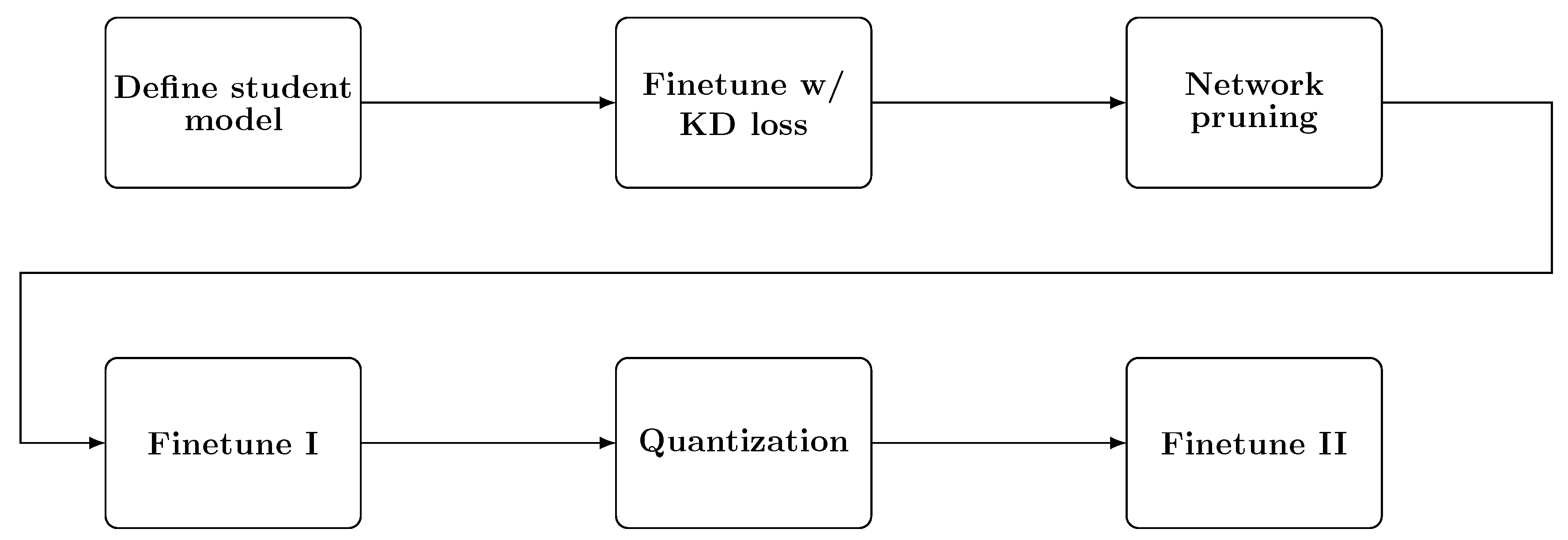
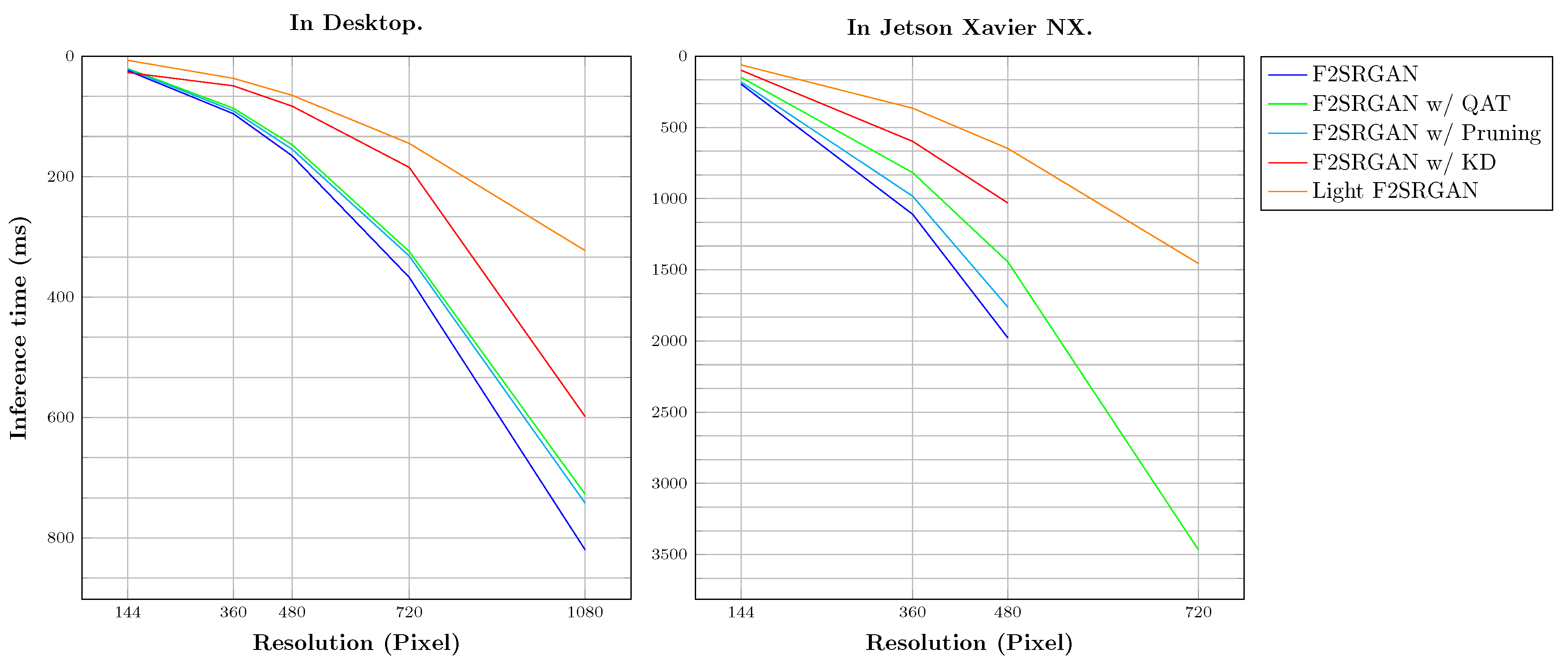
- Revisit the optimization methods to fit with our previous work F2SRGAN, a lightweight GAN-based perceptual-oriented SISR model [8] to reduce the inference time without significantly compromising the perceptual quality as a case study.
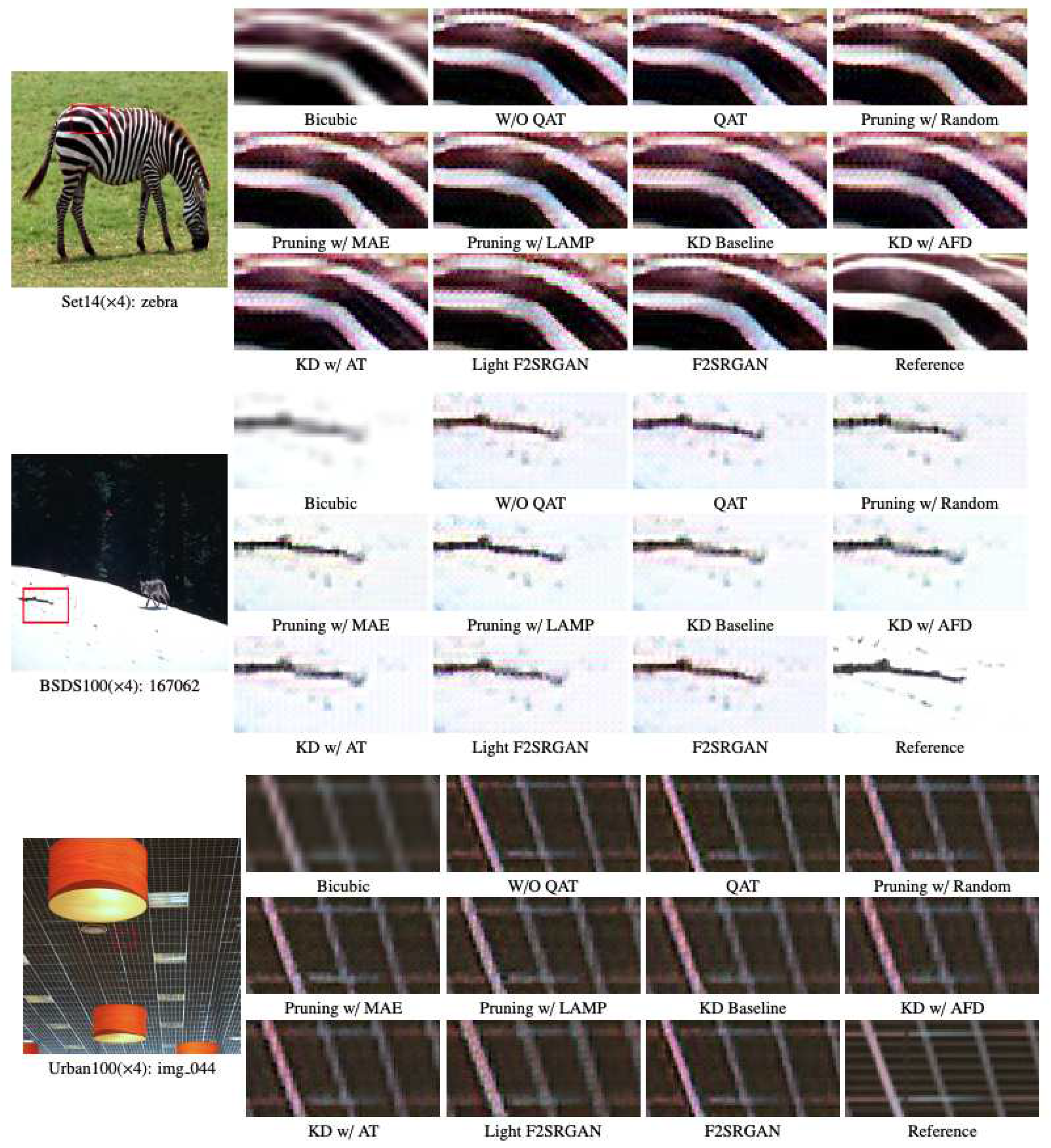
- Conduct in-depth experiments to prove the effectiveness of the proposed optimization pipeline.
2. Existing Approaches for Single-Image Super-Resolution (SISR)
2.1. Convolutional Neural Network (CNN) based methods
2.2. Distillation method
2.3. Attention-based method
2.4. Feedback network-based methods
2.5. Recursive learning-based methods
2.6. GAN-based methods
2.7. Transformer-based methods
2.8. Frequency-domain based methods
3. Optimization Techniques for SISR Problems
3.1. Quantization
- Stage 1: Train the network with floating-point operations.
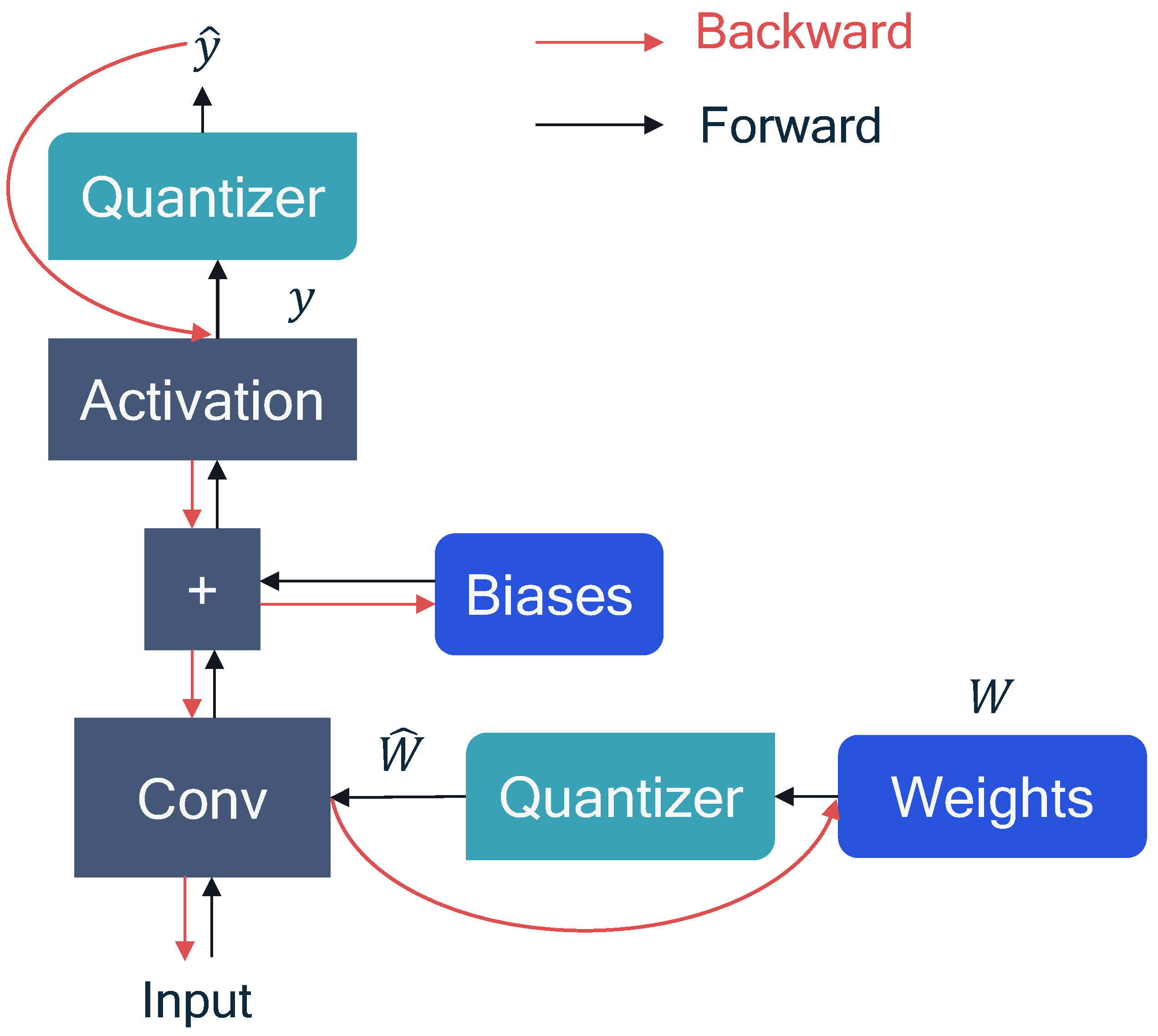
- Stage 2: Insert Fake quantization layers into the trained network. The layer is used to simulate the process of integer quantization using floating-point computations. It is usually performed by a quantization step (Q) followed by a dequantization step (DQ).
- Stage 3: Perform fine-tuning of the model. Note that in this process, the gradient is still used in floating-point.
- Stage 4: Perform execution by removing and loading the quantized weights.
3.2. Network pruning
3.3. Knowledge distillation
4. A Case Study
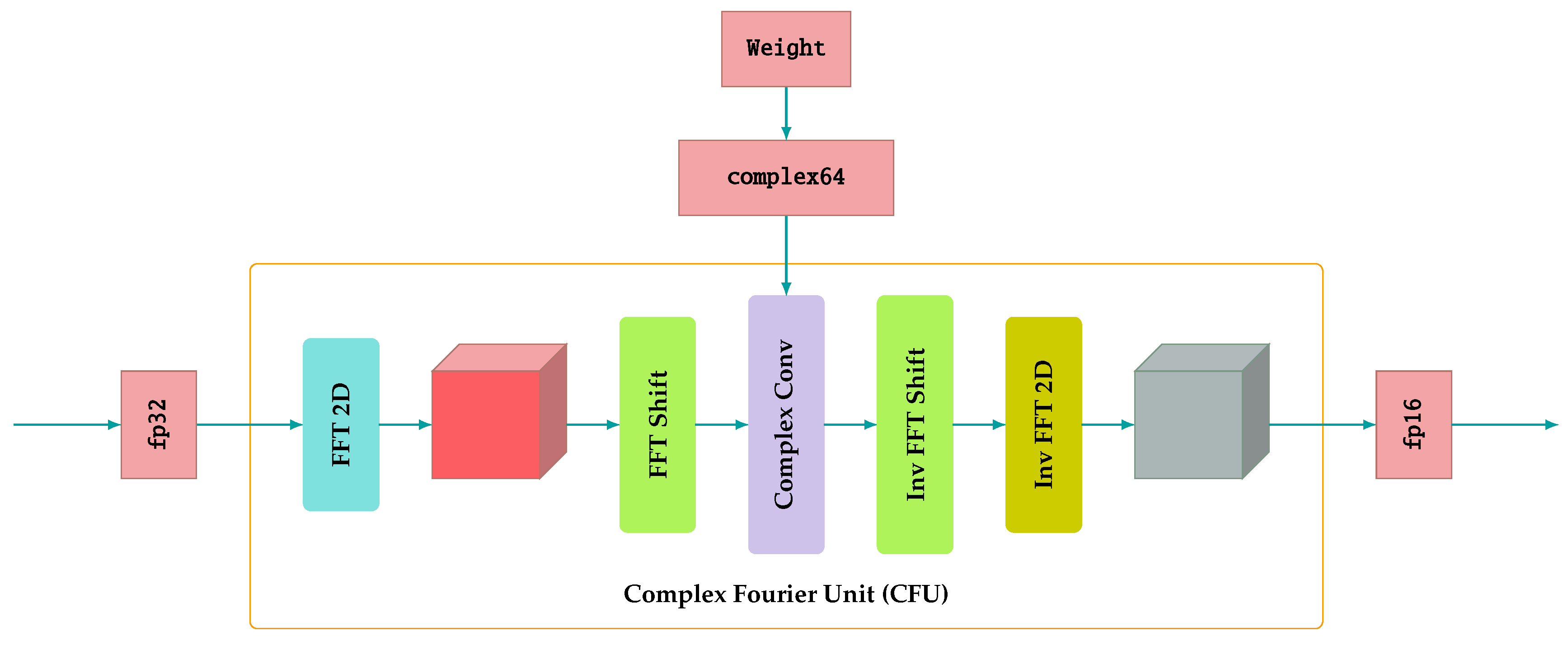
4.1. Quantization
4.2. Network pruning
- Random: Randomize the importance score of parameters within each group.
- LAMP: Conceptually, LAMP measures the importance of a connection with the unpruned ones. LAMP considers network layers as operators, following the logic of lookahead pruning [61]. Based on minimizing model-level distortion, Lee et al. [62] propose a score function. First, the author sorts the weight tensor in ascending order so that for any pair of u and v with , the connected weights maintain at least the same inequality . The LAMP score is calculated using Eq. (16).where W is weight tensor and u the index of calculated weight. The score function guarantees that only one weight in each layer has a score of 1, which is the highest magnitude.
4.3. Knowledge distillation
- Activation-based and Gradient-based Attention Transfer: Attention Transfer (AT) distillation is proposed by Sergey Zagoruyko et al. [63] with the use of attention maps, which can be formulated by (17):where is the indices of all Student-Teacher attention maps pair, represents the aggregated feature map in space with normalization, which means that we replace each vectorized attention map with .
- Attention-based Feature Distillation: Attention-based Feature Distillation is proposed by Mingi Ji et al. [64] to define hint position and weights for hints. The author evaluates the pair of features between Student and Teacher through attention values. The loss component can be presented by (18):where according to the author, represents the normalized channel-wise average pooling function with normalization. is the up-sampled or down-sampled version of to match the feature map size of the Teacher model.
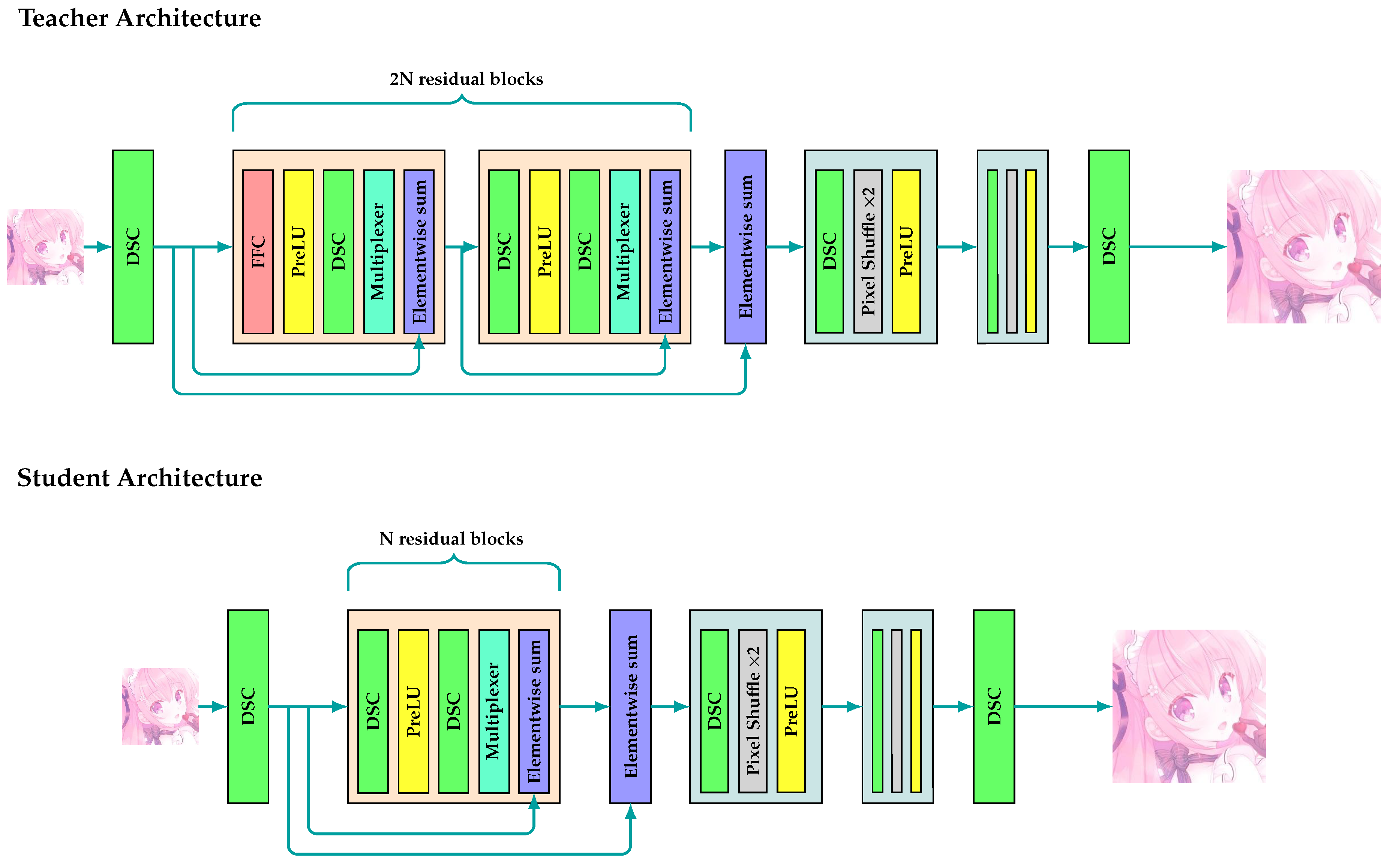
4.4. Light F2SRGAN
5. Experiments
5.1. Datasets
5.2. Implementation Details
5.3. Evaluation Metrics
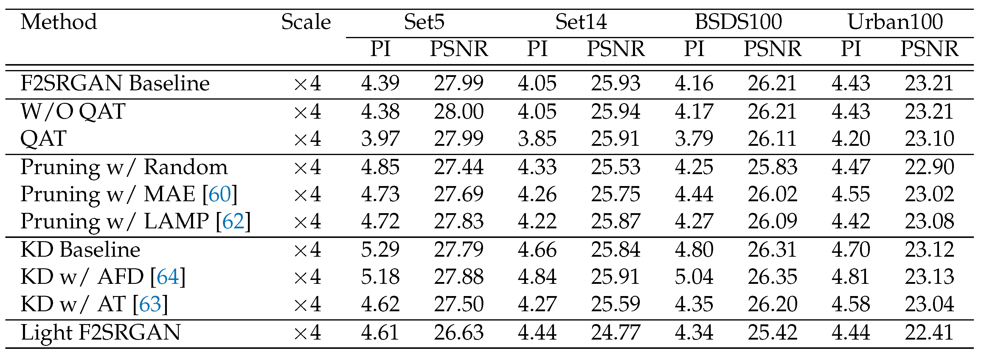
5.4. Experimental Results
 |
6. Conclusions
Author Contributions
Funding
Acknowledgments
Conflicts of Interest
References
- Park, J.; Hwang, D.; Kim, K.Y.; Kang, S.K.; Kim, Y.K.; Lee, J.S. Computed tomography super-resolution using deep convolutional neural network. Physics in Medicine & Biology 2018, 63, 145011. [CrossRef]
- You, C.; Li, G.; Zhang, Y.; Zhang, X.; Shan, H.; Li, M.; Ju, S.; Zhao, Z.; Zhang, Z.; Cong, W.; others. CT Super-resolution GAN Constrained by the Identical, Residual, and Cycle Learning Ensemble (GAN-CIRCLE). IEEE Transactions on Medical Imaging 2019, 39, 188–203. [CrossRef]
- Chen, Y.; Xie, Y.; Zhou, Z.; Shi, F.; Christodoulou, A.G.; Li, D. Brain MRI super resolution using 3D deep densely connected neural networks. 15th International Symposium on Biomedical Imaging (ISBI 2018). IEEE, 2018, pp. 739–742. [CrossRef]
- Müller, M.U.; Ekhtiari, N.; Almeida, R.M.; Rieke, C. Super-resolution of multispectral satellite images using convolutional neural networks. arXiv preprint arXiv:2002.00580 2020.
- Shermeyer, J.; Van Etten, A. The Effects of Super-Resolution on Object Detection Performance in Satellite Imagery. IEEE/CVF Conference on Computer Vision and Pattern Recognition Workshops (CVPRW), 2019, pp. 1432–1441. [CrossRef]
- Kwon, I.; Li, J.; Prasad, M. Lightweight Video Super-Resolution for Compressed Video. Electronics 2023, 12, 660. [CrossRef]
- Khani, M.; Sivaraman, V.; Alizadeh, M. Efficient Video Compression via Content-Adaptive Super-Resolution. IEEE/CVF International Conference on Computer Vision (ICCV), 2021, pp. 4521–4530. [CrossRef]
- Nguyen, D.P.; Vu, K.H.; Nguyen, D.D.; Pham, H.A. F2SRGAN: A Lightweight Approach Boosting Perceptual Quality in Single Image Super-Resolution via a Revised Fast Fourier Convolution. IEEE Access 2023, 11, 29062–29073. [CrossRef]
- Dong, C.; Loy, C.C.; He, K.; Tang, X. Image Super-Resolution Using Deep Convolutional Networks. CoRR 2015, abs/1501.00092. [CrossRef]
- Ahn, S.; Kang, S.J. Deep Learning-based Real-Time Super-Resolution Architecture Design. Journal of Broadcast Engineering 2021, 26, 167–174. [CrossRef]
- Lai, W.; Huang, J.; Ahuja, N.; Yang, M. Deep Laplacian Pyramid Networks for Fast and Accurate Super-Resolution. CoRR 2017, abs/1704.03915. [CrossRef]
- Hui, Z.; Wang, X.; Gao, X. Fast and Accurate Single Image Super-Resolution via Information Distillation Network. CoRR 2018, abs/1803.09454. [CrossRef]
- Hui, Z.; Gao, X.; Yang, Y.; Wang, X. Lightweight Image Super-Resolution with Information Multi-distillation Network. 27th ACM International Conference on Multimedia. ACM, 2019, p. 2024–2032. [CrossRef]
- Hu, J.; Shen, L.; Sun, G. Squeeze-and-Excitation Networks. 2018 IEEE/CVF Conference on Computer Vision and Pattern Recognition, 2018, pp. 7132–7141. [CrossRef]
- Zhang, Y.; Li, K.; Li, K.; Wang, L.; Zhong, B.; Fu, Y. Image Super-Resolution Using Very Deep Residual Channel Attention Networks. CoRR 2018, abs/1807.02758. [CrossRef]
- Anwar, S.; Barnes, N. Densely Residual Laplacian Super-Resolution, 2019. [CrossRef]
- Niu, B.; Wen, W.; Ren, W.; Zhang, X.; Yang, L.; Wang, S.; Zhang, K.; Cao, X.; Shen, H. Single Image Super-Resolution via a Holistic Attention Network, 2020. [CrossRef]
- Haris, M.; Shakhnarovich, G.; Ukita, N. Deep Back-Projection Networks For Super-Resolution, 2018. [CrossRef]
- Li, Z.; Yang, J.; Liu, Z.; Yang, X.; Jeon, G.; Wu, W. Feedback Network for Image Super-Resolution, 2019. [CrossRef]
- Li, Q.; Li, Z.; Lu, L.; Jeon, G.; Liu, K.; Yang, X. Gated Multiple Feedback Network for Image Super-Resolution, 2019. [CrossRef]
- Liu, Z.S.; Wang, L.W.; Li, C.T.; Siu, W.C. Hierarchical Back Projection Network for Image Super-Resolution. 2019 IEEE/CVF Conference on Computer Vision and Pattern Recognition Workshops (CVPRW), 2019, pp. 2041–2050. [CrossRef]
- Liu, Z.S.; Wang, L.W.; Li, C.T.; Siu, W.C.; Chan, Y.L. Image Super-Resolution via Attention based Back Projection Networks, 2019, [arXiv:eess.IV/1910.04476].
- Ahn, N.; Kang, B.; Sohn, K. Fast, Accurate, and, Lightweight Super-Resolution with Cascading Residual Network. CoRR 2018, abs/1803.08664. [CrossRef]
- Choi, J.; Kim, J.; Cheon, M.; Lee, J. Lightweight and Efficient Image Super-Resolution with Block State-based Recursive Network. CoRR 2018, abs/1811.12546. [CrossRef]
- Li, J.; Yuan, Y.; Mei, K.; Fang, F. Lightweight and Accurate Recursive Fractal Network for Image Super-Resolution. 2019 IEEE/CVF International Conference on Computer Vision Workshop (ICCVW), 2019, pp. 3814–3823. [CrossRef]
- Cai, J.; Zeng, H.; Yong, H.; Cao, Z.; Zhang, L. Toward Real-World Single Image Super-Resolution: A New Benchmark and A New Model. CoRR 2019, abs/1904.00523. [CrossRef]
- Ledig, C.; Theis, L.; Huszar, F.; Caballero, J.; Cunningham, A.; Acosta, A.; Aitken, A.; Tejani, A.; Totz, J.; Wang, Z.; Shi, W. Photo-Realistic Single Image Super-Resolution Using a Generative Adversarial Network. IEEE Conference on Computer Vision and Pattern Recognition (CVPR). IEEE Computer Society, 2017, pp. 105–114. [CrossRef]
- Wang, X.; Yu, K.; Wu, S.; Gu, J.; Liu, Y.; Dong, C.; Qiao, Y.; Loy, C.C. ESRGAN: Enhanced Super-Resolution Generative Adversarial Networks. European Conference on Computer Vision (ECCV) Workshop. Springer International Publishing, 2019, pp. 63–79. [CrossRef]
- Krishnan, K.S.; Krishnan, K.S. SwiftSRGAN - Rethinking Super-Resolution for Efficient and Real-time Inference. 2021 International Conference on Intelligent Cybernetics Technology & Applications (ICICyTA), 2021, pp. 46–51. [CrossRef]
- Mirchandani, K.; Chordiya, K. DPSRGAN: Dilation Patch Super-Resolution Generative Adversarial Networks. 6th International Conference for Convergence in Technology (I2CT), 2021, pp. 1–7. [CrossRef]
- Zhang, K.; Liang, J.; Van Gool, L.; Timofte, R. Designing a Practical Degradation Model for Deep Blind Image Super-Resolution, 2021. [CrossRef]
- Lu, Z.; Liu, H.; Li, J.; Zhang, L. Efficient Transformer for Single Image Super-Resolution. CoRR 2021, abs/2108.11084. [CrossRef]
- Zhang, D.; Huang, F.; Liu, S.; Wang, X.; Jin, Z. SwinFIR: Revisiting the SwinIR with Fast Fourier Convolution and Improved Training for Image Super-Resolution, 2022. [CrossRef]
- Liang, J.; Cao, J.; Sun, G.; Zhang, K.; Van Gool, L.; Timofte, R. SwinIR: Image Restoration Using Swin Transformer. 2021 IEEE/CVF International Conference on Computer Vision Workshops (ICCVW), 2021, pp. 1833–1844. [CrossRef]
- Tsai, R. Multiframe Image Restoration and Registration. Advance Computer Visual and Image Processing 1984, 1, 317–339.
- Lee, J.; Jin, K.H. Local Texture Estimator for Implicit Representation Function. 2022 IEEE/CVF Conference on Computer Vision and Pattern Recognition (CVPR), 2022, pp. 1919–1928. [CrossRef]
- Zhang, K.; Gu, S.; Timofte, R.; Hui, Z.; Wang, X.; Gao, X.; Xiong, D.; Liu, S.; Gang, R.; Nan, N.; Li, C.; Zou, X.; Kang, N.; Wang, Z.; Xu, H.; Wang, C.; Li, Z.; Wang, L.; Shi, J.; Sun, W.; Lang, Z.; Nie, J.; Wei, W.; Zhang, L.; Niu, Y.; Zhuo, P.; Kong, X.; Sun, L.; Wang, W. AIM 2019 Challenge on Constrained Super-Resolution: Methods and Results, 2019. [CrossRef]
- Kim, J.; Lee, J.K.; Lee, K.M. Accurate Image Super-Resolution Using Very Deep Convolutional Networks. CoRR 2015, abs/1511.04587, [1511.04587].
- Xie, C.; Zeng, W.; Jiang, S.; Lu, X. Bidirectionally aligned sparse representation for single image super-resolution. Multimedia Tools and Applications 2018, 77, 7883–7907.
- Yang, C.; Lu, G. Deeply Recursive Low- and High-Frequency Fusing Networks for Single Image Super-Resolution. Sensors 2020, 20. [CrossRef]
- Goodfellow, I.; Pouget-Abadie, J.; Mirza, M.; Xu, B.; Warde-Farley, D.; Ozair, S.; Courville, A.; Bengio, Y. Generative Adversarial Networks. Commun. ACM 2020, 63, 139–144. [CrossRef]
- Wang, X.; Xie, L.; Dong, C.; Shan, Y. Real-ESRGAN: Training Real-World Blind Super-Resolution with Pure Synthetic Data. IEEE/CVF International Conference on Computer Vision Workshops (ICCVW), 2021, pp. 1905–1914. [CrossRef]
- Rahaman, N.; Baratin, A.; Arpit, D.; Draxler, F.; Lin, M.; Hamprecht, F.; Bengio, Y.; Courville, A. On the Spectral Bias of Neural Networks. 36th International Conference on Machine Learning. PMLR, 2019, pp. 5301–5310.
- Tancik, M.; Srinivasan, P.P.; Mildenhall, B.; Fridovich-Keil, S.; Raghavan, N.; Singhal, U.; Ramamoorthi, R.; Barron, J.T.; Ng, R. Fourier Features Let Networks Learn High Frequency Functions in Low Dimensional Domains. 34th International Conference on Neural Information Processing Systems. Curran Associates Inc., 2020, NIPS’20, pp. 7537––7547.
- Chi, L.; Jiang, B.; Mu, Y. Fast Fourier Convolution. Advances in Neural Information Processing Systems; Larochelle, H.; Ranzato, M.; Hadsell, R.; Balcan, M.; Lin, H., Eds. Curran Associates, Inc., 2020, Vol. 33, pp. 4479–4488.
- Jacob, B.; Kligys, S.; Chen, B.; Zhu, M.; Tang, M.; Howard, A.; Adam, H.; Kalenichenko, D. Quantization and Training of Neural Networks for Efficient Integer-Arithmetic-Only Inference. IEEE/CVF Conference on Computer Vision and Pattern Recognition (CVPR), 2018, pp. 2704–2713. [CrossRef]
- Bengio, Y.; Léonard, N.; Courville, A.C. Estimating or Propagating Gradients Through Stochastic Neurons for Conditional Computation. CoRR 2013, abs/1308.3432. [CrossRef]
- Siddegowda, S.; Fournarakis, M.; Nagel, M.; Blankevoort, T.; Patel, C.; Khobare, A. Neural Network Quantization with AI Model Efficiency Toolkit (AIMET). CoRR 2022, abs/2201.08442. [CrossRef]
- LeCun, Y.; Denker, J.; Solla, S. Optimal Brain Damage. Advances in Neural Information Processing Systems, 1989, Vol. 2.
- Zhang, Y.; Wang, H.; Qin, C.; Fu, Y. Learning Efficient Image Super-Resolution Networks via Structure-Regularized Pruning. International Conference on Learning Representations (ICLR), 2022.
- Yuan, M.; Lin, Y. Model Selection and Estimation in Regression with Grouped Variables. Journal of the Royal Statistical Society: Series B (Statistical Methodology) 2006, 68, 49–67. [CrossRef]
- Fang, G.; Ma, X.; Song, M.; Mi, M.B.; Wang, X. Depgraph: Towards Any Structural Pruning. arXiv:2301.12900 2023. [CrossRef]
- Buciluundefined, C.; Caruana, R.; Niculescu-Mizil, A. Model Compression. 12th ACM SIGKDD International Conference on Knowledge Discovery and Data Mining. ACM, 2006, p. 535–541. [CrossRef]
- Kim, T.; Oh, J.; Kim, N.Y.; Cho, S.; Yun, S.Y. Comparing Kullback-Leibler Divergence and Mean Squared Error Loss in Knowledge Distillation. Thirtieth International Joint Conference on Artificial Intelligence, (IJCAI), 2021, pp. 2628–2635. [CrossRef]
- Hinton, G.; Vinyals, O.; Dean, J. Distilling the Knowledge in a Neural Network. arXiv:1503.02531 2015. [CrossRef]
- Mirzadeh, S.; Farajtabar, M.; Li, A.; Ghasemzadeh, H. Improved Knowledge Distillation via Teacher Assistant: Bridging the Gap Between Student and Teacher. CoRR 2019, abs/1902.03393, [1902.03393].
- Pham, M.; Cho, M.; Joshi, A.; Hegde, C. Revisiting Self-Distillation. ArXiv 2022, abs/2206.08491. [CrossRef]
- Wang, X.; Zhang, R.; Sun, Y.; Qi, J. KDGAN: Knowledge Distillation with Generative Adversarial Networks. Advances in Neural Information Processing Systems; Bengio, S.; Wallach, H.; Larochelle, H.; Grauman, K.; Cesa-Bianchi, N.; Garnett, R., Eds. Curran Associates, Inc., 2018, Vol. 31.
- Gupta, S.; Hoffman, J.; Malik, J. Cross Modal Distillation for Supervision Transfer. IEEE Conference on Computer Vision and Pattern Recognition (CVPR). IEEE Computer Society, 2016, pp. 2827–2836. [CrossRef]
- Li, H.; Kadav, A.; Durdanovic, I.; Samet, H.; Graf, H.P. Pruning Filters for Efficient ConvNets. CoRR 2016, abs/1608.08710. [CrossRef]
- Park, S.; Lee, J.; Mo, S.; Shin, J. Lookahead: a Far-Sighted Alternative of Magnitude-based Pruning. CoRR 2020, abs/2002.04809. [CrossRef]
- Lee, J.; Park, S.; Mo, S.; Ahn, S.; Shin, J. A Deeper Look at the Layerwise Sparsity of Magnitude-based Pruning. CoRR 2020, abs/2010.07611. [CrossRef]
- Zagoruyko, S.; Komodakis, N. Paying More Attention to Attention: Improving the Performance of Convolutional Neural Networks via Attention Transfer. CoRR 2016, abs/1612.03928. [CrossRef]
- Ji, M.; Heo, B.; Park, S. Show, attend and distill: Knowledge distillation via attention-based feature matching. AAAI Conference on Artificial Intelligence, 2021, Vol. 35, pp. 7945–7952.
- Agustsson, E.; Timofte, R. NTIRE 2017 Challenge on Single Image Super-Resolution: Dataset and Study. IEEE Conference on Computer Vision and Pattern Recognition Workshops (CVPRW), 2017, pp. 1122–1131. [CrossRef]
- Lim, B.; Son, S.; Kim, H.; Nah, S.; Lee, K.M. Enhanced Deep Residual Networks for Single Image Super-Resolution. IEEE Conference on Computer Vision and Pattern Recognition Workshops (CVPRW), 2017, pp. 1132–1140. [CrossRef]
- Loshchilov, I.; Hutter, F. Fixing Weight Decay Regularization in Adam. CoRR 2017, abs/1711.05101. [CrossRef]
- Blau, Y.; Mechrez, R.; Timofte, R.; Michaeli, T.; Zelnik-Manor, L. The 2018 PIRM Challenge on Perceptual Image Super-Resolution. European Conference on Computer Vision (ECCV) Workshops; Leal-Taixé, L.; Roth, S., Eds. Springer International Publishing, 2019, pp. 334–355. [CrossRef]
| Categories | Related Works |
|---|---|
| Convolutional Neural Network (CNN) based methods | [9], [10], [11] |
| Distillation methods | [12], [13] |
| Attention-based methods | [14], [15], [16], [17] |
| Feedback network-based methods | [18], [19], [20], [21], [22] |
| Recursive learning-based methods | [23], [24], [25], [26] |
| GAN-based methods | [8], [27], [28], [29], [30], [31] |
| Transformer-based methods | [32], [33], [34] |
| Frequency-domain based methods | [8], [35], [36], [33], [34] |
Disclaimer/Publisher’s Note: The statements, opinions and data contained in all publications are solely those of the individual author(s) and contributor(s) and not of MDPI and/or the editor(s). MDPI and/or the editor(s) disclaim responsibility for any injury to people or property resulting from any ideas, methods, instructions or products referred to in the content. |
© 2023 by the authors. Licensee MDPI, Basel, Switzerland. This article is an open access article distributed under the terms and conditions of the Creative Commons Attribution (CC BY) license (http://creativecommons.org/licenses/by/4.0/).


