1. Introduction
Across the globe, landslides are a sudden geological phenomenon that causes significant damage to property and injury or death to residents [
1,
2,
3]. Landslides in China occur much more frequently and on a larger scale than in any other country in the world [
4,
5]. The prevention measures need to be focused on identifying and mapping the existing landslides to ensure their prevention [
6]. It is generally considered that damages can be reduced by predicting where disasters are likely to occur [
7]. Thus, landslide susceptibility mapping (LSM) is considered to be a proven way for minimizing the hazard and risk of landslides.
The accuracy of LSM is mainly up to reliable data and modeling algorithms. Over the years, various algorithms have been applied to LSM and improved the accuracy. Quantitative (data-driven) and qualitative (knowledge-based or physically-based) algorithms are available for the modeling of landslide susceptibility [
8,
9]. Data-driven algorithms are usually classified as bivariate methods (like certainty factor (CF) and information value (IV)), multivariate methods (like logistic regression (LR) and cluster analysis), conventional machine learning [
10,
11,
12,
13], and deep learning [
14]. Most qualitative methods are subjective and suitable for small-scale areas only. In recent years, with the development of advanced remote sensing, the acquisition of landslide samples and critical factors become accessible and accurate, thus, data-driven approaches are popular. There have been a number of Conventional machine learning methods (like random forest and categorical boosting (CatBoost) observed due to their ability to solve non-linear geo-environmental problems without making unnecessary assumptions [
15]. A comprehensive analysis and comparison between conventional statistical and machine learning models have been discussed in some studies. However, no consensus exists on which model is most suitable or best.
Deep learning is a further development of machine learning, which performs better in terms of determining representative features and possibly further improves the classification accuracy [
14,
15]. Convolutional neural networks (CNN) as one of the representatives of deep learning has been well verified in places like image classification and face recognition [
20,
21,
22], but rarely applied to LSM [
23,
24]. A multi-level structure of CNN is constructed to explore the complex non-linear relationships between variables, which is accorded with the characteristics of LSM. This study is to explore the effect of the advanced algorithm on the accuracy of prediction results by comparing the performance of conventional and advanced algorithms, and four representative models as IV, LR, CatBoost, and CNN were selected.
Yadong County in Southeastern Tibet was selected as the study area because of its topographic and geological conditions, resulting in frequent shallow landslides. Four models as IV, LR, CatBoost, and CNN were explored and compared for the effect on landslide susceptibility prediction.
2. Materials
2.1. Study area
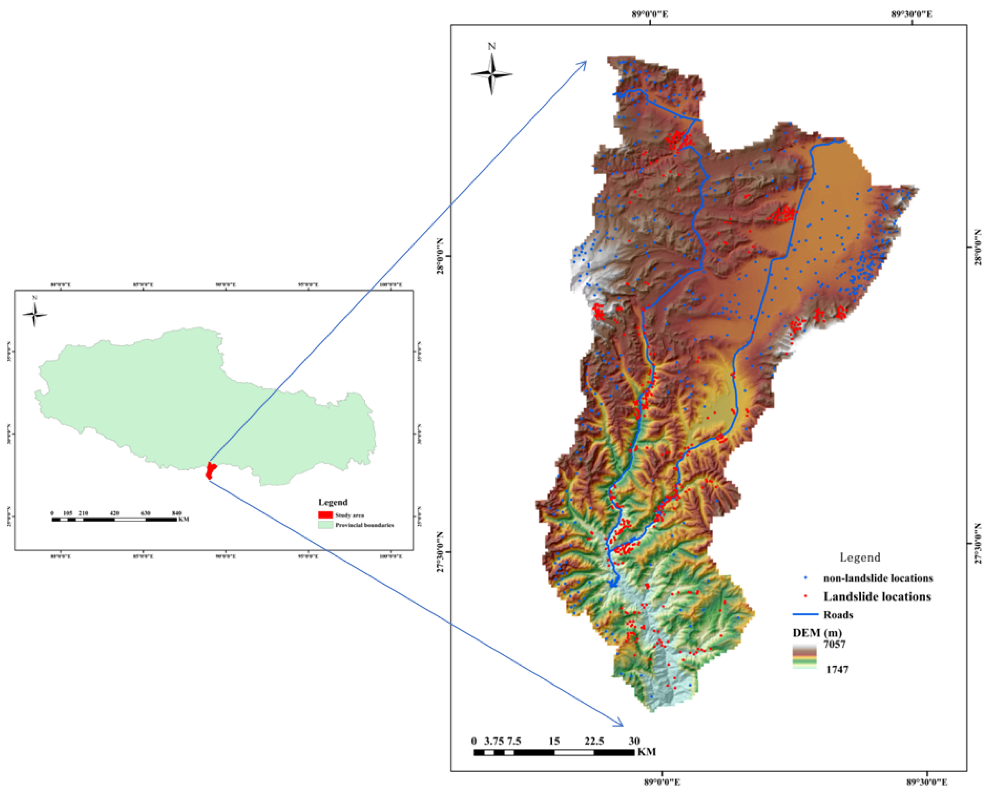
Yadong County is under the jurisdiction of Shigatse City, Tibet Autonomous Region, at the southern foot of the middle section of the Himalayas (
Figure 1). Over 120,000 people live in the study area, which extends over some 4240 km
2. It belongs to the high mountain landform of the Himalayas with an average elevation of 3500m (ranging from 1747~7057 m). The study area is divided into two parts, north and south, based on the line from Pali Town to Kangbu Town due to the great difference in altitude and two completely different climates are formed [
5]. The northern region is 4300m above sea level, with a cold and dry climate and an average annual rainfall of about 410mm. The altitude in the south has dropped significantly, with an average altitude of 2800 meters, a humid climate, and an annual precipitation of 873 mm. This study area has mainly shale, limestone, and dolomite. In the southern area of the study area, faults and folds dominate the geology. There is a degree of VIII on the modified Mercalli index indicating a high seismic intensity. The density of geological disasters in the southern area is relatively high, mainly collapses and landslides, while the northern area is dominated by debris flows.
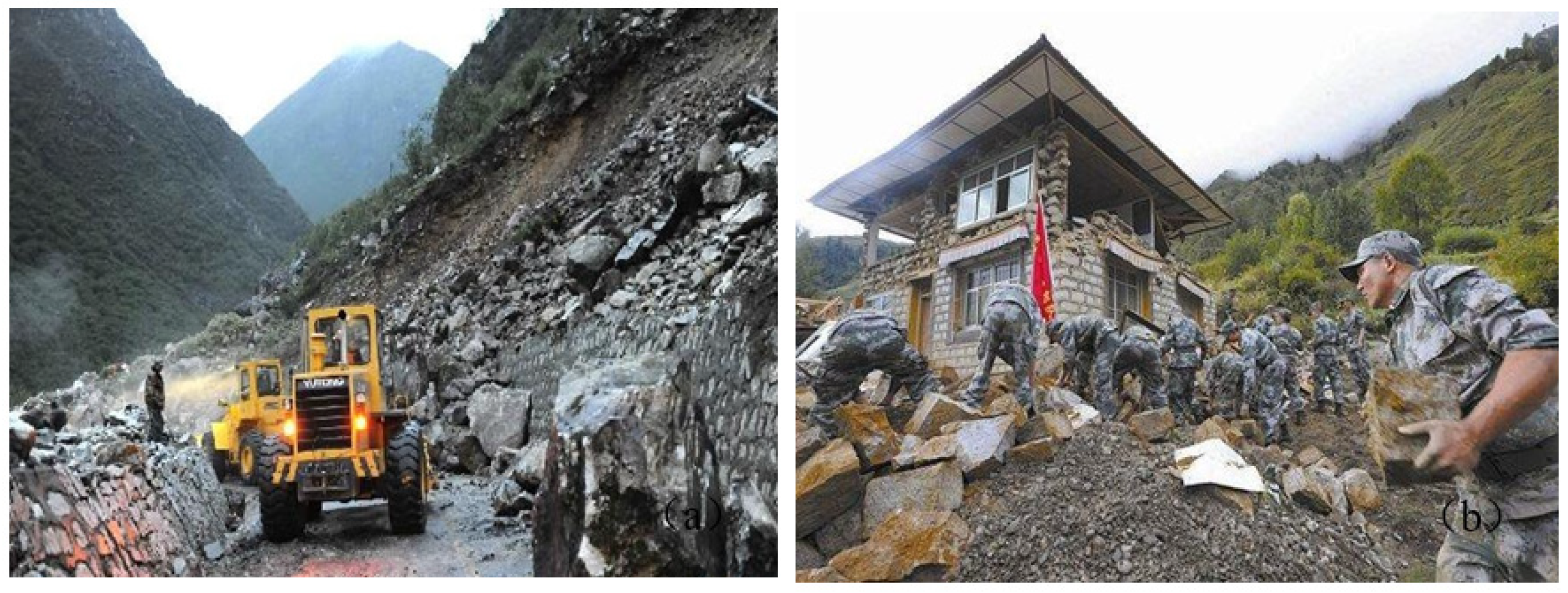
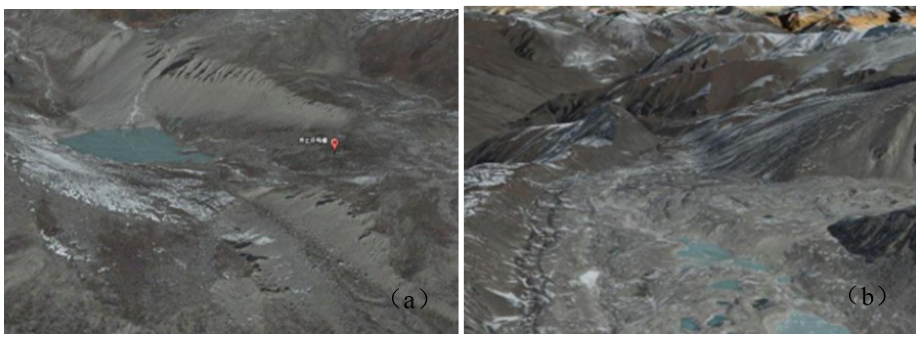
On September 18, 2011, a magnitude 6.8 earthquake occurred in Sikkim, India. The study area was affected by the earthquake which induced a series of secondary geological disasters, causing great harm to local residents and roads (
Figure 2 and
Figure 3). Therefore, it is of great significance to compile an accurate landslide susceptibility map for the study area.
2.2. Data preparation
2.2.1. Landslide inventory
Typically, data-driven methods for LSM assume that landslides have a greater chance of recurring under the same conditions as they did before [
25]. Therefore, a comprehensive and exact landslide inventory that shows the locations and numbers of landslides is essential [
7]. It is therefore essential to develop a complete and accurate landslide inventory (
Figure 4) that shows the locations and quantities of landslides. This data can be obtained by taking aerial photographs, reading literature, and conducting extensive fieldwork. Landslides are bounded by polygons containing the entire perimeter, and 496 polygons representing the landslide perimeter were identified. Using a 1:1 sampling strategy [
26], the model was trained and validated with 992 samples, including 496 landslides with a sign of “1” and 496 non-landslides with a sign of “0”. Non-landslide samples were randomly selected from non-landslide dense areas.
2.2.2. Conditioning factors
A total of 11 conditions factors were selected based on the study region's characteristics, the data's availability, reliability, and practicality, including elevation, slope, maximum elevation difference, plan curvature, profile curvature, topographic wetness index, distance to faults, distance to roads, distance to streams, annual rainfall and NDVI [
27].
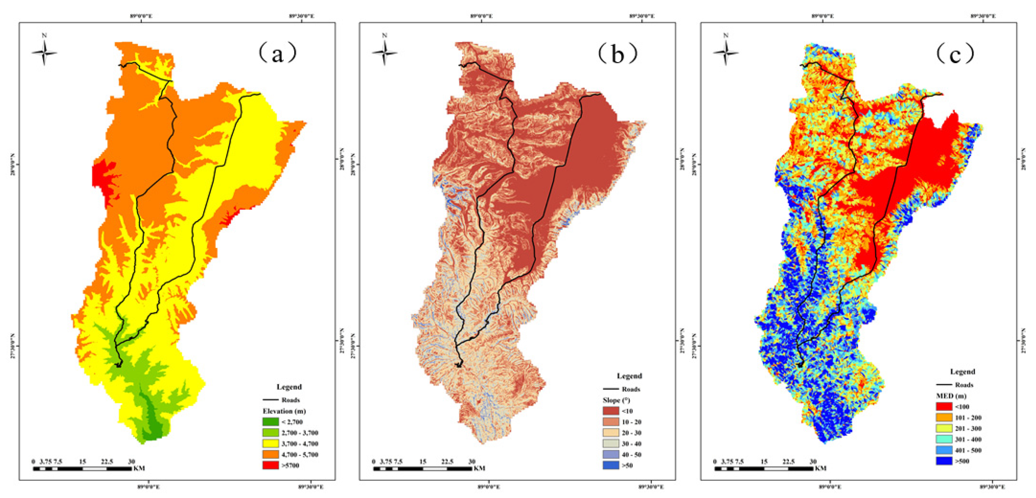
Elevation which was divided into five sub-classes by 1000 m intervals, has an influence on both rainfall and vegetation [
28,
29] (
Figure 4a). Slope, which controls shear strength at potential slide surfaces as well as subsurface flow [
30], was reclassified into six classes by 10° intervals (
Figure 4b). It was calculated in ArcGIS 10.2 that the maximum elevation difference reflects potential kinetic energy of slope units. By 100 m intervals, the thematic map was reclassified into six classes (
Figure 4c). Erosion and deposition can be determined from slope curvature since it is essential to the geometry of slopes [
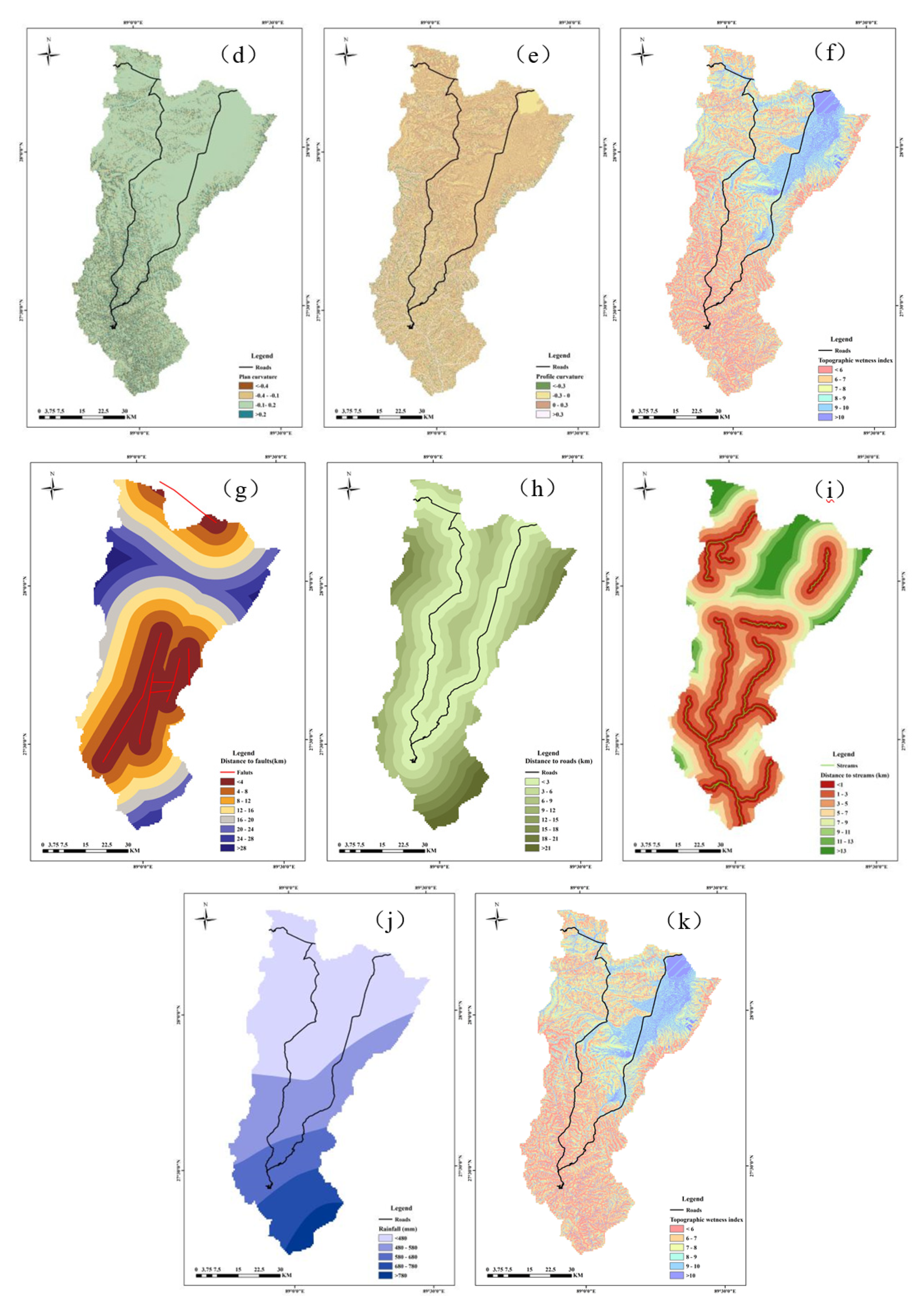
31]. Six classes were established for profile and plan curvatures (
Figure 4d and 4e). The TWI represents basic terrain, which was divided into six categories (
Figure 4f). With the spatial resolution of 30 meters, six topographic factors were extracted from the digital elevation model (DEM).
Bulk-rock strength could be reduced as a result of faults acting as potential weak planes in slopes and distance to fault was constructed with six classes by 2000m intervals (
Figure 4g). In a similar manner, distances to the road and river were divided into six categories with an interval of 2000 meters (
Figure 4h,i).
An existing 1:50,000 geological map was used to extract fault information, and Landsat 8 LOI images were used to determine road and river network information. Using the Euclidean Distance ArcGIS Tool, the distances from each raster unit of the area to the nearest fault, road, stream, and highway were calculated.
The unique trigger factor considered in the study was rainfall, and it has been applied numerous times. Based on the data from 14 precipitation stations near the study area, an ordinary kriging interpolation was used to generate the thematic map in ArcGIS. The thematic map was reclassified into 4 classes (
Figure 4j).
The consolidation of vegetation roots can stabilize soil, which alleviates the effect of rainfall on the stability of the slope [
34]. The Vegetation normalization index(NDVI) was applied to evaluate the vegetation and it is calculated by:
Where RED is the reflection value of the red wavelength and NIR is the near-infrared wavelength.
NDVI ranges from -1~1 with a positive value indicating coverage and the greater the value, the greater the coverage. The thematic map was reclassified into 6 classes (
Figure 4k)
2.2.3. Mapping units
LSM commonly uses grid cells, slope units, and unique-condition units as mapping units. The choice of mapping unit is controversial, however, grid cells are the most common [
35,
36]. Landslides can be represented better by a slope unit, which represents their source, transport, and accumulation areas. Thus, the study area is divided into 25483 slope units with the hydrologic analysis tool in ArcGIS and necessary artificial corrections are accompanied according to remote sensing images.
3. Methods
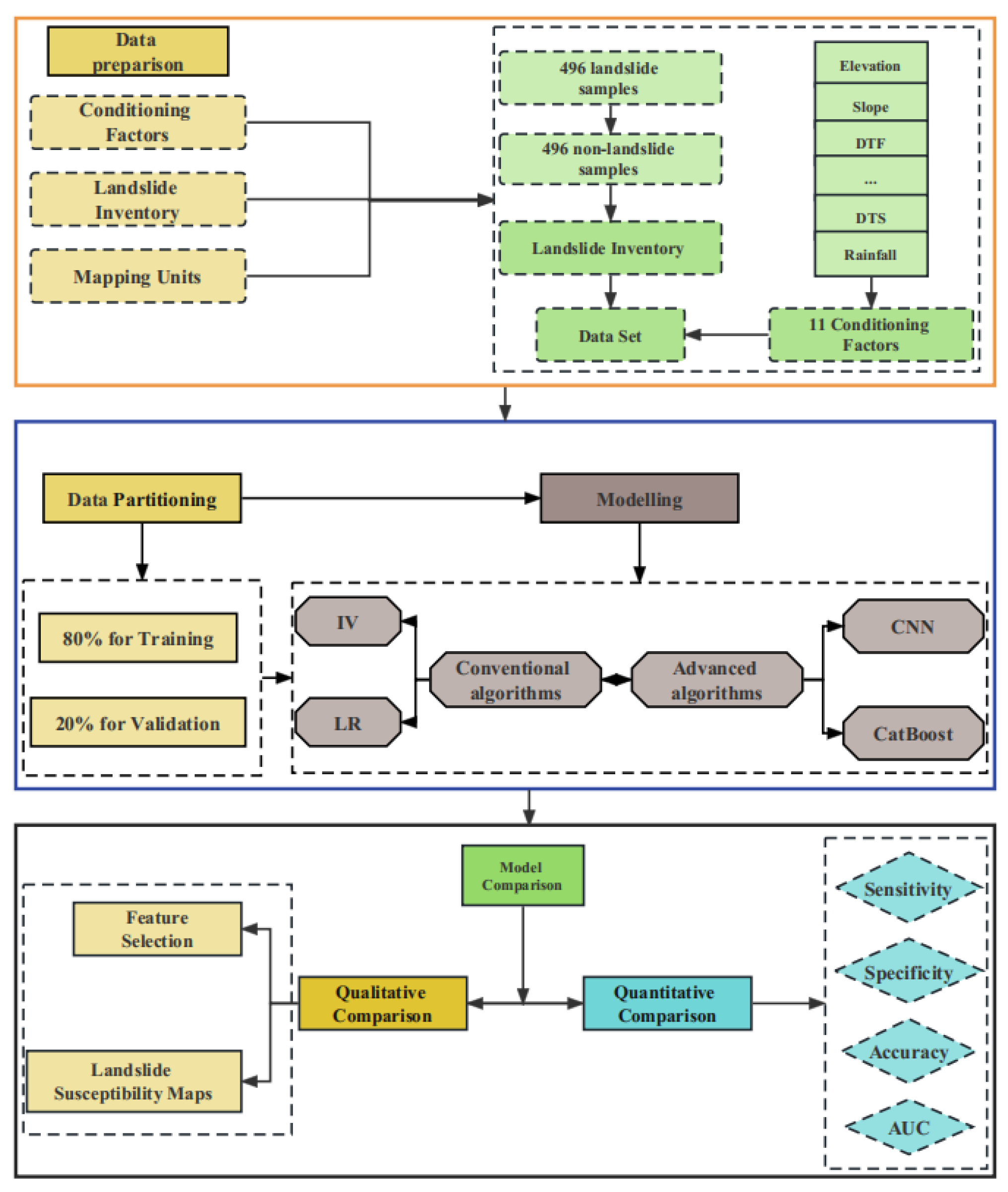
The main aims of the study are to explore and compare the effect of conventional and advanced modeling algorithms on Landslide susceptibility prediction. The methodology followed in this study mainly contains five steps (
Figure 5). Firstly, data sets including landslide samples, conditioning factors, and mapping units are prepared for modeling. The second is to divide the data set into training and validation parts. After that, four representative algorithms as IV, LR, CatBoost, and CNN are applied to LSM. Finally, the performance of LR, CatBoost, and CNN models are analyzed and compared based on some key measures.
3.1. IV
By using the frequency or density of landslides, the IV method reflects the magnitude of the hazards associated with different influencing factors and their sub-intervals. IV was first proposed by Yin and Yan (1988) and later modified by Van Westen (1993) [
38]. Equation 1 shows the method for the calculation of the information values:
Where i=1, 2, 3, …, n; j = 1, 2, 3, …, m; si-j represents the area of the landslide of the i-th conditioning factor in j-th interval; ni-j represents the area of the i-th conditioning factor in j-th interval; S represents the total area of the landslide; N represents the total area.
Depending on the IV method, the value might be positive or negative. When IV values are positive, they indicate that the factor is conducive to the occurrence of landslides in a particular interval: a higher IV indicates a higher likelihood of landslides, and vice versa.
The total information value I can be determined by:
Finally, the information value calculated by each unit is processed by linear normalization.
3.2. LR
The LR model is used for statistical analysis of binary dependent variables (the dependent variable y has two values: 0 and 1) [
39]. The LR model is advantageous since the data distribution can either be nominal or continuous [
40]. It is computed using the following equation:
where p represents the occurrence probability of an event (such as a landslide) on the s-curve in the range of 0 to 1; y represents a linear combination function and is calculated by using Eq.5.
Where b0 is the constant value or intercept of the equation, and b1, b2, ..., bn are the regression coefficients of the explanatory variables x1, x2, ..., xn.
In the current study, the LR model was performed in SPSS software, the and forward stepwise method was adopted to screen valuation indexes. The conditioning factors were calculated as independent variables, whereas dependent variables represent the occurrence of landslides. During the last step of the analysis, all variables were significant at less than 0.05, so no additional variables were included.
3.3. CatBoost
CatBoost is an improved implementation based on Gradient Boosted Decision Tree (GBDT) framework, with fewer parameters. It is an open-source machine-learning library of Yandex and a member of Boosting family. The gradient deviation and prediction offset can be effectively solved by CatBoost algorithm, so as to reduce the occurrence of over-fitting and improve the accuracy and generalization ability of the algorithm [
41]. Detailed information about CatBoost can be referred to another literature [
42].
3.4. CNN
CNN provides an end-to-end learning model that can select model parameters through traditional gradient descent methods. The trained CNN can learn image features and complete the extraction and classification of image features [
43]. A CNN consists of the network structures as convolutional layer, down-sampling layer, and fully connected layer, each of which contains a number of independent neurons [
44]. Its notable feature is that the weight sharing and local connection of the convolution kernel in the hidden layer can greatly reduce the number of weights, thereby reducing the complexity of the convolutional network model.
The unique convolutional layer and pooling layer structure of CNN can be combined arbitrarily to obtain an infinite variety of network models. This study applied the AlexNet model to LSM [
45]. Before modeling, conditioning factors are requested to be superimposed to obtain a multi-band two-dimensional image as the input raw data in LSM. Since LSM belongs to a two-classification problem of landslide disasters, two neurons are placed in the output layer classifier to represent landslide and non-landslide. All parameters have been optimized through trial and error approach. The number of training cycles is 10, the initial learning rate is 0.01, the loss function uses standard cross-entropy, the optimizer is Adam, and the activation function is Relu.
The machine learning and deep learning-based algorithms are implemented in Python3.7 based on the Package of Numpy, Scikit-Learn, and Tensorflow. The statistics-based algorithms are implemented in SPSS.
3.5. Models evaluation
A predictive model will not be convincing without scientific validation, so existing data will need to be split into training and validation sets. There were 80% of the data sets randomly chosen for training and 20% for validation in LSM.
Four evaluation measures as accuracy, sensitivity, specificity, and AUC were combined to analyze the performance of the models. Accuracy, sensitivity ,and specificity are calculated from the Confusion Matrix, which is an N × N matrix (
Table 2). The TP represents the number of landslides that have been correctly predicted as unstable and TN represents the number of non-landslides that have been correctly predicted as stable. While FP represents the number of non-landslides that have been predicted incorrectly as unstable and FN represents the number of landslide units that have been predicted incorrectly as stable.
Table 1.
Landslide conditioning factors in this study.
Table 1.
Landslide conditioning factors in this study.
| Conditioning Factors |
Zone |
Ni/N |
Si/S |
IV |
| Elevation (m) |
<2700 |
1.21% |
1.09% |
0.100 |
| 2700~3700 |
21.98% |
8.26% |
0.978 |
| 3700~4700 |
43.80% |
49.88% |
-0.131 |
| 4700~5700 |
28.63% |
39.29% |
-0.317 |
| >5700 |
4.44% |
1.48% |
1.098 |
| Slope (°) |
<10 |
11.90% |
35.95% |
-1.106 |
| 10~20 |
25.60% |
29.88% |
-0.154 |
| 20~30 |
38.31% |
25.67% |
0.400 |
| 30~40 |
22.18% |
8.13% |
1.003 |
| >40 |
2.02% |
0.36% |
1.709 |
| MED (m) |
<100 |
7.46% |
36.41% |
-1.585 |
| 100~200 |
13.91% |
21.80% |
-0.449 |
| 200~300 |
11.90% |
15.82% |
-0.285 |
| 300~400 |
20.56% |
10.76% |
0.648 |
| >400 |
46.17% |
15.21% |
1.110 |
| Plan curvature |
<-0.4 |
0.20% |
0.12% |
0.538 |
| -0.4~-0.1 |
4.44% |
4.89% |
-0.097 |
| -0.1~0.2 |
92.74% |
93.11% |
-0.004 |
| >0.2 |
2.62% |
1.89% |
0.328 |
| Profile curvature |
<-0.3 |
0.20% |
0.59% |
-1.078 |
| -0.3~0 |
31.20% |
36.57% |
-0.157 |
| 0~0.3 |
67.54% |
62.50% |
0.077 |
| >0.3 |
1.01% |
0.33% |
1.106 |
| TWI |
<6 |
7.26% |
5.85% |
0.215 |
| 6~7 |
46.57% |
32.13% |
0.371 |
| 7~8 |
33.27% |
27.54% |
0.189 |
| 8~9 |
8.87% |
14.48% |
-0.490 |
| 9~10 |
2.42% |
9.11% |
-1.326 |
| >10 |
1.61% |
10.89% |
-1.910 |
| Distance to faults (km) |
<4 |
31.05% |
20.27% |
0.426 |
| 4~8 |
16.33% |
14.71% |
0.105 |
| 8~12 |
7.46% |
14.57% |
-0.670 |
| 12~16 |
22.18% |
16.00% |
0.327 |
| 16~20 |
14.31% |
14.99% |
-0.046 |
| 20~24 |
8.67% |
12.22% |
-0.343 |
| 24~28 |
0.60% |
6.10% |
-2.311 |
| >28 |
0.20% |
1.14% |
-1.734 |
| Distance to streams (km) |
<1 |
47.58% |
14.51% |
1.187 |
| 1~3 |
19.35% |
25.62% |
-0.280 |
| 3~5 |
7.06% |
19.97% |
-1.040 |
| 5~7 |
6.65% |
14.66% |
-0.790 |
| 7~9 |
9.07% |
11.07% |
-0.199 |
| 9~11 |
5.44% |
7.00% |
-0.252 |
| 11~13 |
3.63% |
4.38% |
-0.189 |
| >13 |
1.61% |
2.78% |
-0.544 |
| Distance to roads (km) |
<3 |
57.66% |
32.20% |
0.583 |
| 3~6 |
11.69% |
25.23% |
-0.769 |
| 6~9 |
14.11% |
18.23% |
-0.256 |
| 9~12 |
6.20% |
9.08% |
-0.374 |
| 12~15 |
5.44% |
6.37% |
-0.158 |
| 15~18 |
1.41% |
4.46% |
-1.151 |
| 18~21 |
2.62% |
2.07% |
0.237 |
| >21 |
0.81% |
2.35% |
-1.070 |
| Average annual precipitation (mm) |
<480 |
32.26% |
50.99% |
-0.458 |
| 480~580 |
29.44% |
24.55% |
0.182 |
| 580~680 |
24.60% |
11.55% |
0.756 |
| 680~780 |
3.02% |
9.38% |
-1.132 |
| >780 |
10.69% |
3.53% |
1.107 |
| NDVI |
<0.15 |
16.53% |
12.68% |
0.265 |
| 0.15~0.3 |
25.20% |
36.62% |
-0.374 |
| 0.3~0.45 |
15.12% |
19.74% |
-0.266 |
| 0.45~0.6 |
15.93% |
17.94% |
-0.119 |
| 0.6~0.75 |
22.18% |
9.93% |
0.804 |
| >0.75 |
5.04% |
3.09% |
0.490 |
An additional indicator of model validity is the area under the receiver operating characteristic curve (AUROC). The value of AUROC ranges from 0.5~1, the larger the value, the better the generalization ability of the model and prediction performance.
4. Results
4.1. Performance and comparison of conventional and advanced algorithms
Before modeling, the data were normalized with Z-scores to eliminate the effects of different dimensions. Additionally, a correlation analysis was conducted to test the collinearity among the independent variables using the variance inflation factor (VIF) [
44]. There is severe col-linearity between the selected variables if the VIF value exceeds 10.
Table 2 showed the VIF values of the chosen independent variables and the factor Elevation has the highest VIF value (5.711). The result indicates that no severe collinearity problems exist among the chosen variables and thus, 11 conditioning factors were applied to the modeling.
The performance of the three models using the confusion matrix is shown in Table 5. The CNN model achieved the highest value of sensitivity (84.21%), followed by the CatBoost model (sensitivity=82.96%) and the LR model (sensitivity =81.45%). As for specificity, the CNN model performed best with 93.52%, followed by the CatBoost model with 86.63 % and the LR model with 84.79%. The CNN model also ranked the first for specificity with a value of 93.52%, followed by CatBoost (86.63%) and LR (84.79%). CNN model had the best accuracy and ROC values of 88.88% and 0.944, while the LR model had the worst values of 83.13% and 0.897. As well, CatBoost performed well, scoring 86.63% and 0.930 respectively.
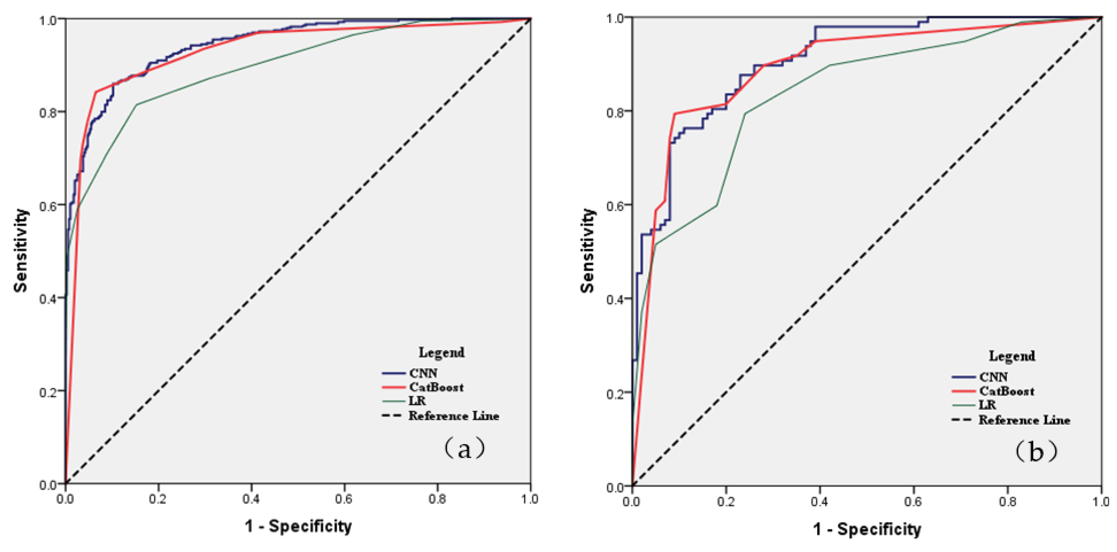
The verification data set is more useful and important for evaluating the ability of these models to generalize. In
Figure 6, we found that the CNN model had the highest sensitivity, specificity, accuracy, and AUC values, namely 79.38%, 91.00%, 85.28%, and 0.908. Additionally, CatBoost performed well with 76.28%, 85.00%, 80.71%, and 0.893, respectively. The LR model remained the worst with values of 79.38%, 76.00%, 77.66%, and 0.838 (Table 5).
Model performance declined in verification, particularly for the LR and CatBoost models (the accuracy value decreased by about 6%), which indicated that the models were overfitting and generalizability was suspicious. While the performance of the CNN model was stable as the value of AUC reached 0.908 and the accuracy value was close to the training data set.
4.2. Landslide susceptibility mapping results
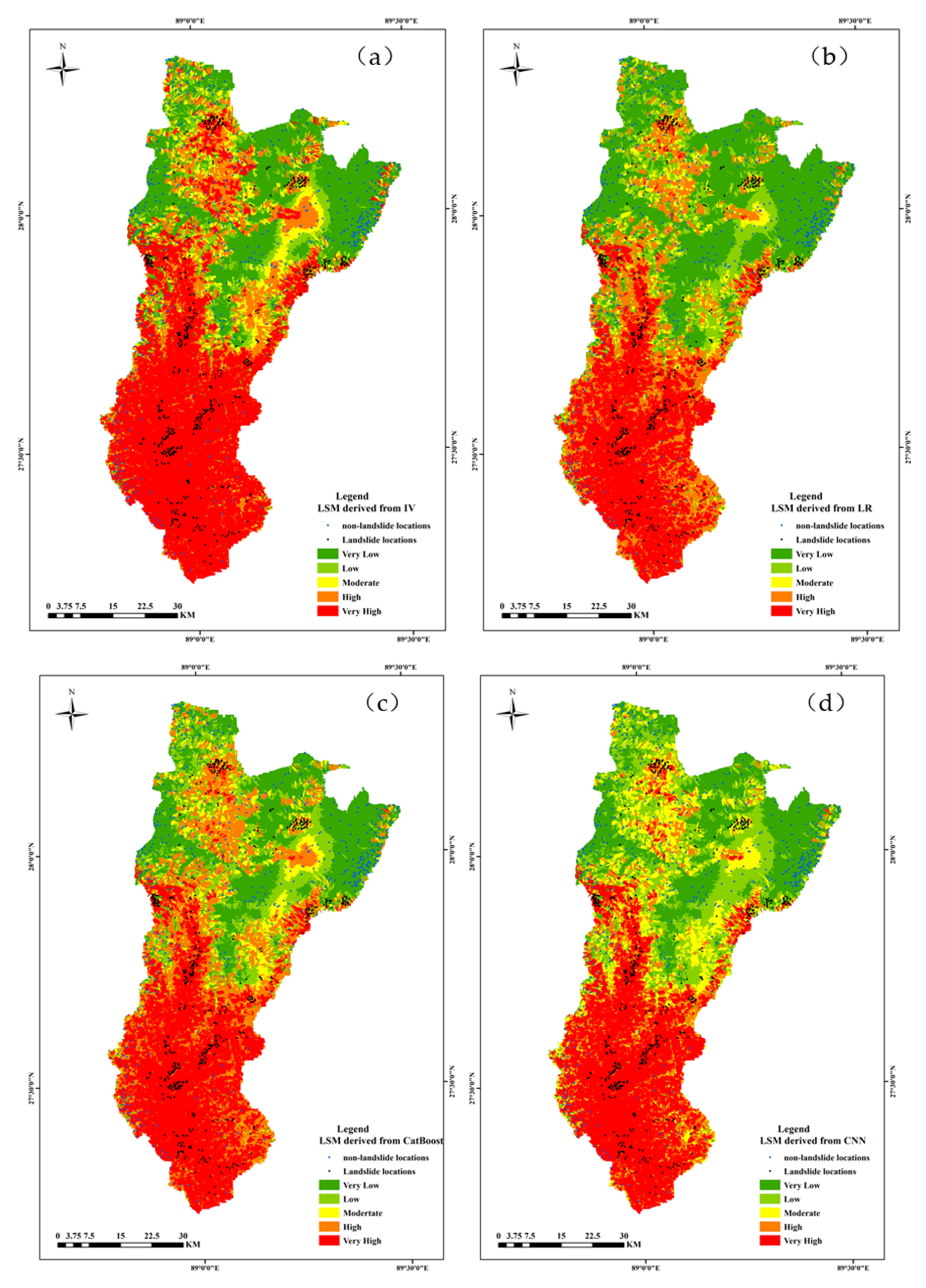
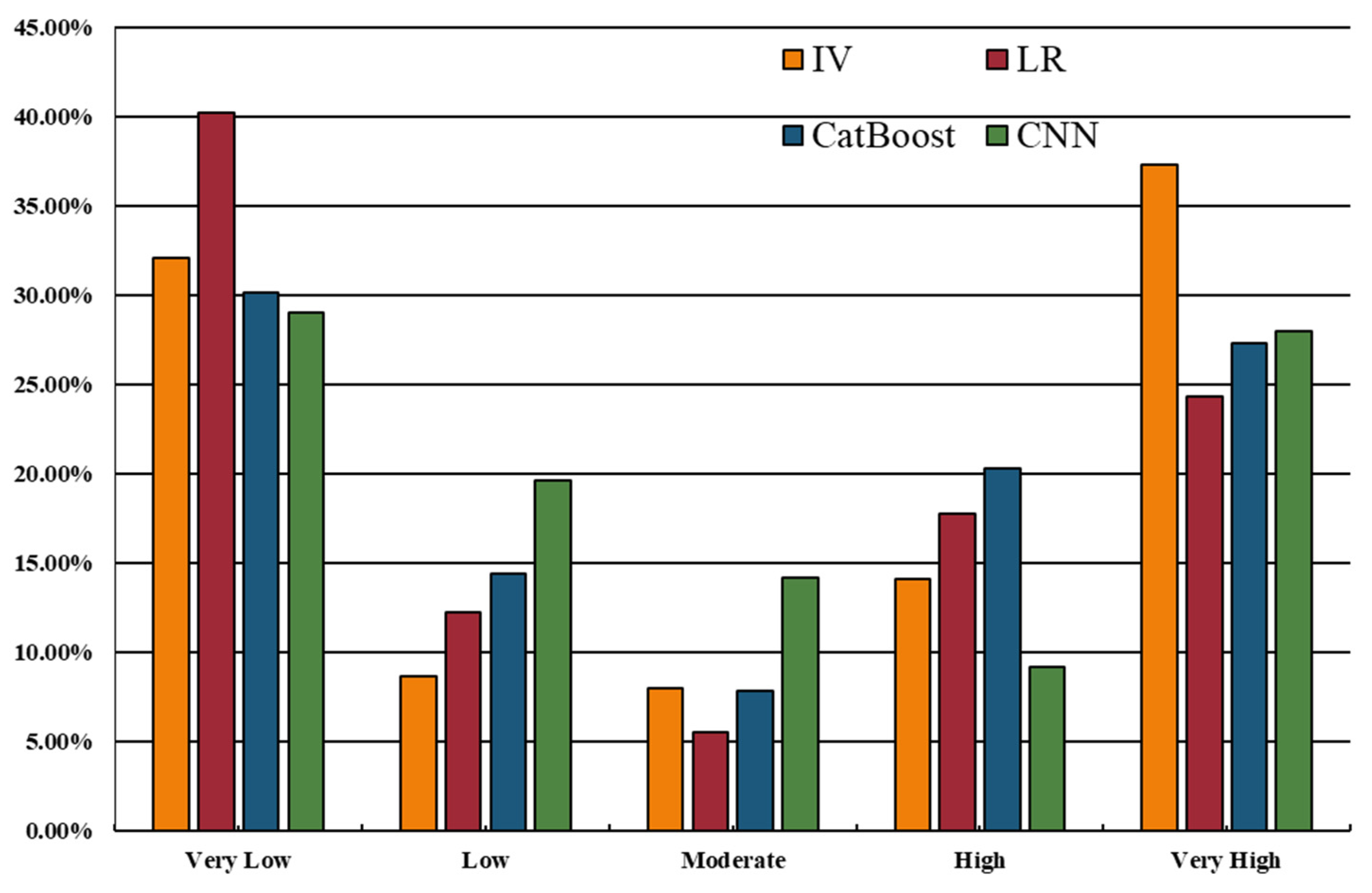
In case of LR model, LSI ranges from 0.11 to 0.96, and the corresponding area percentages were 40.17% (very low), 12.24% (low), 5.54% (moderate), 17.75% (high) and 24.30% (Very high), respectively. Similarly, five reclassified classes of the CatBoost model accounted for 30.16%, 23.81 %, 15.21 %, 26.82 %, and 14.94 % respectively of the entire area. LSM constructed by the CNN model was also divided into five classes: very low (<0.18), low (<0.42), moderate (<0.653), high (<0.82), and very high (>0.82), accounting for 28.99%,19.65%,14.21%,9.19% and 27.96% of the whole area. It is noticed that LR, CatBoost, and CNN models predicted the largest proportion of very low susceptibility while IV predicted the largest proportion of very high susceptibility.
A logical landslide susceptibility map should meet two rules: (1) the density of landslide samples should increase with the increase of susceptibility class and be mainly located in the highest susceptibility area; (2) the landslide susceptibility map should be spatially continuous and smooth and the very high-susceptibility class area should occupy a small proportion. Concomitant with these maps (
Figure 7), the landslide samples (dark spots) were mainly located in the red areas, and the non-landslide samples (blue spots) were in the green areas. The high or very high susceptibility areas were concentrated in the south of the areas, which was consistent with the distribution of landslides (
Figure 8). Thus, the maps predicted by these models were logical on the whole.
There are distinct differences among the landslide susceptibility maps derived from the models.
Table 2 showed that the IV increased as the susceptibility class increased for the model and the IVs were all negative for the very low, low, and moderate susceptibility class while positive for the very high susceptibility class. For high susceptibility, the IVs were positive for LR, CatBoost, and CNN models while negative for the IV model. On the other hand, the maps predicted by IV and LR models were spatially discontinuous while CatBoost and CNN models produced smoother patterns. Besides, the percentage of very high susceptibility class was similar for LR, CatBoost, and CNN models, while the IV model predicted the highest percentage reaching 37.27%.
In comparison to the other 3 models, the CNN model shows superior fitting and generalization capabilities in predicting landslide susceptibility. It has been found that very high landslide susceptibility areas are mainly associated with the Yarlung Zangbo River and its tributaries. A large part of the eroded slopes is scoured by the river network. The areas near streams are densely populated, and the occurrence of landslides can threaten lives.
4.3. Evaluation of conditioning factors
4.3.1. Application of conventional algorithms
Bivariate methods were used to establish relationships between the conditioning factors and the occurrence of the landslides, as shown in
Table 1. As for elevation, the percentages of landslide area for 3700~4700m and 4700~5700m were 43.80% and 28.63% respectively, which means that over 70% of landslide areas were distributed among the two classes but the IV value of these two classes were both negative. While the highest IV of elevation is 1.098 for the class of >5700. For Slope, the IV values increased as the slope increased, as well as the factor MED, which indicated that landslides are more likely to occur in steep areas. The IV of slope ranged from -1.106~1.709, in which the classes of >20 were all positive. In terms of TWI, the class of 6~7 had the highest IV of 0.371 and the IV were all negative at the class of >8.
For curvature, the highest IV of plan curvature was 0.538, located at the class of <-0.4, and 1.106 of Profile curvature at the class of >0.3. It was found that landslides were concentrated in convex terrain. On the other hand, landslides are highly concentrated near the faults, streams, and roads as the IV reached the maximum value at first class. It indicated that the development of faults, streams, and human engineering activities was conducive to the occurrence of landslides.
As for rainfall, the highest probability of landslides occurring appeared in the class of >780mm (IV reached 1.107). While the IV did not increase with increasing rainfall and it indicated that landslide occurring is complex. In case of NDVI, the class of 0.6~0.75 has the highest IV of 0.804. The IV changed erratically for NDVI although high vegetation cover helped enhance the stability of the landslide.
As for the LR model, the final regression equation is as followed:
It can be found that MED, rainfall and DTR were essential to landslide occurring as the coefficients were relatively large. While profile curvature and DTS were considered as secondary factors. The coefficient of DTR was negative, which indicated a negative effect on landslide occurring.
Conventional algorithms such as IV and LR methods were used to establish the relationships between the conditioning factors and the occurrence of the landslides in this study. In summary, the conditioning factors have an effect on landslides occurring and the impact of different factors on landslides varies in different intervals.
4.1.2. Application of advanced algorithms
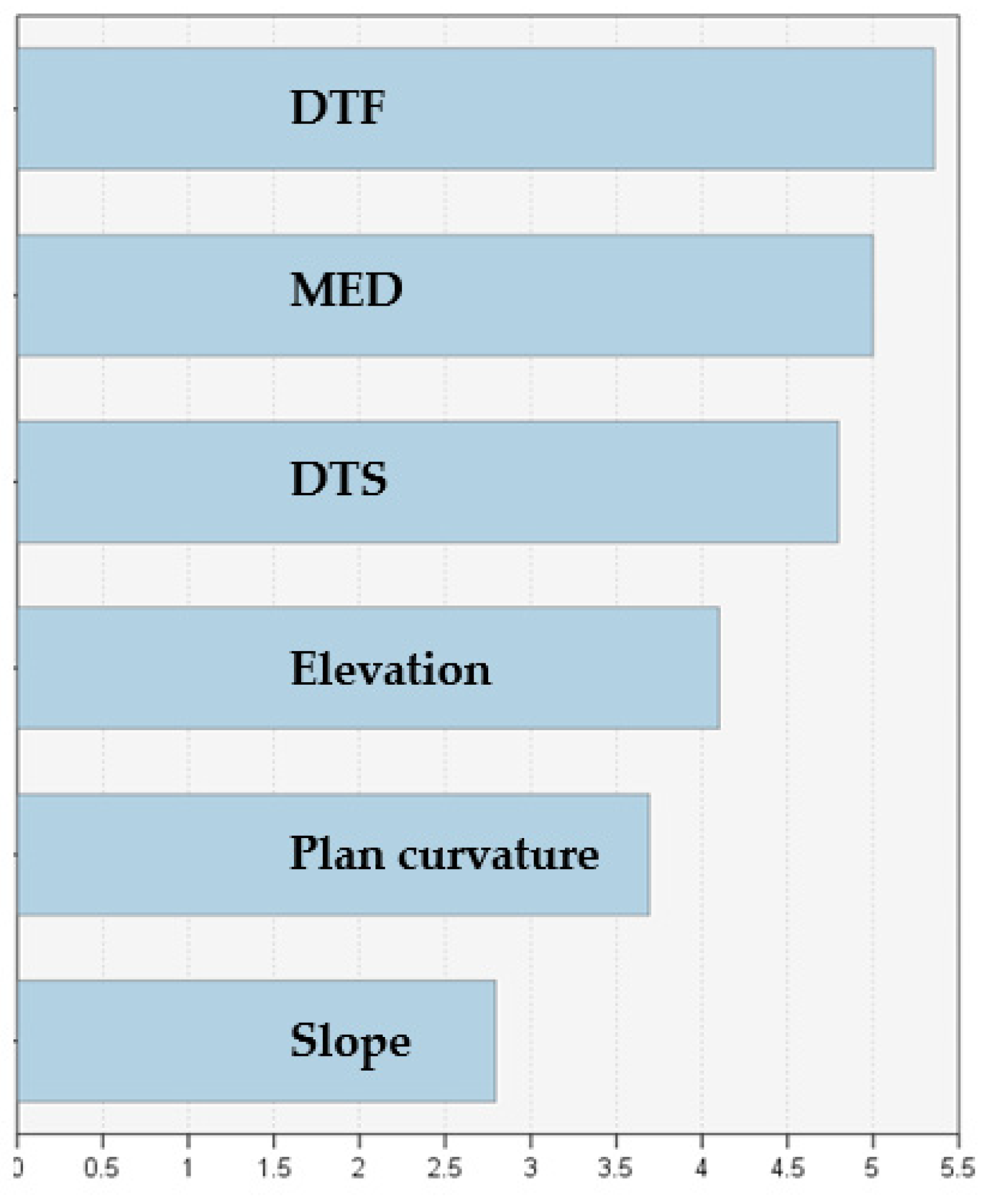
Actually, conditioning factors have different influences on the occurrence of landslides while the bivariate methods fail to recognize the difference. Gini importance (GI) is defined as the total reduction in average nodal impurities across all trees. GI was also applied to analyze the relative importance of different factors, exploring the factor’s contribution to landslide occurring.
The bigger the GI express greater the importance of factors of landslides occurring [
44].
Table 3 showed the rank of the conditioning factors of this study. The result showed that DTF was the most important factor responsible for landslides as the GI reached 5.36. Besides, the factor MED, DTS, elevation, plan curvature, and slope were also pivotal since the GI were all greater than zero. While the other factors as TWI, rainfall, profile curvature, NDVI ,and DTR showed little contribution to landslides in the study area (
Figure 9).
Table 3.
Multicollinearity diagnosis indexes for variables.
Table 3.
Multicollinearity diagnosis indexes for variables.
| Variables |
VIF |
| Elevation |
5.117 |
| Slope |
3.426 |
| MED |
5.726 |
| Plan curvature |
1.499 |
| Profile curvature |
1.291 |
| TWI |
6.071 |
| Distance to fault |
2.641 |
| Distance to stream |
4.492 |
| Distance to road |
4.302 |
| Average annual precipitation |
1.763 |
| NDVI |
2.697 |
Table 4.
Models’ performance using related indices.
Table 4.
Models’ performance using related indices.
| |
Training |
Validation |
| Parameter |
LR |
CatBoots |
CNN |
LR |
CatBoots |
CNN |
|
Sensitivity(%)
|
81.45 |
82.96 |
84.21 |
79.38 |
76.28 |
79.38 |
|
Specificity(%)
|
84.79 |
90.27 |
93.52 |
76.00 |
85.00 |
91.00 |
|
Accuracy(%)
|
83.13 |
86.63 |
88.88 |
77.66 |
80.71 |
85.28 |
| AUC |
0.897 |
0.930 |
0.944 |
0.838 |
0.893 |
0.908 |
Table 5.
The IV of different landslide susceptibility levels.
Table 5.
The IV of different landslide susceptibility levels.
| Model |
Class |
Percentage of area (%) |
Percentage of landslide area (%) |
IV |
| IV |
Very low |
32.05% |
8.06% |
-1.74 |
|
| Low |
8.64% |
7.66% |
-1.19 |
|
| Moderate |
7.96% |
5.04% |
-0.50 |
|
| High |
14.08% |
20.36% |
-0.14 |
|
| Very high |
37.27% |
58.87% |
0.70 |
|
| LR |
Very low |
40.17% |
5.24% |
-1.60 |
|
| Low |
12.24% |
4.44% |
-0.47 |
|
| Moderate |
5.54% |
6.05% |
-0.10 |
|
| High |
17.75% |
21.17% |
0.14 |
|
| Very high |
24.30% |
63.10% |
0.88 |
|
| CatBoost |
Very low |
30.16% |
5.24% |
-1.74 |
|
| Low |
14.42% |
4.44% |
-1.18 |
|
| Moderate |
7.82% |
6.05% |
-0.25 |
|
| High |
20.28% |
21.17% |
0.04 |
|
| Very high |
27.31% |
63.10% |
0.84 |
|
| CNN |
Very low |
28.99% |
4.44% |
-1.88 |
|
| Low |
19.65% |
8.67% |
-0.82 |
|
| Moderate |
14.21% |
12.30% |
-0.14 |
|
| High |
9.19% |
11.09% |
0.19 |
|
| Very high |
27.96% |
63.51% |
0.69 |
|
Table 5.
Conditioning factors assigned by the Gini index.
Table 5.
Conditioning factors assigned by the Gini index.
| Method |
DTF |
MED |
DTS |
Elevation |
Plan curvature |
Slope |
| Gini index |
5.36 |
5.00 |
4.80 |
4.10 |
3.69 |
2.80 |
Figure 9.
Parametric importance graphics designed by Gini index.
Figure 9.
Parametric importance graphics designed by Gini index.
4. Discussion
With the progress of related technologies and the maturity of theory, various approaches have been developed and applied to LSM to improve prediction accuracy and reliability [
47,
48,
49]. Recently, deep learning is becoming popular and beginning to be used for LSM. In this study, CNN was applied to LSM, and its performance was compared to the conventional statistical methods and machine learning approaches.
Different algorithms have different emphases and generally, their performance varies with different study areas [
50,
51]. However, advanced algorithms usually perform better in terms of accuracy compared to conventional statistical methods [
52,
53]. The result of our study also found that CNN and CatBoost performed better in terms of accuracy and CNN did the best in generalization. There was a certain gap between the three models. The improvement benefits from the characteristics of the algorithms themselves for decreasing the bias, discrepancy, and over-fitting problems. It is easy to implement and acceptable in conventional statistical methods to establish a mathematical equation for investigating the relationship between factors related to landslides and landslides occurring. In machine learning methods, optimization is stressed, so the multiple parameters involved need to be tuned before application, which is challenging for non-experts [
54,
55]. Deep learning algorithms use a more complex modeling architecture consisting of convolutional, activation, pooling, and fully connected layers, taking images as input parameters. Feature selection and information filtration are done in the pooling layer, which is a robust step in CNN. Importantly, the dimensionality reduction is done without changing the depth of the maps. Thus, deep learning algorithms have the ability to process data efficiently, feature extraction of high-dimensional data and keep high prediction accuracy.
The accuracy of LSM should not be the only priority. Identifying the major conditions that lead to landslides is also critical, which assists in furthering the process. Identifying subjective weights and objective weights allows for separating their contributions. Analytic hierarchy processes (AHP) and factor analyses (FA) are commonly used methods [
58,
59]. Landslide and their underlying conditioning factors can be directly correlated using LR models [
60,
61]. The relative importance of factors can be determined by the magnitude, plus or minus of the coefficients. In addition, bivariate methods are capable of distinguishing factors with different susceptibilities to landslides across interval ranges. Accordingly, LR and IV are recommended to be combined to analyze the factor’s contribution to landslide occurring. GI describes the contribution of the conditioning factors by calculating the total decrease and the final coefficients reflect the relative importance of different factors. Some studies have applied GI for feature selection, which helps to decrease redundant information [
62,
63].
As for bivariate methods like IV, FR, and CF, the performance is mainly up to whether the division of the conditioning factors interval is reasonable. However, there is no consensus on the size or number of intervals although some methods such as natural breaks and equal intervals have been applied. Besides, the total IV is a linear addition of the IV of all conditioning factors, which further amplifies the uncertainty of the final result. Thus, the susceptibility analysis of conditioning factors on different intervals by bivariate methods may unreliable and the landslide susceptibility maps are also difficult to be verified quantitatively. In terms of LR, the establishment of the equation derives from the distribution characteristics of data and is sensitive to linear correlation. Thus, the performance is up to data partition and will fluctuate during validation. The results of relative importance for conditioning factors may be confused or even contrary to our experience on landslides. Machine learning or deep learning emphasis on iterative operations and repeated verification and requires a large amount of data. Landslide samples are limited in a restricted area and difficult to collect. The performance will also decline as the data decrease.
6. Conclusions
In the current study, IV, LR were selected as representatives of the conventional algorithms, CatBoost and CNN as the advanced algorithms, for LSM in Yadong county, and their performance was compared. The following conclusions can be drawn:
1. There was a certain gap between the models. Compared to conventional algorithms, advanced algorithms performed better in terms of prediction accuracy and CNN performed the best in generalization, thus regarded as the best model in this study.
2. The landslide susceptibility map predicted by CNN was more reasonable and the very high susceptibility areas were mainly distributed along the Yarlung Zangbo River.
3. As for feature selection, IV and LR did a more detailed analysis of conditioning factors but the results were uncertain. The result analyzed by GI may be more reliable but fluctuates with the amount of data.
4. The conventional algorithms are inferior to the advanced algorithms in accuracy and feature selection but conventional algorithms have better resolvability and operability.
However, there are also some limitations of the present study:
There are possibilities for the combination of conventional and advanced algorithms and further exploration is needed to improve prediction accuracy obviously.
Models need to be validated more reliably.
Author Contributions
Z.L., writing—original draft, methodology and software; W.P., W.L., and Z.H., review and validation; M.L. and C.L., reviewing and editing. H.J., is responsible for the review and validation. All authors have read and agreed to the published version of the manuscript.
Funding
The completion of this work was supported by Guangzhou Collaborative Innovation Center of Natural Resources Planning and Marine Technology (No. 2023B04J0301), Key-Area Research and Development Program of Guangdong Province (NO.2020B0101130009), Guangdong Enterprise Key Laboratory for Urban Sensing, Monitoring and Early Warning (No.2020B121202019), The Science and Technology Foundation of Guangzhou Urban Planning & Design Survey Research Institute (Grant No. RDI2220204128, RDI2220204031, RDI2220204037)and Postdoctoral Research Project of Guangzhou (20220402).
Conflicts of Interest
The authors declare no conflict of interest.
References
- Das, I., Sahoo, S., Van Westen, C., Stein, A., Hack, R., 2010. Landslide susceptibility assessment using logistic regression and its comparison with a rock mass classification system, along a road section in the northern Himalayas (India). Geomorphology 114, 627–637. [CrossRef]
- Achour Y, BoumezbeurA, Hadji R, Chouabbi A, Cavaleiro V, Bendaoud EA (2017) Landslide susceptibility mapping using analytic hierarchy process and information value methods along a highway road section in Constantine, Algeria. Arab J Geosci 10 (194). [CrossRef]
- Arabameri, A., Pradhan, B., Rezaei, K., Lee, S., Sohrabi, M. An ensemble model for landslide susceptibility mapping in a forested area. Geocarto International, 1-26, 2019. [CrossRef]
- Ni, H. Y., Zheng, W. M., Li, Z. L., Ba, R. J.: Recent catastrophic debris flows in Luding county, SW China: Geological hazards, rainfall analysis and dynamic characteristics, Nat. Hazards, 55,523–542, 2016. [CrossRef]
- Liqiang Tong, Wensheng Qi, Guoying An,Chunling Liu. Remote sensing survey of major geological disasters in the Himalayas[J]. Journal of engineering geology, 2019, 27(03):496.
- Rai PK, Mohan K, Kumar VK (2014) Landslide hazard and its mapping using remote sensing and GIS. J Sci Res BHU 58 ISSN 0447-9483.
- Liang Zhu, Wang Changming, Han Songling, Kaleem Ullah Jan Khan, and Liu Yiao. Classification and susceptibility assessment of debris flow based on a semi-quantitative method combination of the fuzzy C-means algorithm, factor analysis and efficacy coefficient. Nat. Hazards Earth Syst. Sci., 20, 1287–1304, 2020a. [CrossRef]
- Corominas J, van Westen C, Frattini P, Cascini L, Malet J-P, Fotopoulou S, Catani F, Van Den Eeckhaut M, Mavrouli O, Agliardi F, Pitilakis K, Winter MG, Pastor M, Ferlisi S, Tofani V, Hervás J, Smith JT (2014) Recommendations for the quantitative analysis of landslide risk. Bull Eng Geol Environ 73:209–263. [CrossRef]
- Reichenbach,P.,Rossi,M.,Malamud,B.D.,et al.,2018.A Review of Statistically-Based Landslide Susceptibility Models. Earth-Science Reviews, 180(5): 60-91. [CrossRef]
- Shortliffe E H, Buchanan B G. A model of inexact reasoning in medicine [J]. Mathematical Biosciences, 1975, 23:351–379. [CrossRef]
- Korup O, Stolle A (2014) Landslide prediction from machine learning. Geol Today 30:26–33. [CrossRef]
- Chang K-T, Merghadi A, Yunus AP, Pham BT, Dou J. Evaluating scale effects of topographic variables in landslide susceptibility models using GIS-based machine learning techniques. Scientific reports. 2019;9(1):12296. [CrossRef]
- Liang Zhu, Wang Changming, Zhang Zhi-Min and Kaleem-Ullah-Jan Khan. A comparison of statistical and machine learning methods for debris flow susceptibility mapping. Stoch Environ Res Risk Assess (2020b). [CrossRef]
- Ghorbanzadeh O, Blaschke T, Gholamnia K; et al. Evaluation of different machine learning methods and deep-learning convolutional neural networks for landslide detection[J]. Remote Sensing, 2019, 11(2): 196. [CrossRef]
- Liang Zhu, Wang Changming and Kaleem-Ullah-Jan Khan. Application and comparison of different ensemble learning machines combining with a novel sampling strategy for shallow landslide susceptibility mapping. Stoch Environ Res Risk Assess (2020c). [CrossRef]
- Merghadi, Abdelaziz, Ali P. Yunus, Jie Dou, Jim Whiteley, Binh ThaiPham, Dieu Tien Bui, Ram Avtar, and Boumezbeur Abderrahmane. 2020. Machine Learning Methods for Landslide Susceptibility Studies: A Comparative Overview of Algorithm Performance. Earth-Science Reviews 207 (August): N.PAG. [CrossRef]
- Youssef AM (2015) Landslide susceptibility delineation in the Ar-Rayth Area, Jizan, Kingdom of Saudi Arabia, by using analytical hierarchy process, frequency ratio, and logistic regression models. Environ Earth Sci. Article on line first. [CrossRef]
- Li, Langping, Hengxing Lan, Changbao Guo, Yongshuang Zhang, Quanwen Li, and Yuming Wu. 2017. A Modified Frequency Ratio Method for Landslide Susceptibility Assessment. Landslides 14 (2): 727–41. [CrossRef]
- Chen, Z., Liang, S., Ke, Y., Yang, Z., Zhao, H., 2019. Landslide susceptibility assessment using evidential belief function, certainty factor and frequency ratio model at Baxie River basin, NW China. Geocarto International 34, 348–367. [CrossRef]
- Gu Jiuxiang, Wang Zhenhua, Kuen J, et al. Recent Advances in Convolutional Neural Networks [J]. Pattern Recognition, 2018, 77: 354-377. [CrossRef]
- Ji S, Yu D, Shen C, Li W, Xu Q. Landslide detection from an open satellite imagery and digital elevation model dataset using attention boosted convolutional neural networks. Landslides. 2020;17(6):1337-1352. [CrossRef]
- Park Y, Yang HS. Convolutional neural network based on an extreme learning machine for image classification. Neurocomputing. 2019;339:66-76. [CrossRef]
- Sameen MI, Pradhan B, Lee S. Application of convolutional neural networks featuring Bayesian optimization for landslide susceptibility assessment. CATENA. 2020;186:N.PAG. [CrossRef]
- Fang Z, Wang Y, Peng L, Hong H. Integration of convolutional neural network and conventional machine learning classifiers for landslide susceptibility mapping. Computers & Geosciences. 2020;139:N.PAG. [CrossRef]
- Varnes, D.J., 1984. Landslide hazard zonation: A review of principles and practice. Commission on Landslides of the IAEG, UNESCONatural Hazards No. 3 (61 pp.).
- Kornejady A, Ownegh M, Bahremand A. Landslide susceptibility assessment using maximum entropy model with two different data sampling methods[J]. Catena 2017, 152: 144-162. [CrossRef]
- Van Westen CJ, Castellanos E, Kuriakose SL (2008) Spatial data for landslide susceptibility, hazard, and vulnerability assessment: An overview. Eng Geol 102(3–4):112–131. [CrossRef]
- Hong, H., Pradhan, B., Xu, C., Bui, D.T., 2015. Spatial prediction of landslide hazard at the Yihuang area (China) using two-class kernel logistic regression, alternating decision tree and support vector machines. Catena 133, 266–281. [CrossRef]
- Maher Ibrahim Sameen,Biswajeet Pradhan,Dieu Tien Bui,Abdullah M. Alamri. Systematic sample subdividing strategy for training landslide susceptibility models[J]. Catena, 2019. [CrossRef]
- Magliulo, P., DiLisio, A., Russo, F., Zelano, A., 2008. Geomorphology and landslide susceptibility assessment using GIS and bivariate statistics: A case study in southern Italy. Nat. Hazards 47, 411–435. [CrossRef]
- Zevenbergen, L.W., Thorne, C.R., 1987. Quantitative analysis of land surface topography. Earth Surf. Proc. land. 12, 47–56. [CrossRef]
- Evans, I.S., 1979. An Integrated System of Terrain Analysis and Slope Mapping. Final Report on Grant DA-ERO-591-73-G0040. University of Durham, England. Freund, Y., Schapire, R.E., 1997. A decision-theoretic generalization of on-line learning and an application to boosting. J. Comput. Syst. Sci. 55, 119–139. [CrossRef]
- Pourghasemi, H.R., Moradi, H.R., Aghda, S.F., 2013. Landslide susceptibility mapping by binary logistic regression, analytical hierarchy process, and statistical index models and assessment of their performances. Nat. Hazards 69, 749–779. [CrossRef]
- Pradhan B (2010) Landslide susceptibility mapping of a catchment area using frequency ratio, fuzzy logic and multivariate logistic regression algorithms. J Indian Soc Remote Sens 38(2):301–320.
- Carrara, A., Cardinali, M., Detti, R., Guzzetti, F., Pasqui, V., Reichenbach, P., 1991. GIS techniques and statistical models in evaluating landslide hazard. Earth Surf. Process. Landf. 16 (5), 427–445. [CrossRef]
- Carrara, A., Cardinali, M., Guzzetti, F., Reichenbach, P., 1995. GIS technology in mapping.
- landslide hazard. In: Carrara, A., Guzzetti, F. (Eds.), Geographical Information Systems in Assessing Natural Hazards. Kluwer Academic Publisher, Dordrecht, The Netherlands, pp. 135–175.
- Yin KL, Yan TZ (1988) Statistical prediction model for slope instability of metamorphosed rocks.In:Bonnard, C(ed)Proceedings of the 5th international symposium on landslides, Lausanne Balkema, Rotterdam, pp 1269–1272.
- Chen W, Yang Z. Landslide susceptibility modeling using bivariate statistical-based logistic regression, naïve Bayes, and alternating decision tree models[J]. Bulletin of Engineering Geology and the Environment, 2023, 82(5): 190. [CrossRef]
- Ganga A, Elia M, D’Ambrosio E; et al. Assessing landslide susceptibility by coupling spatial data analysis and logistic model[J]. Sustainability, 2022, 14(14): 8426. [CrossRef]
- Ye P, Yu B, Chen W; et al. Rainfall-induced landslide susceptibility mapping using machine learning algorithms and comparison of their performance in Hilly area of Fujian Province, China[J]. Natural Hazards, 2022, 113(2): 965-995. [CrossRef]
- Sahin E K. Comparative analysis of gradient boosting algorithms for landslide susceptibility mapping[J]. Geocarto International, 2022, 37(9): 2441-2465. [CrossRef]
- Krizhevsky A, Sutskever I, Hinton GE. ImageNet Classification with Deep Convolutional Neural Networks. Communications of the ACM. 2017;60(6):84-90. [CrossRef]
- Renza D, Cárdenas E A, Martinez E; et al. CNN-Based Model for Landslide Susceptibility Assessment from Multispectral Data[J]. Applied Sciences, 2022, 12(17): 8483. [CrossRef]
- Saha S, Saha A, Hembram T K; et al. Prediction of spatial landslide susceptibility applying the novel ensembles of CNN, GLM and random forest in the Indian Himalayan region[J]. Stochastic Environmental Research and Risk Assessment, 2022, 36(10): 3597-3616. [CrossRef]
- Liang Z, Liu W, Peng W; et al. Improved shallow landslide susceptibility prediction based on statistics and ensemble learning[J]. Sustainability, 2022, 14(10): 6110. [CrossRef]
- Lv L, Chen T, Dou J; et al. A hybrid ensemble-based deep-learning framework for landslide susceptibility mapping[J]. International Journal of Applied Earth Observation and Geoinformation, 2022, 108: 102713. [CrossRef]
- Ling X, Zhu Y, Ming D; et al. Feature Engineering of Geohazard Susceptibility Analysis Based on the Random Forest Algorithm: Taking Tianshui City, Gansu Province, as an Example[J]. Remote Sensing, 2022, 14(22): 5658. [CrossRef]
- Huang, F.; Tao, S.; Chang, Z.; Huang, J.; Fan, X.; Jiang, S.-H.; Li, W. Efficient and automatic extraction of slope units based on multi-scale segmentation method for landslide assessments. Landslides 2021, 18, 3715–3731. [CrossRef]
- Chang, Z.; Catani, F.; Huang, F.; Liu, G.; Meena, S.R.; Huang, J.; Zhou, C. Landslide susceptibility prediction using slope unit-based machine learning models considering the heterogeneity of conditioning factors. J. Rock Mech. Geotech. Eng. 2022. [CrossRef]
- Huang, F.; Pan, L.; Fan, X.; Jiang, S.H.; Huang, J.; Zhou, C. The uncertainty of landslide susceptibility prediction modeling: Suitability of linear conditioning factors. Bull. Eng. Geol. Environ. 2022, 81, 182. [. [CrossRef]
- Bravo-López, E.; Del Castillo, T.F.; Sellers, C.; Delgado-García, J. Landslide susceptibility mapping of landslides with artificial neural networks: Multi-approach analysis of back propagation algorithm applying the neuralnet package in Cuenca, Ecuador.Remote. Sens. 2022, 14, 3495. [CrossRef]
- Chen Wei, Li Yang. GIS-based evaluation of landslide susceptibility using hybrid computational intelligence models. 2020, 195. [CrossRef]
- Dou, J., Yunus, A.P., Bui, D.T.et al.Improved landslide assessment using support vector machine with bagging, boosting, and stacking ensemble machine learning framework in a mountainous watershed, Japan.Landslides17,641–658 (2020). [CrossRef]
- Pourghasemi, H. R., Kariminejad, N., Amiri, M., Edalat, M., Zarafshar, M., Blaschke, T., & Cerda, A. (2020). Assessing and mapping multi-hazard risk susceptibility using a machine learning technique. Scientific Reports, 10(1), 1–9. [CrossRef]
- Franny G. MURILLO-GARCíA, Stefan STEGER, Irasema ALCáNTARA-AYALA.Landslide susceptibility: A statistically-based assessment on a depositional pyroclastic ramp[J].Journal of Mountain Science, 2019 ,16(03):561-580. [CrossRef]
- Zhang Yi-xing,Lan Heng-xing, Li Lang-ping,Wu Yu-ming,Chen Jun-hui,Tian Nai-man. Optimizing the frequency ratio method for landslide susceptibility assessment: A case study of the Caiyuan Basin in the southeast mountainous area of China[J].Journal of Mountain Science,2020,17(02):340-357. [CrossRef]
- Saygin F, Şişman Y, Dengiz O; et al. Spatial assessment of landslide susceptibility mapping generated by fuzzy-AHP and decision tree approaches[J]. Advances in Space Research, 2023. [CrossRef]
- Liang, Z.; Wang, C.; Han, S.; Khan, K.U.J.; Liu, Y. Classification and susceptibility assessment of debris flow based on a semiquantitative method combination of the fuzzy C-means algorithm, factor analysis and efficacy coefficient. Nat. Hazards Earth Syst.Sci. 2020, 20, 1287–1304.
- Pourghasemi HR, Moradi HR, Aghda SMF. (2013) Landslide susceptibility mapping by binary logistic regression, analytical hierarchy process, and statistical index models and assessment of their performances. Natural hazards 69(1): 749-779. [CrossRef]
- Rai D K, Xiong D, Zhao W; et al. An Investigation of Landslide Susceptibility Using Logistic Regression and Statistical Index Methods in Dailekh District, Nepal[J]. Chinese Geographical Science, 2022, 32(5): 834-851. [CrossRef]
- Bukhari M H, da Silva P F, Pilz J; et al. Community perceptions of landslide risk and susceptibility: A multi-country study[J]. Landslides, 2023: 1-14. [CrossRef]
- Sajadi P, Sang Y F, Gholamnia M; et al. Evaluation of the landslide susceptibility and its spatial difference in the whole Qinghai-Tibetan Plateau region by five learning algorithms[J]. Geoscience Letters, 2022, 9(1): 9. [CrossRef]
|
Disclaimer/Publisher’s Note: The statements, opinions and data contained in all publications are solely those of the individual author(s) and contributor(s) and not of MDPI and/or the editor(s). MDPI and/or the editor(s) disclaim responsibility for any injury to people or property resulting from any ideas, methods, instructions or products referred to in the content. |
© 2023 by the authors. Licensee MDPI, Basel, Switzerland. This article is an open access article distributed under the terms and conditions of the Creative Commons Attribution (CC BY) license (http://creativecommons.org/licenses/by/4.0/).
