Submitted:
18 May 2023
Posted:
19 May 2023
You are already at the latest version
Abstract
Keywords:
1. Introduction
2. Establishment of GH4169 Simulation Model for Hard Alloy Milling
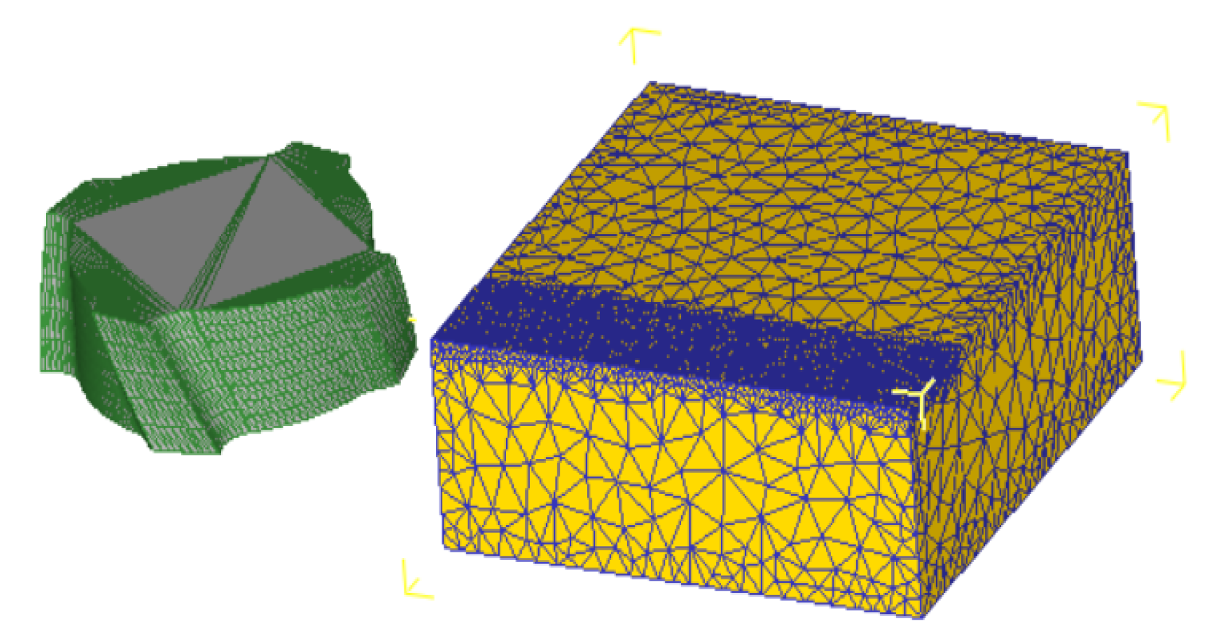
2.1. Establish Geometric Modeling of Tool and Workpiece
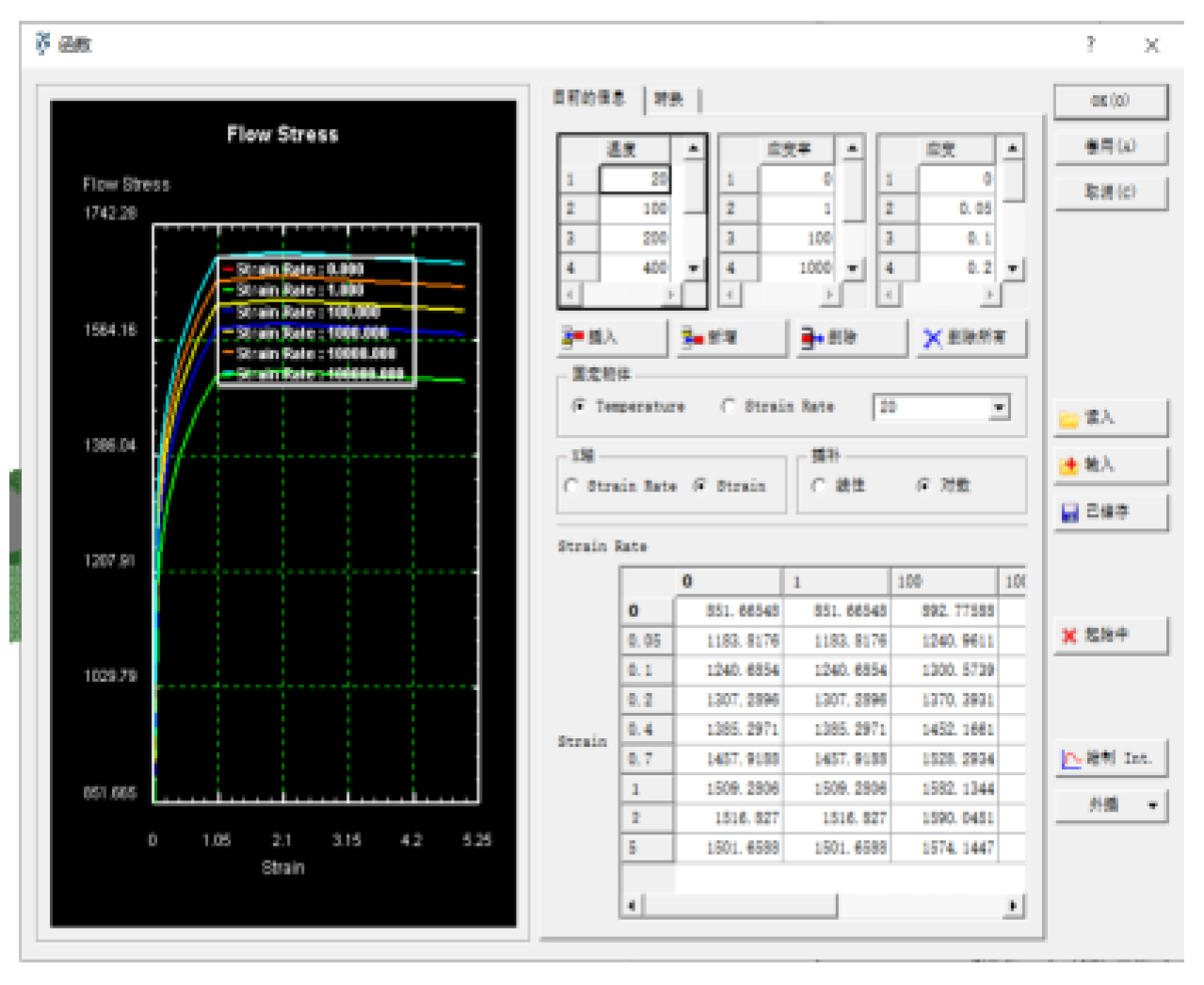
2.2. Setting up Workpiece and Tool Materials and Grid Division
2.3. Tool and Workpiece Simulation Working Condition Settings
2.4. Establishment of Tool Wear Prediction Model for Ordinary Milling
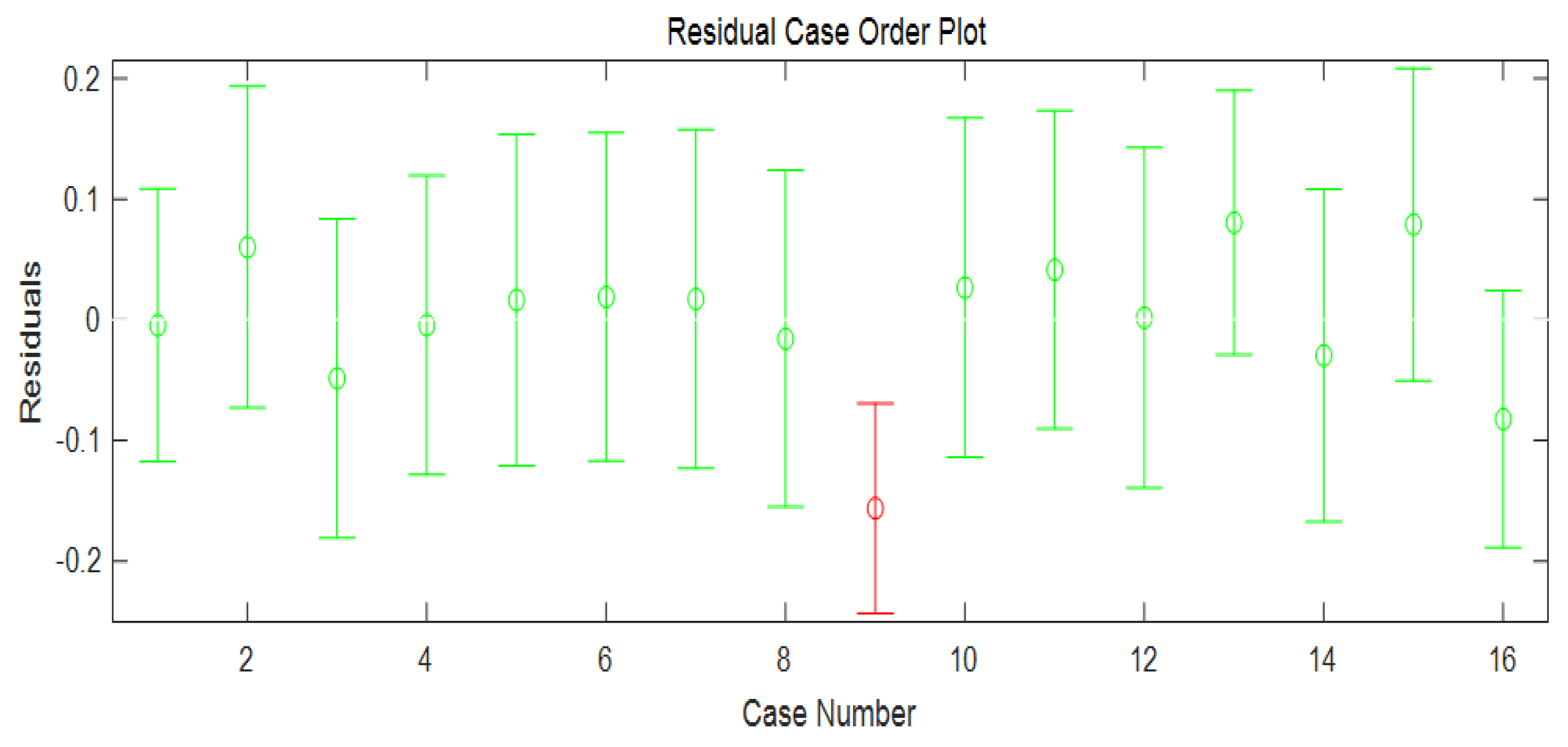
2.5. Linear Regression Significance Test
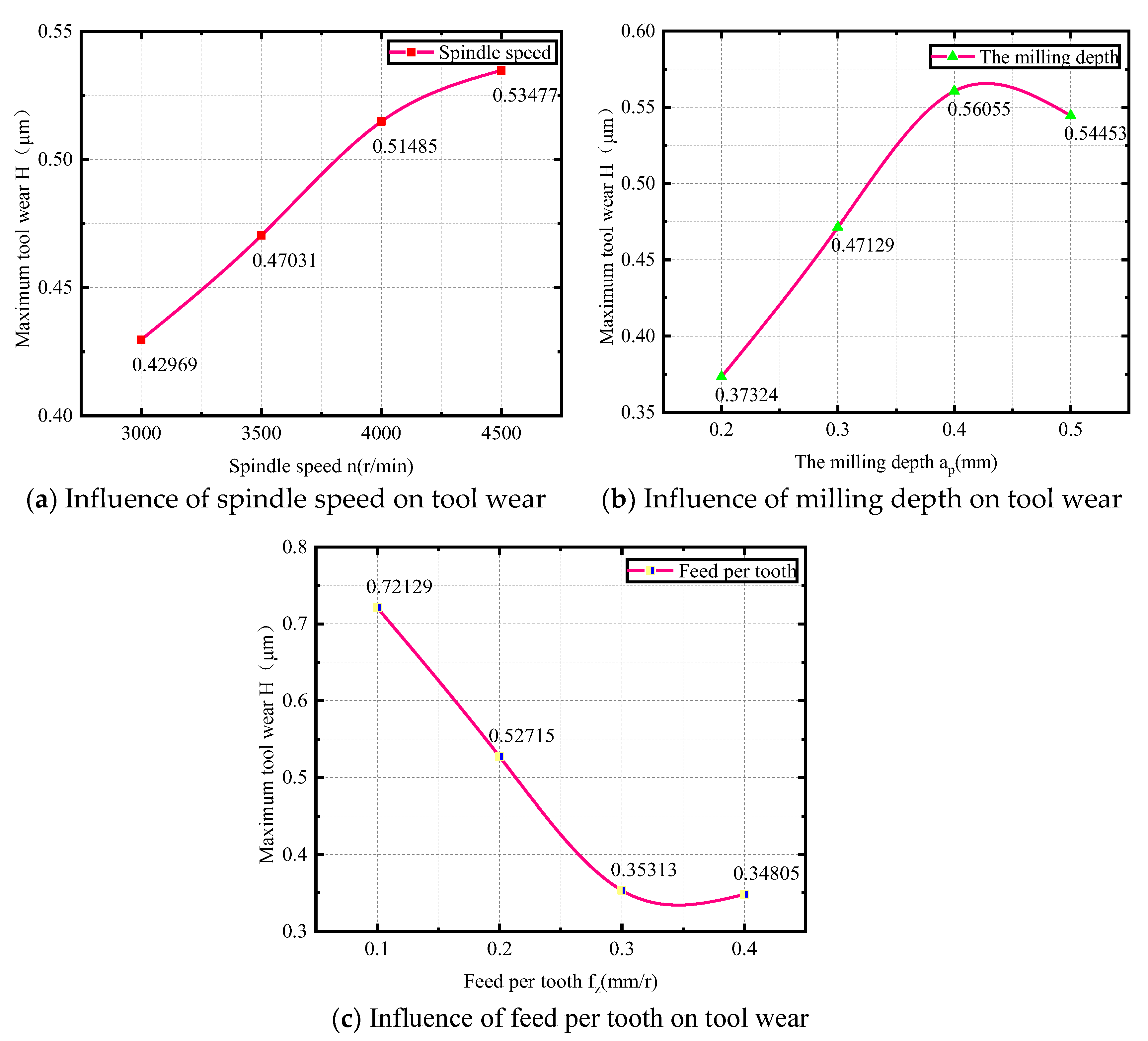
2.6. Analysis of Impact Patterns
3. Comparative Analysis of Ultrasonic Vibration Milling and Ordinary Milling
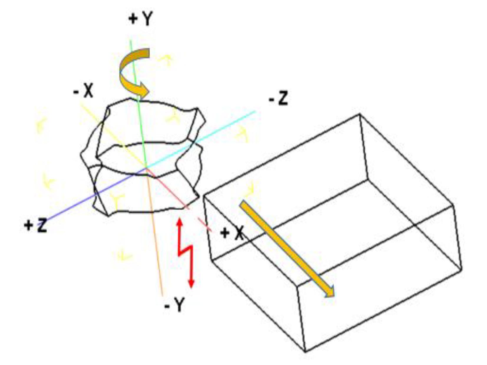
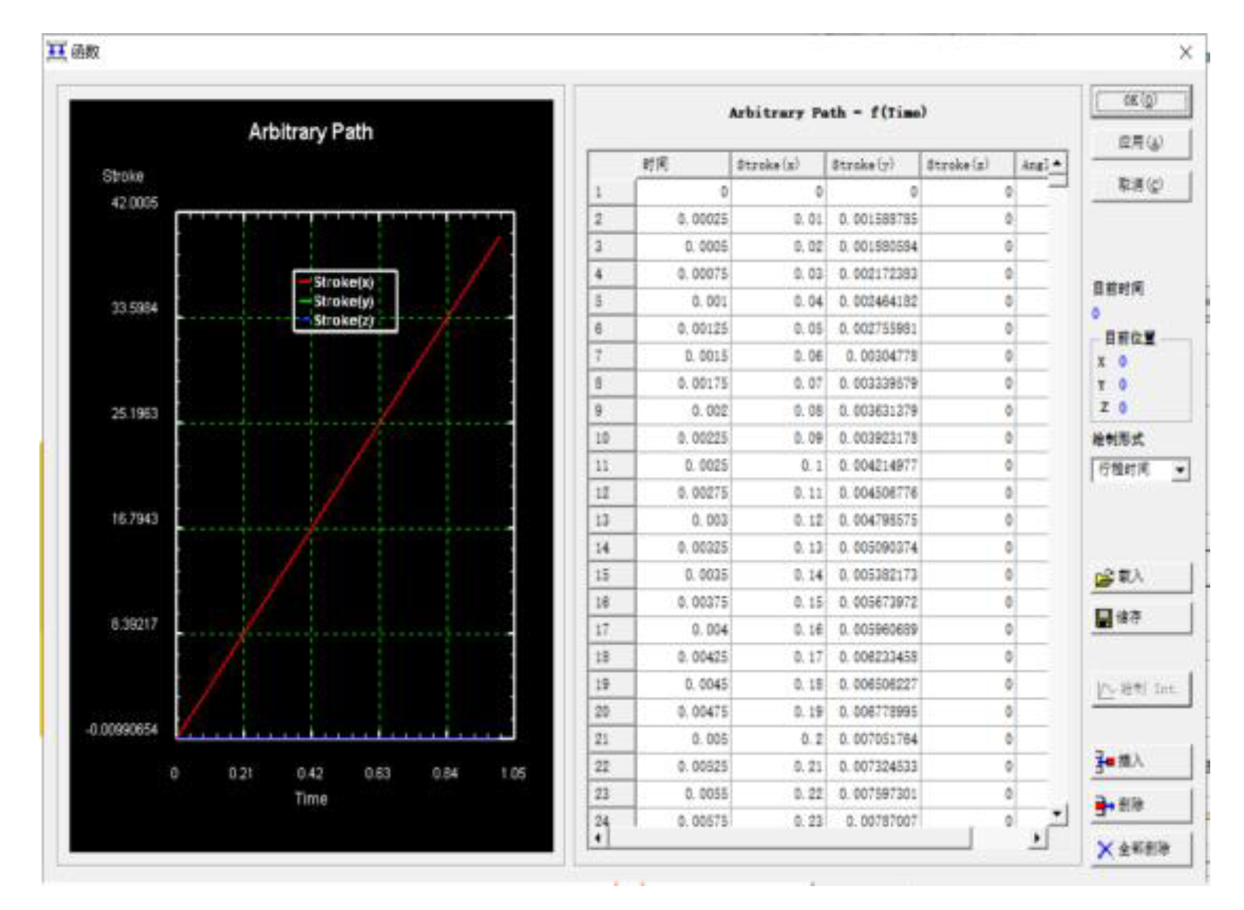
3.1. Establishment of GH4169 Model for Cemented Carbide Vibration Milling
3.2. Comparison of Results between Axial Ultrasonic Vibration Milling and Ordinary Milling
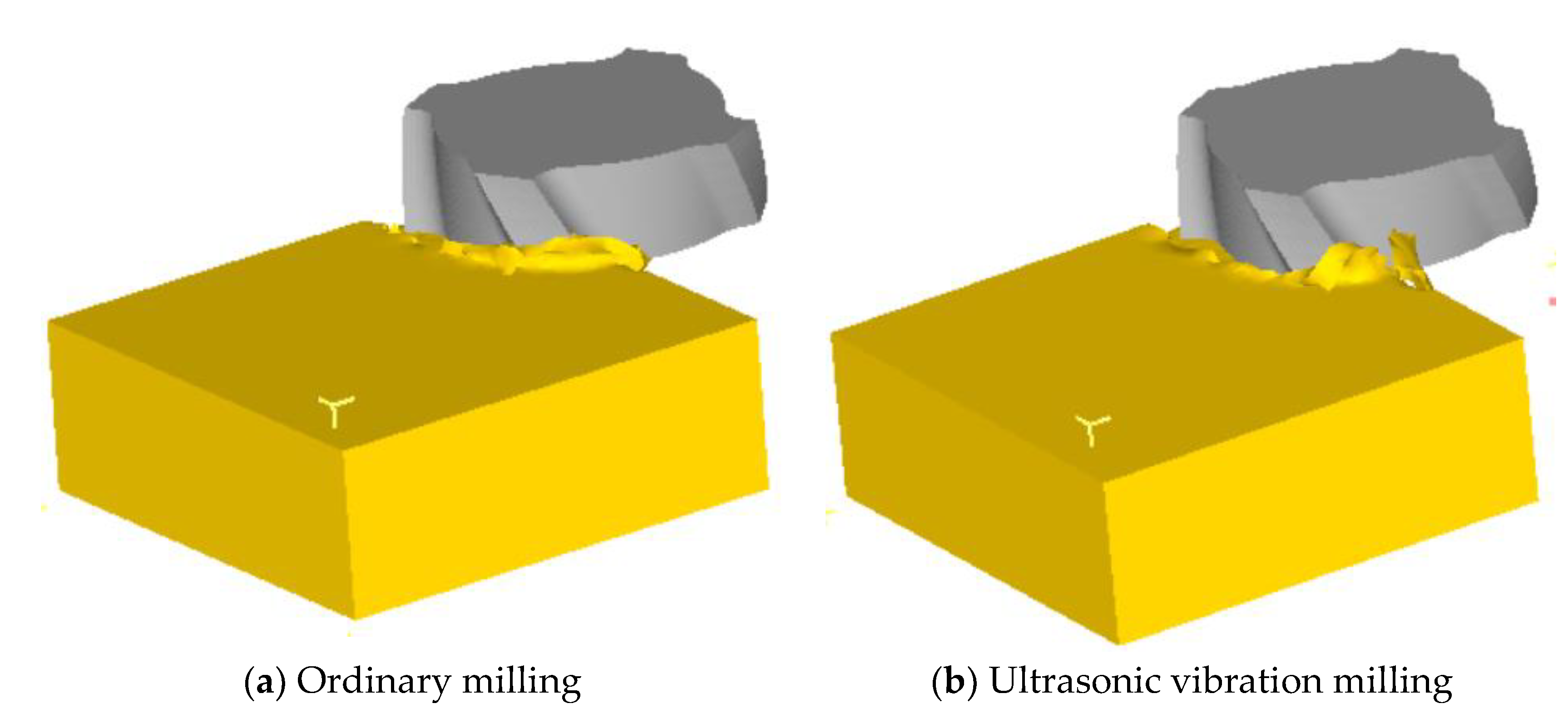
3.2.1. Comparison of Chip Shapes
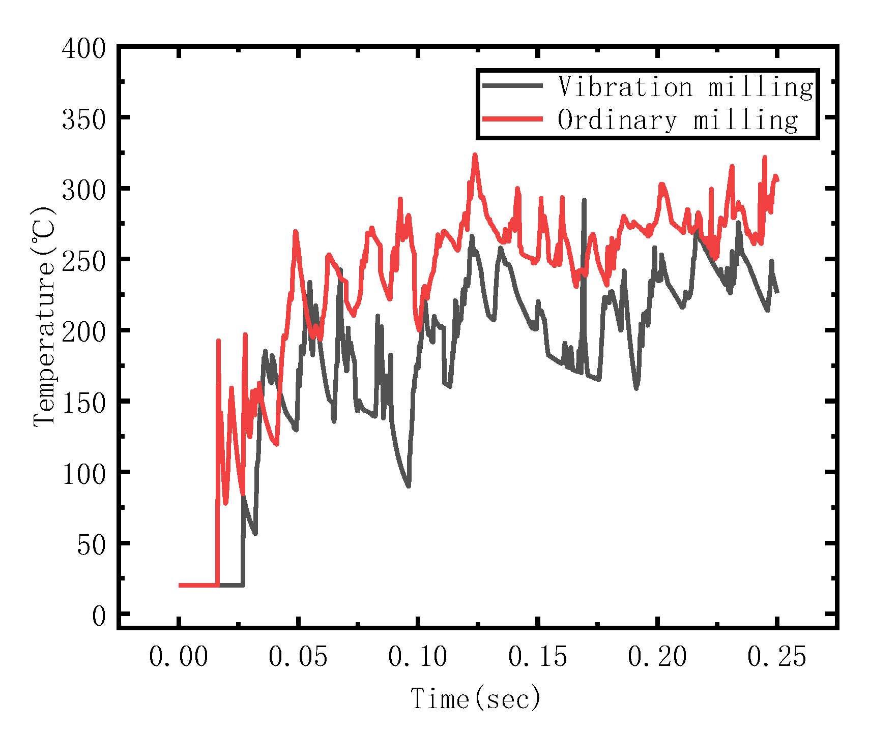
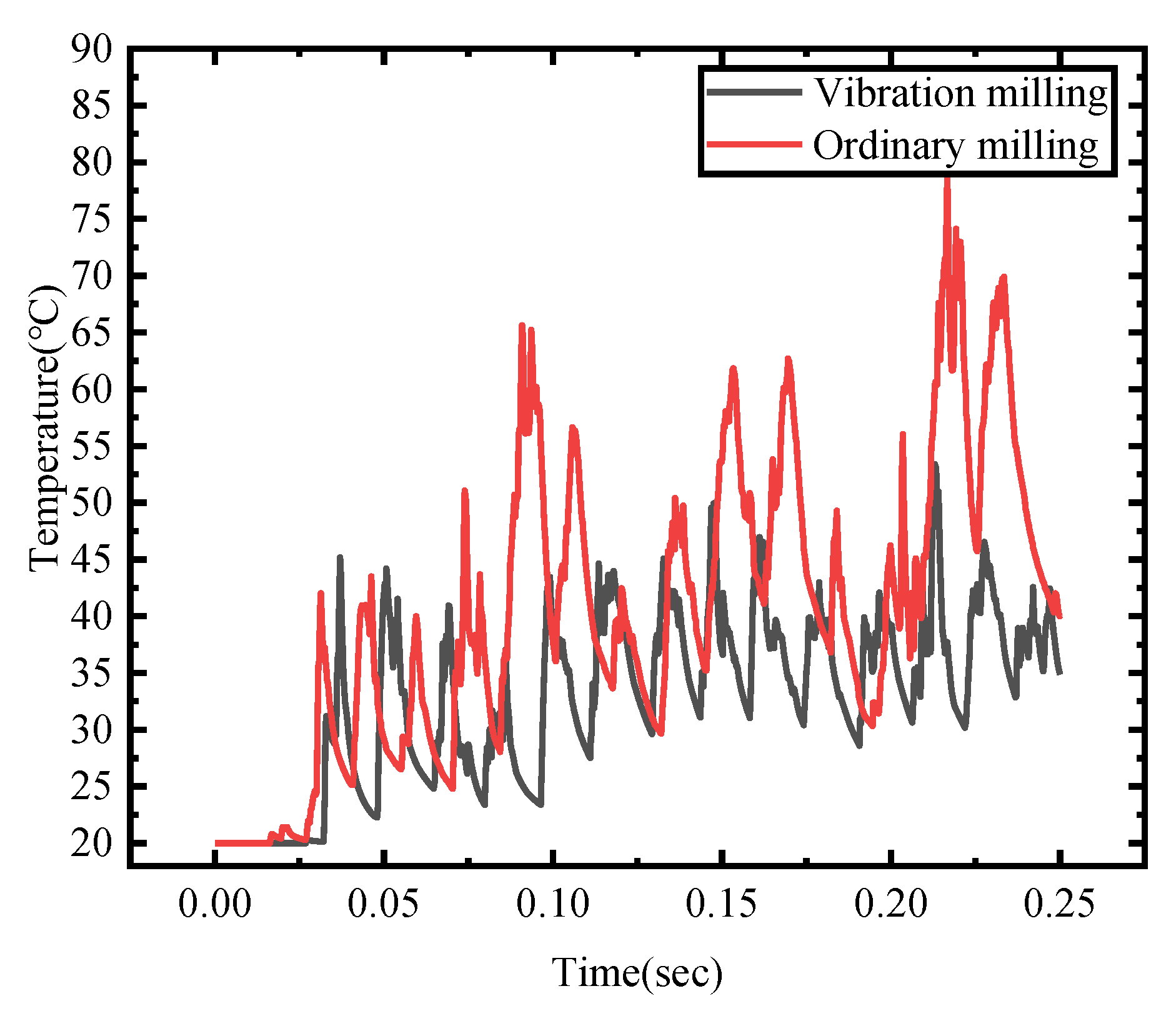
3.2.2. Temperature Comparison in Milling Area
3.2.3. Tool Temperature Comparison
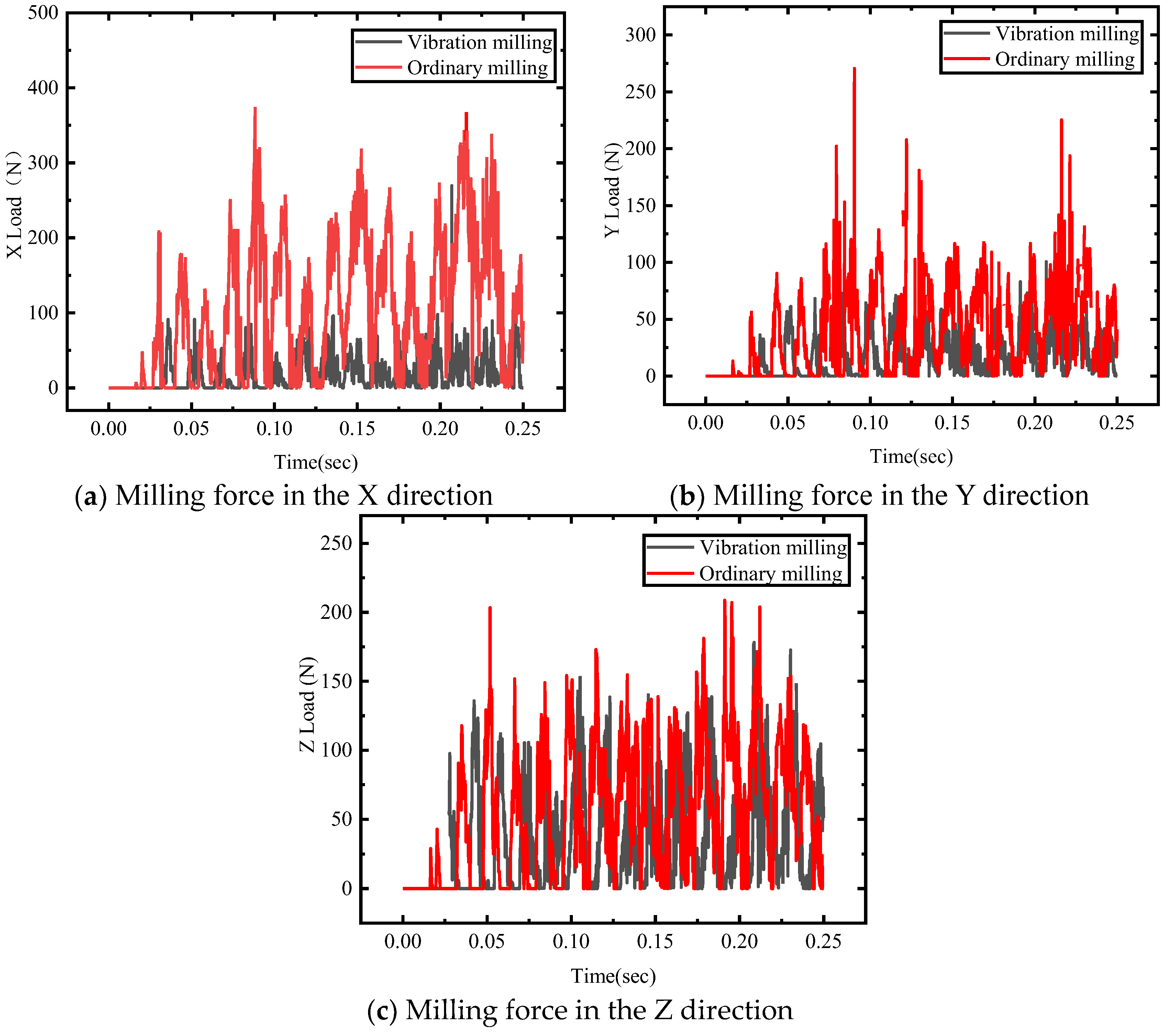
3.2.4. Comparison of Three Way Milling Forces
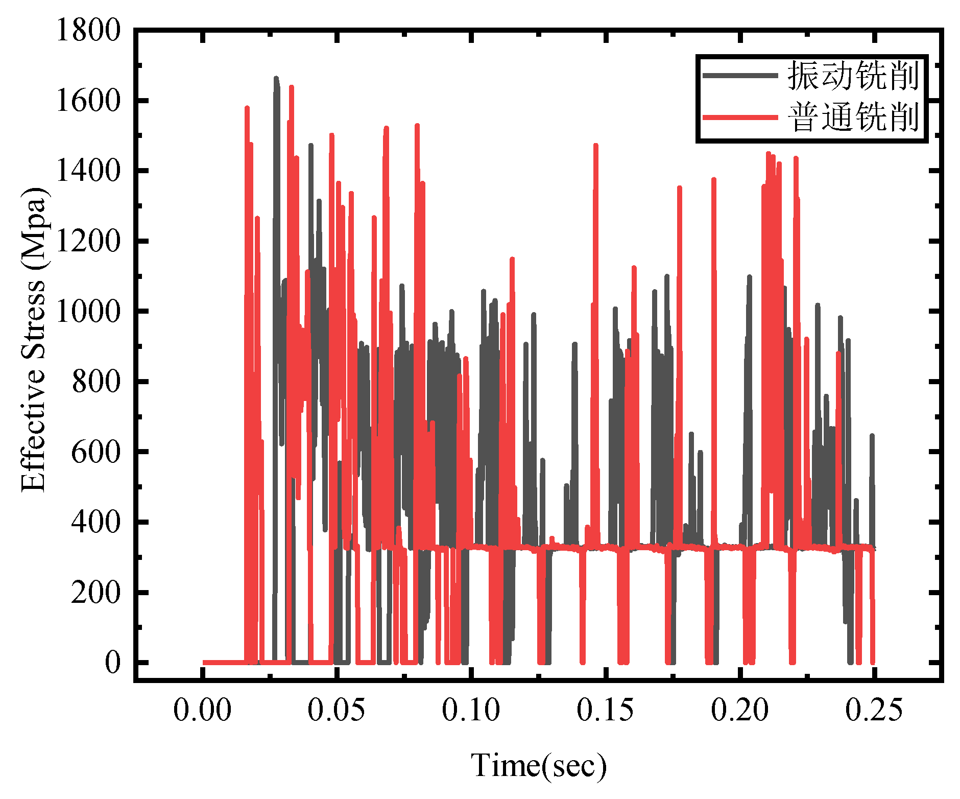
3.2.5. Comparison of Surface Stress of Workpieces
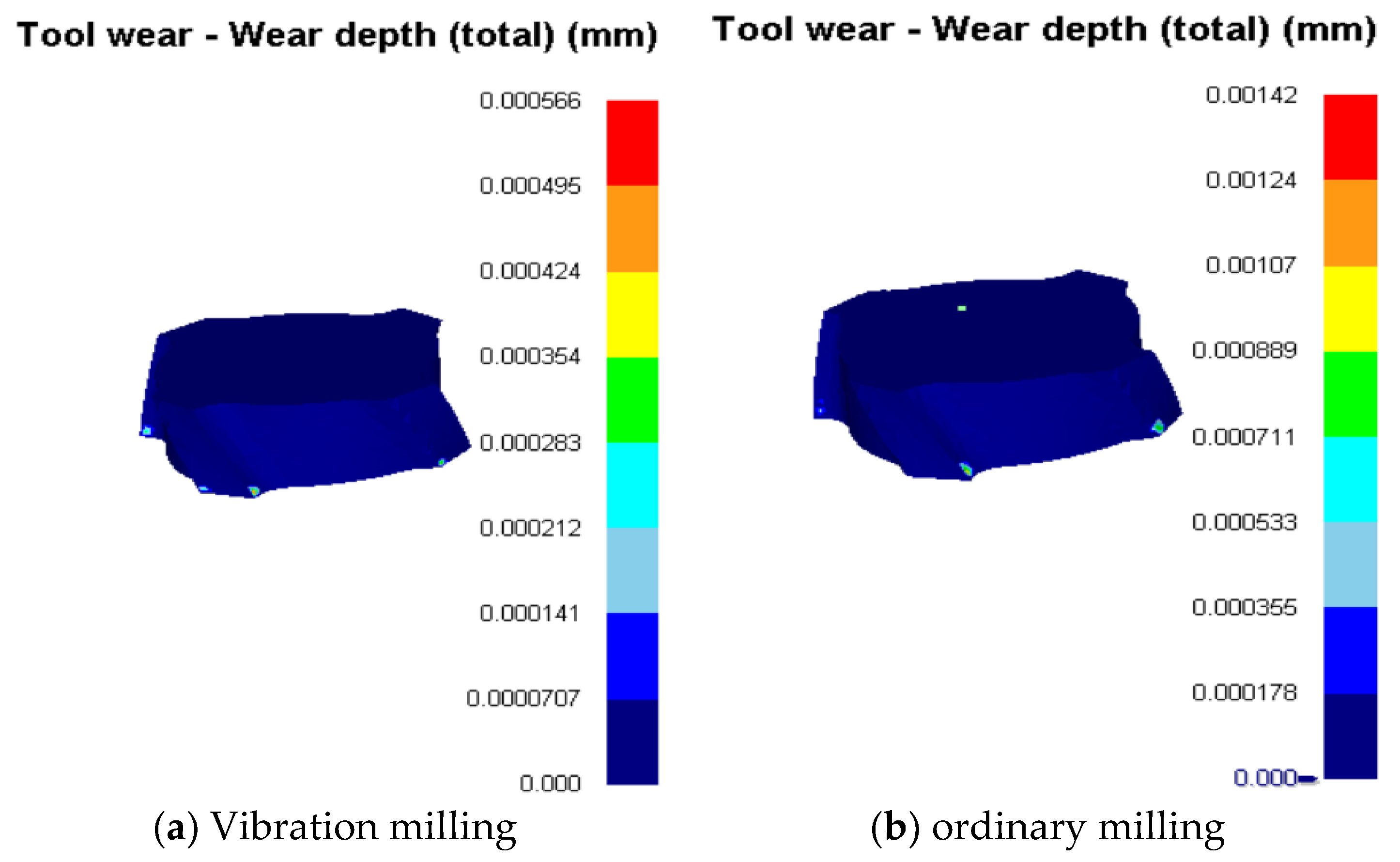
3.2.6. Comparison of Tool Wear
4. Effect of Coating Materials on Tool Wear in GH4169 Milling
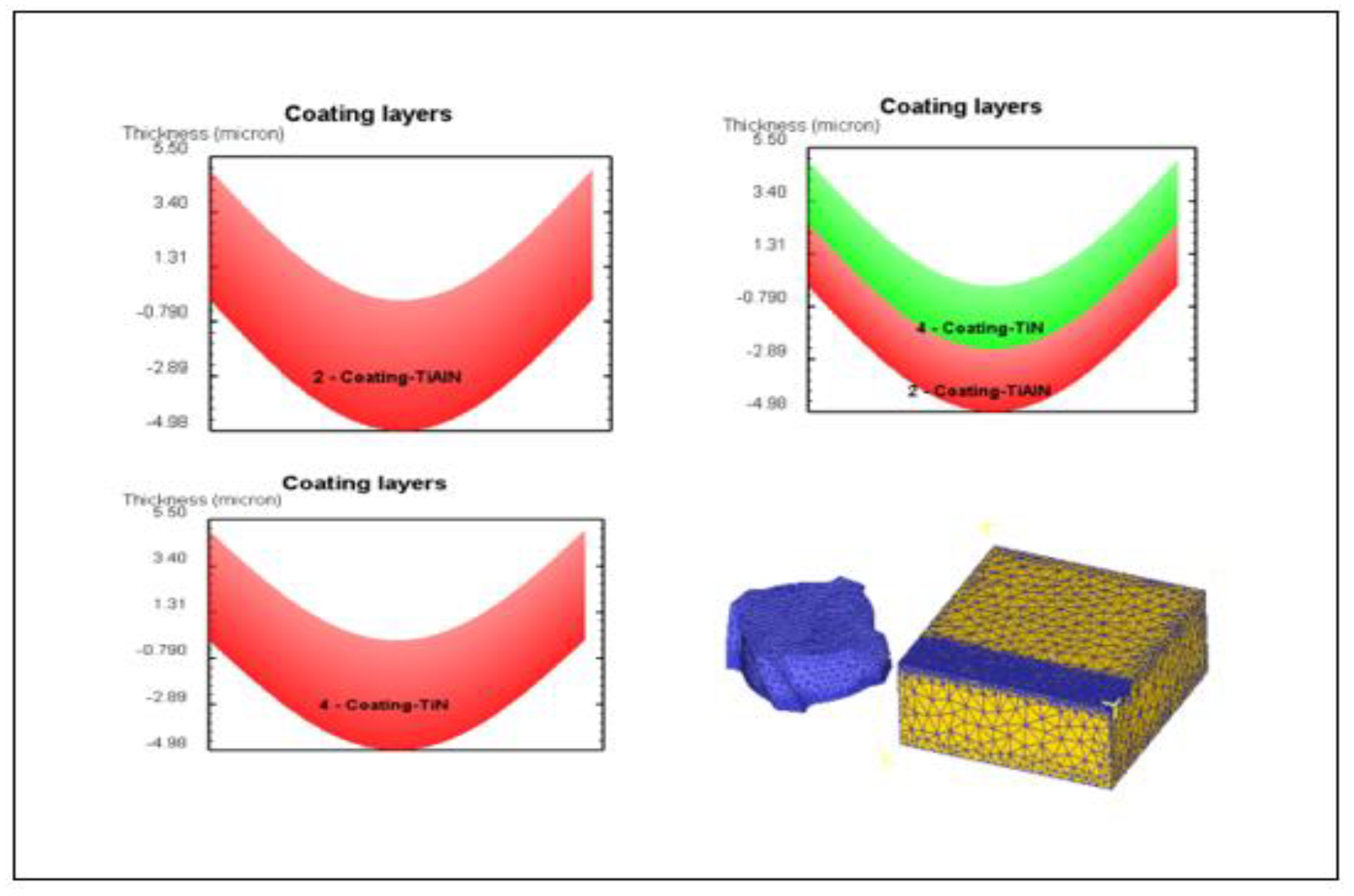
4.1. Establishment of Simulation Model for GH4169 Milling with Coated Tools
4.2. Analysis of Simulation Results
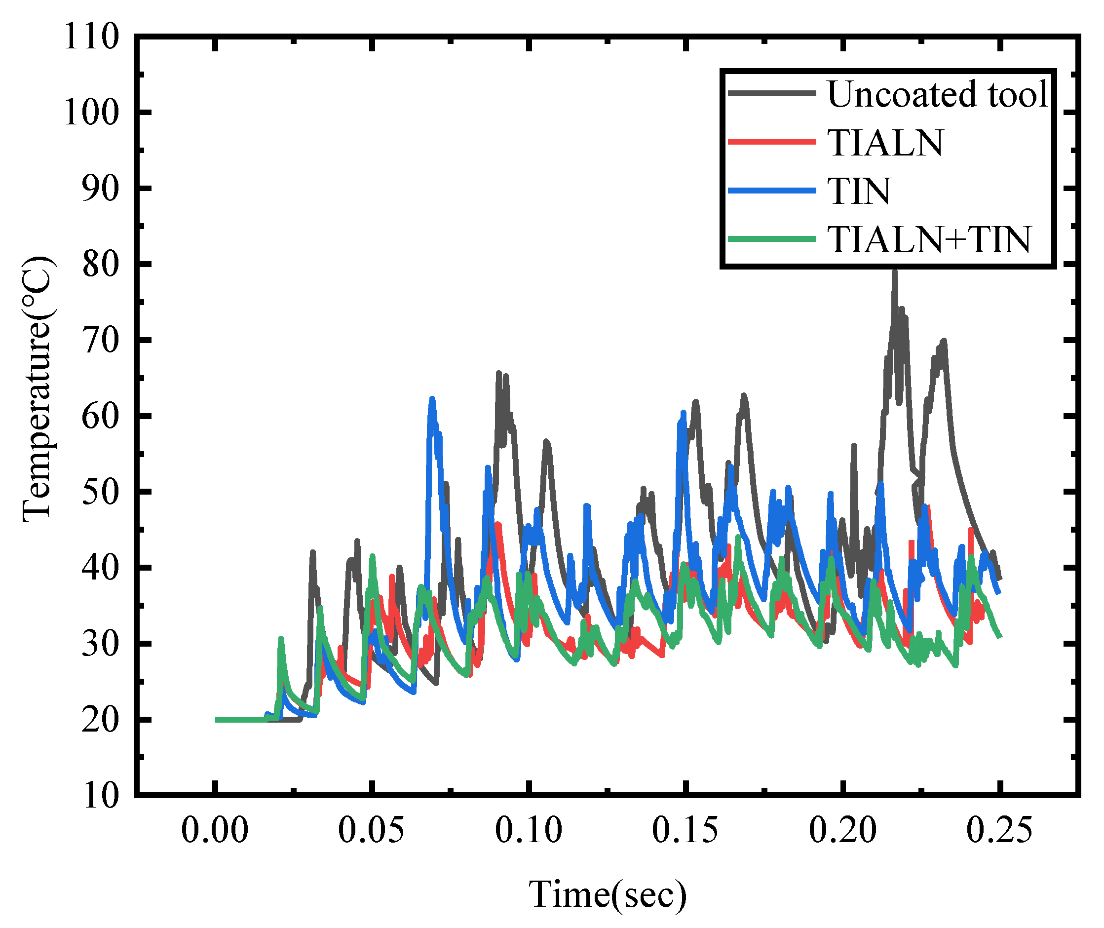
4.2.1. Temperature Changes of Cutting Tools with Different Coating Types
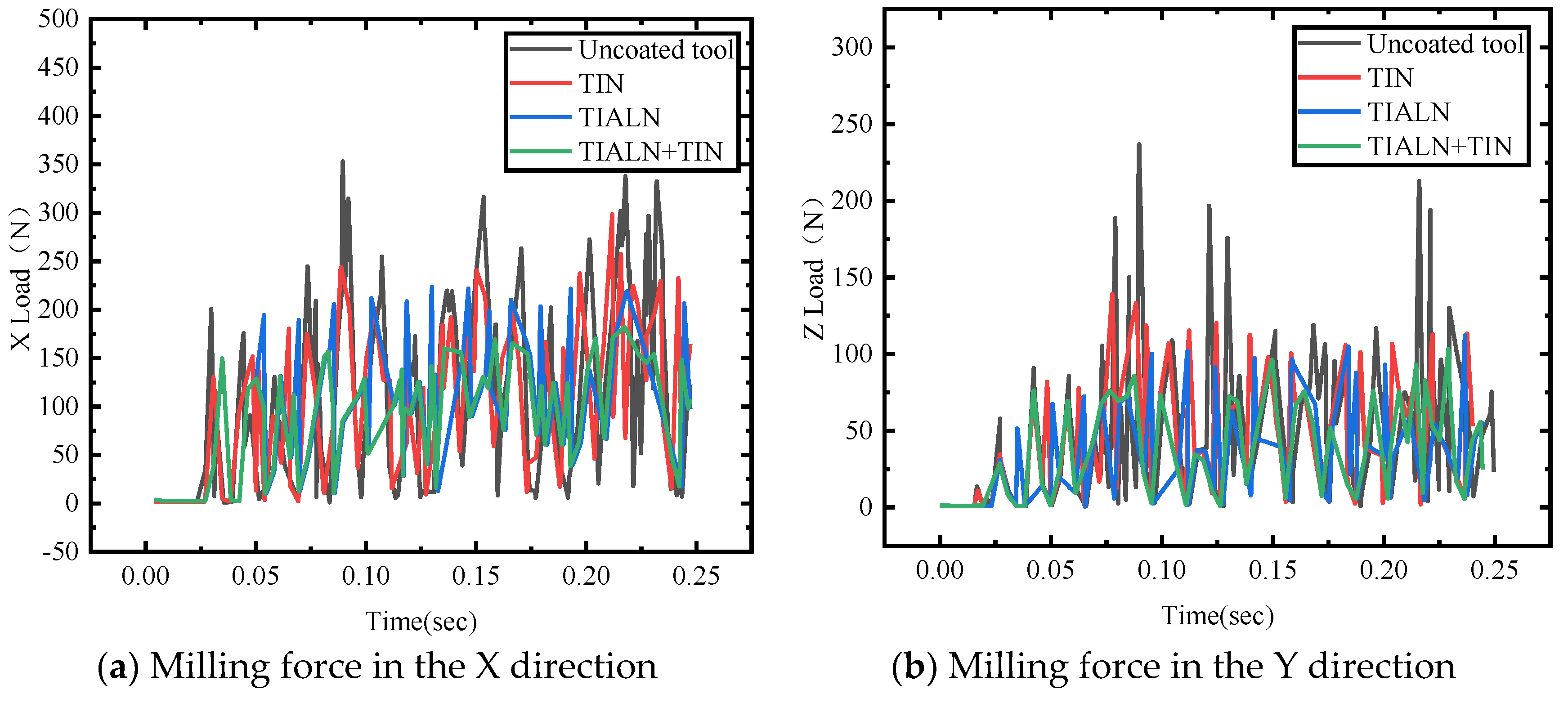
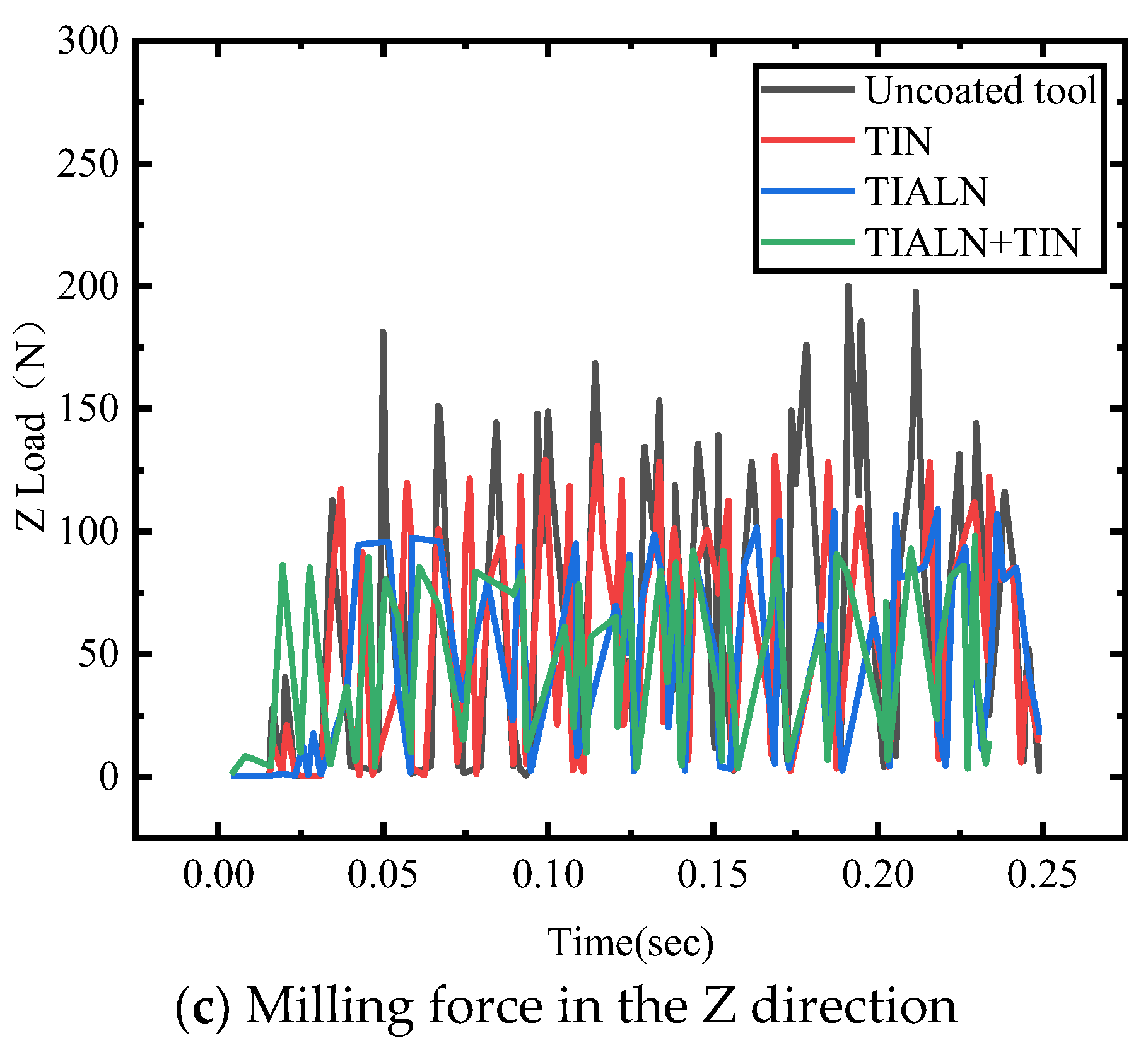
4.2.2. Changes in Milling Force of Different Coating Types of Cutting Tools
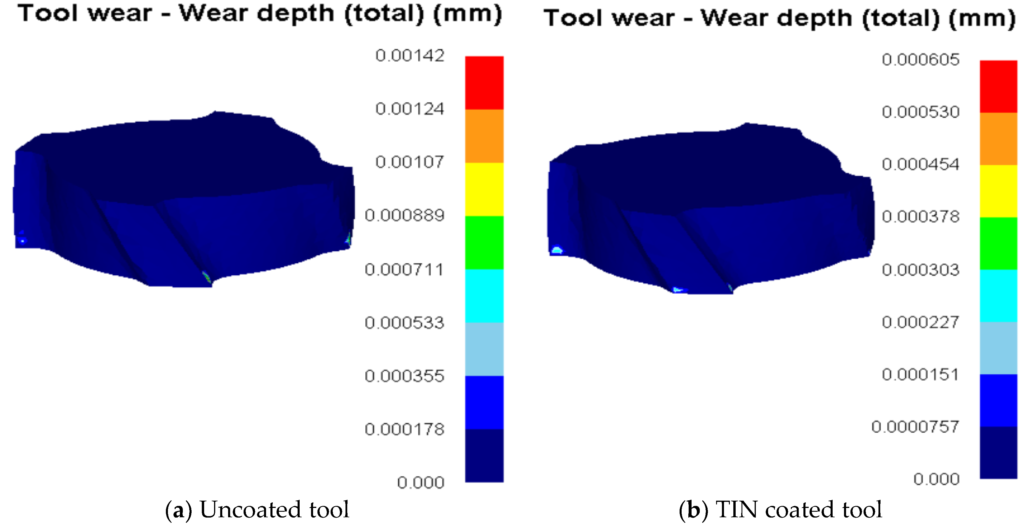
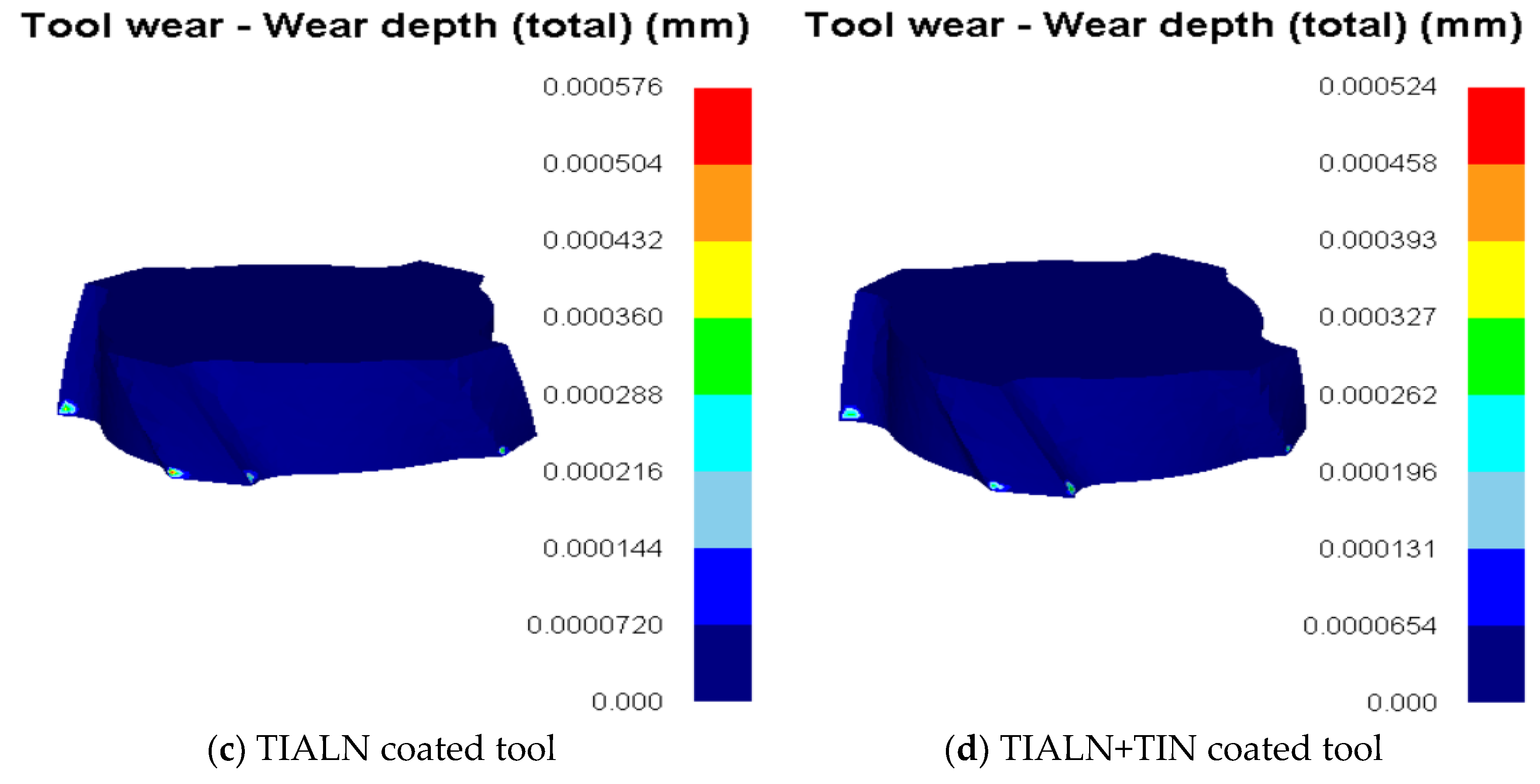
4.2.3. Comparison of Tool Wear of Different Coating Types
5. Conclusion
Funding
Availability of Data and Materials
Acknowledgments
Conflicts of Interest
Ethics Declarations
References
- Paulonis, D.F.; Oblak, J.M.; Duvall, D.S. Precipitation in Nickel-BaseAlloy718. Transactions of the ASM 1969, 62, 611–622. [Google Scholar]
- Lingenfelter, A. Welding of Inconel Alloy 718: A Historical Overview. Superalloy 1989, 718, 673–683. [Google Scholar]
- De Bartolomeis, A.; Newman, S.T.; Jawahir, I.S.; et al. Future research directions in the machining of Inconel 718. Journal of Materials Processing Technology 2021, 297, 117260. [Google Scholar] [CrossRef]
- ASM Specialty Handbook: Nickel, Cobalt, and Their Alloys; ASM International, 2000.
- Ma, J.; Jia, Z.; He, G.; et al. Influence of cutting tool geometrical parameters on tool wear in high-speed milling of Inconel 718 curved surface. Proceedings of the Institution of Mechanical Engineers, Part B: Journal of Engineering Manufacture 2019, 233, 18–30. [Google Scholar] [CrossRef]
- Fan, Y.H.; Wang, T.; Hao, Z.P.; et al. Research on tool wear based on multi-scale simulation in high speed cutting Inconel718. Archives of Civil and Mechanical Engineering 2018, 18, 928–940. [Google Scholar] [CrossRef]
- Qiao, Y.; Ai, x.; Liu, Z.; Zhao, J. Experimental Investigation into Milling of Nickel-Based Powder Metallurgy Superalloy with Coated Tools. Journal of South China University of Technology (Natural Science Edition) 2010, 38, 83–88. [Google Scholar] [CrossRef]
- Qiao, Y.; Ai, x.; Zhao, J.; Liu, Z. Failure Mechanism of Coated Carbide Tools in Milling of Nickel-base Powder Metallurgy Superalloy. Journal of Beijing University of Technology 2011, 37, 1–6. [Google Scholar]
- Liu, Y.; Liu, G. Analysis of milling tool for Nickel-based superalloy. China Water Transport 2008, 8, 170–171. [Google Scholar] [CrossRef]
- Leone, C.; D’Addona, D.; Teti, R. Tool wear modelling through regression analysis and intelligent methods for nickel base alloy machining. CIRP Journal of Manufacturing Science and Technology 2011, 4, 327–331. [Google Scholar] [CrossRef]
- Zhou, J.; Han, R.D. The Investigation of Tool Wear in High Speed Cutting INCONEL718. Applied Mechanics and Materials 2010, 33, 347–350. [Google Scholar] [CrossRef]
- Oliveira, A.R.F.; Da Silva, L.R.R.; Baldin, V.; et al. Effect of tool wear on the surface integrity of Inconel 718 in face milling with cemented carbide tools. Wear 2021, 476, 203752. [Google Scholar] [CrossRef]
- D’addona, D.M.; Raykar, S.J.; Narke, M.M. High speed machining of Inconel 718: tool wear and surface roughness analysis. Procedia CIRP 2017, 62, 269–274. [Google Scholar] [CrossRef]
- Attanasio, A.; Ceretti, E.; Rizzuti, S. 3D finite element analysis of tool wear in machining. CIRP Annals - Manufacturing Technology 2008, 57, 61–64. [Google Scholar] [CrossRef]
- Martynov, V.V.; Martynov, P.V. Automation and Modern Technologies. 2013, 4, 7–18. [Google Scholar]
- Thakur, D.G.; Ramamoorthy, B.; Vijayaraghavan, L. Some investigations on high speed machining of aerospace material Inconel 718 using multicoated carbide inserts. Materials and Manufacturing Processes 2012, 27, 1066–1072. [Google Scholar] [CrossRef]
- Yen, Y.C.; Altan, T. Estimation of Tool Wear in Orthogonal Cutting Using the Finite Element Analysis. Journal of Materials Processing Technology 2004, 82–91. [Google Scholar] [CrossRef]
- Xie, L.J. 2D FEM Estimate of Tool Wear in Turning Operation. Wear 2005, 1479–1490. [Google Scholar] [CrossRef]
- Umbrello, D.; Filice, L.; Micari, F. Prediction of Tool Wear Progress in Machining of Carbon Steel using different Tool Wear Mechanisms. Int JMater Form 2008, 1, 571–574. [Google Scholar] [CrossRef]
- Attanasio, A.; Umbrello, D. Abrasive and diffusive tool wear FEM simulation. Int J Mater Form 2009, 2, 543–46. [Google Scholar] [CrossRef]
- Zheng, M.; Fan, Y. An Overview of Tool Friction and Wear Behavior in High-speed Machining-typical Difficult-to-cut Material. Journal of Harbin University of Science and Technology 2011, 16, 22–30. [Google Scholar] [CrossRef]
- He, Y.; Zhou, Z.; Zou, P.; et al. Study of ultrasonic vibration–assisted thread turning of Inconel 718 superalloy. Advances in Mechanical Engineering 2019, 11, 1687814019883772. [Google Scholar] [CrossRef]
- Mou, W.; Zhu, S. Vibration, tool wear and surface roughness characteristics in turning of Inconel 718 alloy with ceramic insert under LN2 machining. Journal of the Brazilian Society of Mechanical Sciences and Engineering 2020, 42, 1–12. [Google Scholar] [CrossRef]
- Sharman, A.; Dewes, R.C.; Aspinwall, D.K. Too1 life when high speed bal1 nose end milling Inconel 718. Journal of Materials Processing Technology 2001, 118, 29–35. [Google Scholar] [CrossRef]
- Wang, Q. Research and application of functional principal component analysis and functional linear regression model. Dissertation, Chongqing Technology and Business University, 2020. [Google Scholar]
- Ma, Y.; Yue, Y. Research on Surface Roughness Prediction Model of T-itanium Alloy TC25 Milling. Manufacturing Technology & Machine Tool 2020, 141–145. [Google Scholar] [CrossRef]
- Liu, A. SPSS basic analysis tutorial; Peking University Press: Beijing, 2014. [Google Scholar]
- Peng, D. Prediction of Milling Process and Analysis of Surface Quality for TC4. Dissertation, Tianjin University, 2012. [Google Scholar]
- Yang, Y. Numerical Simulation and Experimental Study on Axial Ultrasonic Vibration Assisted Milling of Titanium Alloy. Dissertation, Nanjing University of Science and Technology, 2021. [Google Scholar]
- Liu, Z.; Zhang, C.; Ren, J. Dry cutting technology and its application; China Machine Press: Beijing, China, 2005. [Google Scholar]
| Diameter | Tooth number | Front Angle | back Angle | helix Angle | radius of the tool |
|---|---|---|---|---|---|
| 10mm | 4 | 8° | 12° | 30° | 1mm |
| Spindle speed n(r/min) | Cutting depth ap(mm) | Feed per tooth fz(mm/r) | Tool wear amountH(μm) | |
|---|---|---|---|---|
| 1 | 3000 | 0.2 | 0.1 | 0.557 |
| 2 | 3000 | 0.3 | 0.2 | 0.499 |
| 3 | 3000 | 0.4 | 0.3 | 0.343 |
| 4 | 3000 | 0.5 | 0.4 | 0.351 |
| 5 | 3500 | 0.2 | 0.2 | 0.387 |
| 6 | 3500 | 0.3 | 0.1 | 0.778 |
| 7 | 3500 | 0.4 | 0.4 | 0.349 |
| 8 | 3500 | 0.5 | 0.3 | 0.444 |
| 9 | 4000 | 0.2 | 0.3 | 0.208 |
| 10 | 4000 | 0.3 | 0.4 | 0.323 |
| 11 | 4000 | 0.4 | 0.1 | 1.01 |
| 12 | 4000 | 0.5 | 0.2 | 0.645 |
| 13 | 4500 | 0.2 | 0.4 | 0.309 |
| 14 | 4500 | 0.3 | 0.3 | 0.363 |
| 15 | 4500 | 0.4 | 0.2 | 0.718 |
| 16 | 4500 | 0.5 | 0.1 | 0.898 |
| A(Speed) | B(The millin depth) | C(Feed per tooth) | |
|---|---|---|---|
| K1 | 1.7500 | 1.4610 | 3.2430 |
| K2 | 1.9580 | 1.9630 | 2.2490 |
| K3 | 2.1860 | 2.4200 | 1.3580 |
| K4 | 2.2880 | 2.3380 | 1.3320 |
| k1 | 0.4375 | 0.3653 | 0.8108 |
| k2 | 0.4895 | 0.4908 | 0.5623 |
| k3 | 0.5465 | 0.6050 | 0.3395 |
| k4 | 0.5720 | 0.5845 | 0.3330 |
| RF | 0.1345 | 0.2398 | 0.4778 |
| 主次顺序 | fz>ap>n | ||
| Coating types | TIALN | TIN |
| Hardness value(HV) | 3300 | 2300 |
| The coefficient of friction(N/sec/mm/C) | 0.4 | 0.49 |
| Coefficient of heat conduction | 10 | 23 |
Disclaimer/Publisher’s Note: The statements, opinions and data contained in all publications are solely those of the individual author(s) and contributor(s) and not of MDPI and/or the editor(s). MDPI and/or the editor(s) disclaim responsibility for any injury to people or property resulting from any ideas, methods, instructions or products referred to in the content. |
© 2023 by the authors. Licensee MDPI, Basel, Switzerland. This article is an open access article distributed under the terms and conditions of the Creative Commons Attribution (CC BY) license (http://creativecommons.org/licenses/by/4.0/).


