Preprint
Article

Coarse and Fine Two-Stage Calibration Method for Enhancing the Accuracy of Inverse Finite Element Method

Altmetrics

Downloads

108

Views

12

Comments

0

A peer-reviewed article of this preprint also exists.

This version is not peer-reviewed

Submitted:

18 May 2023

Posted:

19 May 2023

You are already at the latest version

Alerts
Abstract
The inverse finite element method (iFEM) is a novel method for reconstructing the full-field displacement of structures by discrete measurement strain. In practical engineering applications, the accuracy of iFEM is reduced due to the positional offset of strain sensors during installation, and errors in structural installation. Therefore, coarse and fine two-stage calibration (CFTSC) method is proposed to enhance the accuracy of the reconstruction of structures. Firstly, the coarse calibration is based on a single-objective particle swarm optimization algorithm to optimize the displacement-strain transformation matrix related to the sensor position. Secondly, as selecting different training data can affect the training effect of self-constructed fuzzy networks, this paper proposes to screen the appropriate training data based on residual analysis. Finally, the experiments of the wing integrated antenna structure verify the efficient of the method on the reconstruction accuracy of the structural body displacement field.
Keywords: 
Subject: Engineering  -   Mechanical Engineering

1. Introduction

Shape sensing is significant for the safety monitoring of structures such as aircraft and radar antennas. This technology is applied in various aspects of aerospace, military and civil applications [1,2,3]. Considering that the array accuracy and electrical performance are affected by the antenna deformation [4,5,6], the shape sensing technique is significant for the antenna performance. The shape sensing method can currently be divided into two categories [7,8]: one is non-contact measurement and the other is contact measurement. Non-contact measurement is based on laser tracking, laser position sensor method to measure displacement directly and real-time measurement is difficult to achieve due to the high requirements for the measurement environment and measurement instruments in practical engineering applications. The contact measurement method is used to calculate the deformation and displacement of the structure by strain sensors to obtain strain information, which has promising application in practical engineering [9,10,11].
The methods for reconstructing the structural displacement field based on strain information are divided into: KO displacement theory, modal method and iFEM. Ko displacement theory establishes a mathematical model for the strain according to the primary or secondary distribution and combines it with the shape function to calculate the displacement [12,13]. However, this method is only applicable to the problem of reconstructing the unidirectional displacement field. The modal method is to measure the strain values and strain modes at specified locations, solving for the modal coordinates of each order mode, and then obtain the displacement field of the structure [14,15]. But this method requires a high precision physical model and not applicable to the deformation reconstruction of structures under high frequency excitation response. The iFEM was proposed by Tessler and Spangler [16,17] with the most widespread and promising applications among the three methods. This method discounts the material properties of the structure and the information of the applied load, with the advantages of high reconstruction accuracy and rapid reconstruction of the displacement field. The iFEM is based on the least-squares variational principle. The strain values are measured experimentally and a mathematical model of strain-displacement is established. Kefal and Oterkus et al [18] proposed an inverse finite element model with a quadrilateral cell. Comparing to the triangular cell, the generation of singular matrices in the inverse operation is avoided due to the increase of angular degrees of freedom in the z-direction, preventing the shear self-locking phenomenon of the shell structure when reconstructing the deformation field. Gherlone et al. [19,20] proposed to paste fiber brag grating (FBG) sensors on the surface of a Timoshenko beam to obtain the shape sensing of the beam structure in transverse shear, tension, bending, and torsional deformation. Cerracchio et al. [21] proposed to combine in the original inverse finite element formulation with the refined Zigzag theory, which is applicable to the deformation monitoring of multilayer composites and sandwich structures. Bao et al. [22] proposed an inverse finite element model using a univariate to optimize the number of sensors installed on the Timoshenko beam. Niu et al. [23] proposed the inverse scaled boundary element to model the Kirchhoff plates structures reconstruction, and the method achieves the 3D deformation reconstruction through the strain information on the single-layer surface of the plate structure.
In practical engineering, the measurement errors due to strain transducer installation offset and structural body errors can reduce the reconstruction accuracy of the iFEM. To solve the problem, Zhao [24,25] proposed a particle swarm optimization algorithm to determine the sensor layout locations. Pan [26] proposed a method to calibrate strains by mapping experiments using fuzzy networks to measure strain values. However, structural errors can greatly affect the calibration results of this method. Fu et al. [27] proposed the method that combines support vectors with fuzzy networks to correct for strain errors. The drawback of this method is the lack of a large amount of experimental working condition data, which will have an impact on the training of the fuzzy network. To address the problem of the effect of small sample size on reconstruction accuracy, Xu et al. [28] proposed a two-step calibration method, but this method is limited to the reconstruction displacement accuracy at the maximum deformation position, and the reconstruction accuracy at the rest of the positions is not as accurate. Li et al. [29] determined the layout location of sensors based on multi-objective particle swarm optimization algorithm. The fuzzy network calibration method for the small sample problem was proposed by Li et al. [30], which improves the reconstructed accuracy of the whole displacement field effectively. However, when strain sensors are artificially installed to measure strain values, the offset in the installation position of the sensor increases the error in the reconstruction of the deformation field.
For improving the accuracy of reconstructed displacement field, this paper proposes a CFTSC method. Firstly, the coarse calibration method is based on a single-objective particle swarm optimization algorithm to correct the error of the displacement-strain matrix due to the offset of the sensor position installation. After the coarse calibration, the fine calibration of the system error based on the self-constructed fuzzy network is continued to further improve the accuracy of the reconstructed displacement field. Secondly, since a suitable training set can improve the training effect of self-constructed fuzzy networks, this paper proposes to screen suitable training data based on residual analysis. All samples are fitted with NURBS curves to obtain the residual value of each sample point, and the samples are classified according to the residual value of each sample, from which suitable training data are screened.
The sections of this paper are described as follows. In Section 2, the theoretical framework of beam iFEM is described. In Section 3, the specific method of CFTSC is introduced. In Section 4, The calibration effect of the proposed CFTSC method on the displacement field is illustrated experimentally. Conclusions are given in Section 5.

2. The Framework of the Inverse Finite Element Method

The iFEM is based on the least squares function between the theoretical sectional strain e(u) and the actual sectional strain e ε . And can be expressed as:
Γ ( u ) = e ( u ) - e ε 2
The displacement d t at any position of the section can be represented by the shape function H(x) and the nodal degrees of freedom (DOF) u e .
d t = H ( x ) u e
The strain at any position of the cross-section can be obtained from Eq. (3).
e u = M ( x ) u e
where M(x) is the derivative of H(x), called the strain function matrix. By taking the derivative of u in Eq. (1), the derivative function of u is made to be zero, so that the difference Γ(u) between the theoretical strain and the actual strain is minimized. Eq. (4) is obtained.
k e u e = f μ
where k e and f μ are denoted as
k e = p = 1 6 w p k p e , k p e = l n i = 1 n [ M p T ( x i ) M p ( x i ) ] f μ = p = 1 6 w p f p e , f p e = l n i = 1 n [ M p T ( x i ) e p ε ( x i ) ]
where l denotes the unit length after reconstruction, n denotes the number of section strains on the neutral axis, x i denotes the position where the calculated section strains make, and w p denotes the weighting factor.
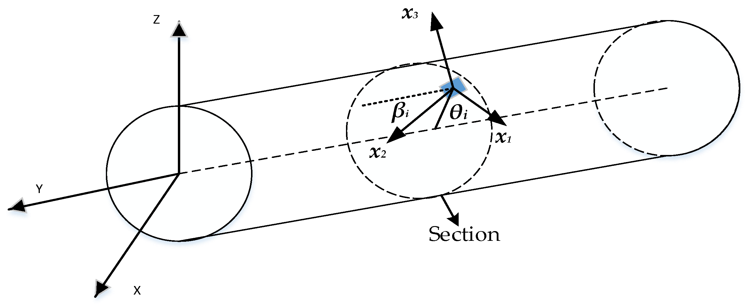
When the strain sensor layout position is determined, then the parameters x = xi, θ = θi, β = βi (i = 1,2,...6) related to the sensor position are also determined. The surface strains ε a are then calculated by Eq. (6).
ε a ( x i , θ i , β i ) = [ ( c o s 2 β - μ s i n 2 β ) , ( c o s 2 β - μ s i n 2 β ) s i n θ × r , ( c o s 2 β - μ s i n 2 β ) c o s θ × r , c o s β s i n β c o s θ , c o s β s i n β s i n θ , c o s β s i n β × r ] × [ e 1 ε ( x i ) , e 2 ε ( x i ) , e 3 ε ( x i ) , e 4 ε ( x i ) , e 5 ε ( x i ) , e 6 ε ( x i ) ] T = T × [ e 1 ε ( x i ) , e 2 ε ( x i ) , e 3 ε ( x i ) , e 4 ε ( x i ) , e 5 ε ( x i ) , e 6 ε ( x i ) ] T
where T denotes the conversion relationship between surface strain and section strain and µ denotes the Poisson ratio. r represents the outer radius of the section. As shown in the Figure 1 below.
For a section strain e i ε ( i = 1,2 , . . . , 6 ) at any position on the neutral axis can be expressed as ( e 1 ε , e 2 ε , e 3 ε , e 4 ε , e 5 ε , e 6 ε ) T=R∙[ q 1 , q 2 , q 3 , q 4 , q 5 , q 6 ]T, The matrix [ q 1 , q 2 , q 3 , q 4 , q 5 , q 6 ]T is used to represent the unknown parameters of the section strain. The specific form of the matrices R and [ q 1 , q 2 , q 3 , q 4 , q 5 , q 6 ]T are shown below.
R = [ 1 0 0 0 0 0 0 y i 1 0 0 0 0 0 0 y i 1 0 0 D y G z 0 0 0 0 0 0 0 D z G y 0 0 0 0 0 0 0 1 ]
[ q 1 , q 2 , q 3 , q 4 , q 5 , q 6 ] T = ( T × R u ) - 1 × ε a ( x i , θ i , β i ) T = ( T × [ 1 0 0 0 0 0 0 x i 1 0 0 0 0 0 0 x i 1 0 0 D y G z 0 0 0 0 0 0 0 D z G y 0 0 0 0 0 0 0 1 ] ) - 1 × ε a ( x i , θ i , β i ) T
where T=[T1,T2,T3,T4,T5,T6]T. The difference between the R matrix and the Ru matrix is that the variable yi in the R matrix is transformed into xi, xi and yi denote the position at any point along the axis x-direction or y-direction.
By substituting the obtained sectional strain e i ε   ( i = 1,2 , . . . , 6 ) into Eq. (4),
the relationship between the nodal DOF of the structural and the surface strain
can be established. This is shown in Eq. (9).
u e = ( k e ) - 1 f μ = T k × ε a ( x i ) T k = { l n × i = 1 6 [ w p M p T ( x i ) M p ( x i ) ] } - 1 × { l n × i = 1 6 [ w p M p T ( x i ) ] R ( T × R u ) - 1 ] }
where the matrix Tk is called the displacement-strain transformation matrix, which is determined by the position of the strain sensors after installation.
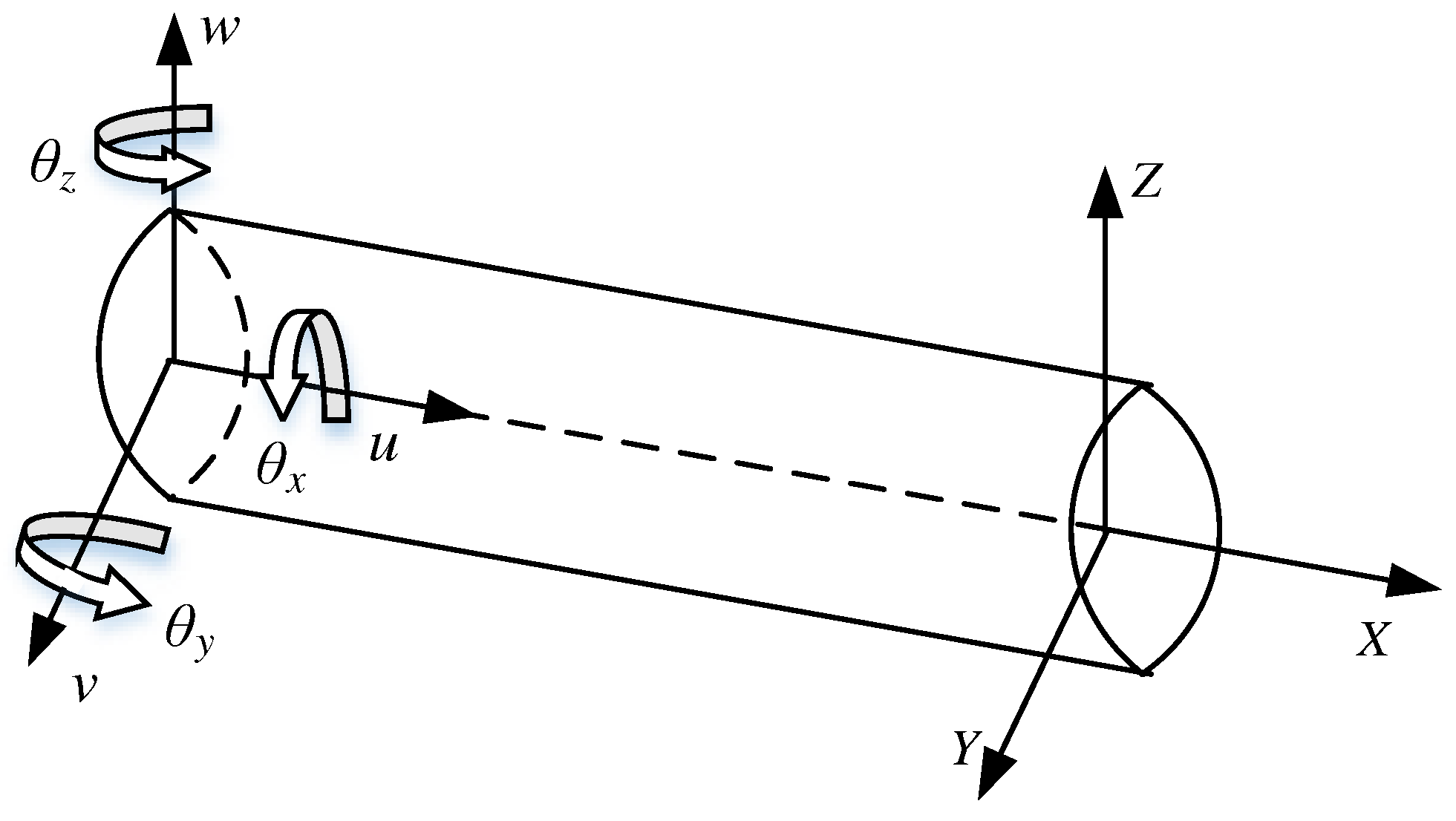
As shown in Figure 2, taking the Timoshenko beam as an example, the deformation of this neutral axis is determined by the displacements u,v,x along each axis and the rotation angles θx, θy, θz of each axis, the strain values are obtained from the strain sensors affixed to the surface of the structure, and the nodal DOF are determined by Eq.s (4)-(9) and expressed as Eq. (10)
u = [ u , v , w , θ x , θ y , θ z ] T
where u,v,w,θxyz are also called the kinematic variables of the nodal DOF u. When the nodal DOF u(x) are determined, the shape function H(x) is obtained by interpolation of the nodal DOF, and the displacement d of the final reconstruction is determined by the shape function and the nodal DOF, as in Eq. (11).
d = { d x d y d z } = [ 1 0 0 0 z - y 0 1 1 - z 0 0 0 0 1 y 0 0 ] [ u ( x ) v ( x ) w ( x ) θ x ( x ) θ y ( x ) θ z ( x ) ] = H ( x ) u ( x )

3. Coarse and Fine Two-Stage Calibration Method

3.1. Coarse Calibration

When the layout position of the strain sensor is determined, human installation factors will cause the sensor pasting position to offset, thus affecting the accuracy of the displacement-strain transformation matrix Tk associated with the sensor position in Eq. (9), resulting in an error ΔTk between the theoretical displacement-strain transformation matrix Tk and the actual displacement-strain transformation matrix Tk' after the sensor is installed, as shown in Eq. (12).
T k ' = T k + Δ T k
To reduce the effect of sensor position offset on the reconstructed displacement accuracy, an error compensation method based on a single-objective particle swarm algorithm is proposed for the displacement-strain transformation matrix.
The Root Mean Square Error (RMSE) is defined as
R M S E = 1 n m = 1 n ( d i s p i u - d i s p i v ( P ' ) )
The Relative Root Mean Square Error (RRMSE) is defined as
R R M S E = R M S E m a x ( d i s p u ) × 100 %
where n denotes the number of position sensors (check points). P' denotes the actual installation positions of the 6 strain sensors (i=1,2,. .6), which consists of the actual overall sensor layout position when the strain sensor installation position is offset.
After the installation of the strain sensor, the strain value during the deformation of the structural body is measured and the theoretical displacement value d i s p i v is obtained based on the iFEM reconstruction. d i s p i u denotes the actual measured displacement at check points.
The sensor position optimization model based on iFEM is shown in Eq. (15),
M i n m i z e   I n d e x ( P ' ) = [ R R M S E ( P ' ) ] P ' = ( P 1 ' , P 2 ' , P 3 ' , P 4 ' , P 5 ' , P 6 ' )
where the exponent (P') denotes the objective function of optimization. And in this paper, the number of sensors required for the displacement field reconstructed is six [22].
Since the specific offset position cannot be obtained after installation, According to the actual situation, the optimization range can be set around the theoretical installation position of the sensor extracted in the simulation software ANSYS. the optimized sensor position parameter (xi*,θi*,βi*) can be obtained based on the single-objective particle swarm algorithm. and the modified displacement-strain matrix T k * can be obtained by substituting the parameter (xi*,θi*,βi*) into Eq.s (6-9), improving the reconstruction accuracy of the displacement field.
Particle swarm optimization (PSO) is an evolutionary computational technique. All particles in the swarm adjust their velocity and position according to the current individual extreme value they find and the current global optimal solution shared by the whole swarm.
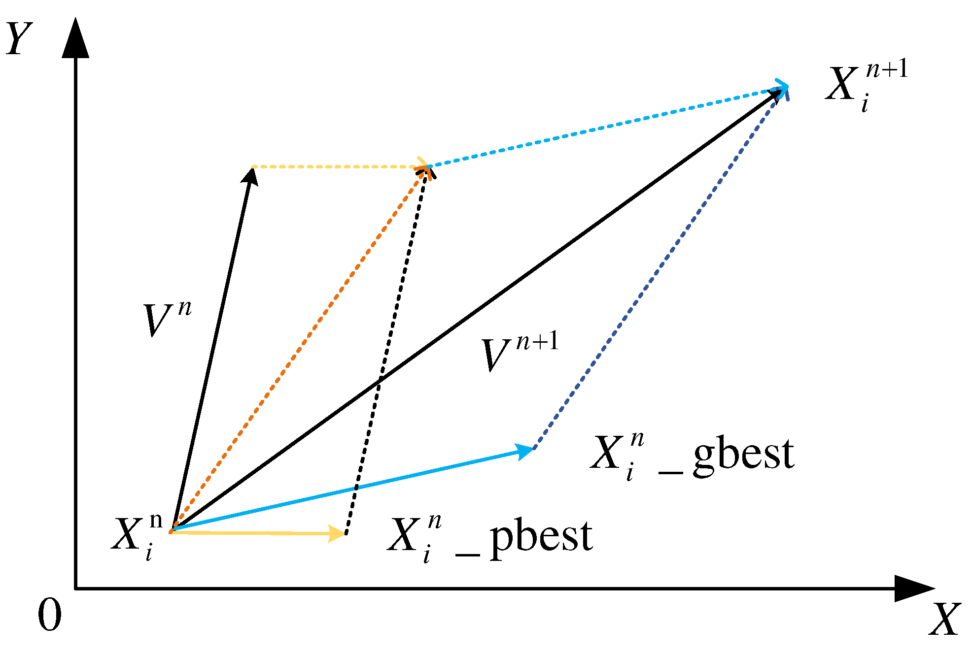
The basic idea of PSO is to search for optimal solutions to optimization problems through collaboration and information sharing among individuals in a population. As shown in Eq. (16)(17).
V n + 1 = V n × w + c 1 × r a n d _ f 1 × ( X i n _ p b e s t - X i n ) + c 2 × r a n d _ f 2 × ( X i n _ g b e s t - X i n )
X i n + 1 = X i n + V n + 1
where the inertia factor w is a value between 0 and 1. As the number of iterations increases, X i n   denotes each position parameter of each particle, which in this paper means the position of the sensor.c1 and c2 denote acceleration factors, rand_f1、rand_f2 are random values between 0 and 1, and X i n _ p b e s t is denoted as individual optimum, indicating the optimal position of particle Xi in the previous generation during the iterative process, and X m n _ g b e s t is denoted as population optimum, indicating the best position explored by all individuals in the population.
The fitness function f(Xi) of PSO is obtained by solving the optimization model in Eq. (15). The iterative process is shown in Eq. (16) (17), and the particle moves from Xi to X i n with the updated velocity Vn as shown in Figure 3.
The steps for solving the optimization model (15) based on the single-objective particle swarm algorithm are shown below.
Step 1: Initialize the initial position X0 and initial velocity V0 of the particle swarm algorithm, setting them within the installation error of the sensor. The number of population size is set to N=80 and the maximum number of iterations is nmax=100.
Step 2: In each generation of evolution, the value of the fitness function f( X i 1 _ p b e s t ) is calculated for each particle, compare whether the current adaptation value of each particle is better than the historical local optimum, i.e., f( X i 1 ) > f( X i 0 _ p b e s t ), and take the current particle adaptation value f( X i 1 )as the local optimum of the particle, and then its current position is taken as the optimal position of the particle. And the current adaptation value of each particle is compared with the adaptation value f( X m n _ g b e s t ) corresponding to the global best position X m n _ g b e s t , if the current adaptation value is higher, the global best position will be updated with the current particle position.
Step 3: the algorithm iterates to the maximum number of iterations, n=nmax, the algorithm terminates.
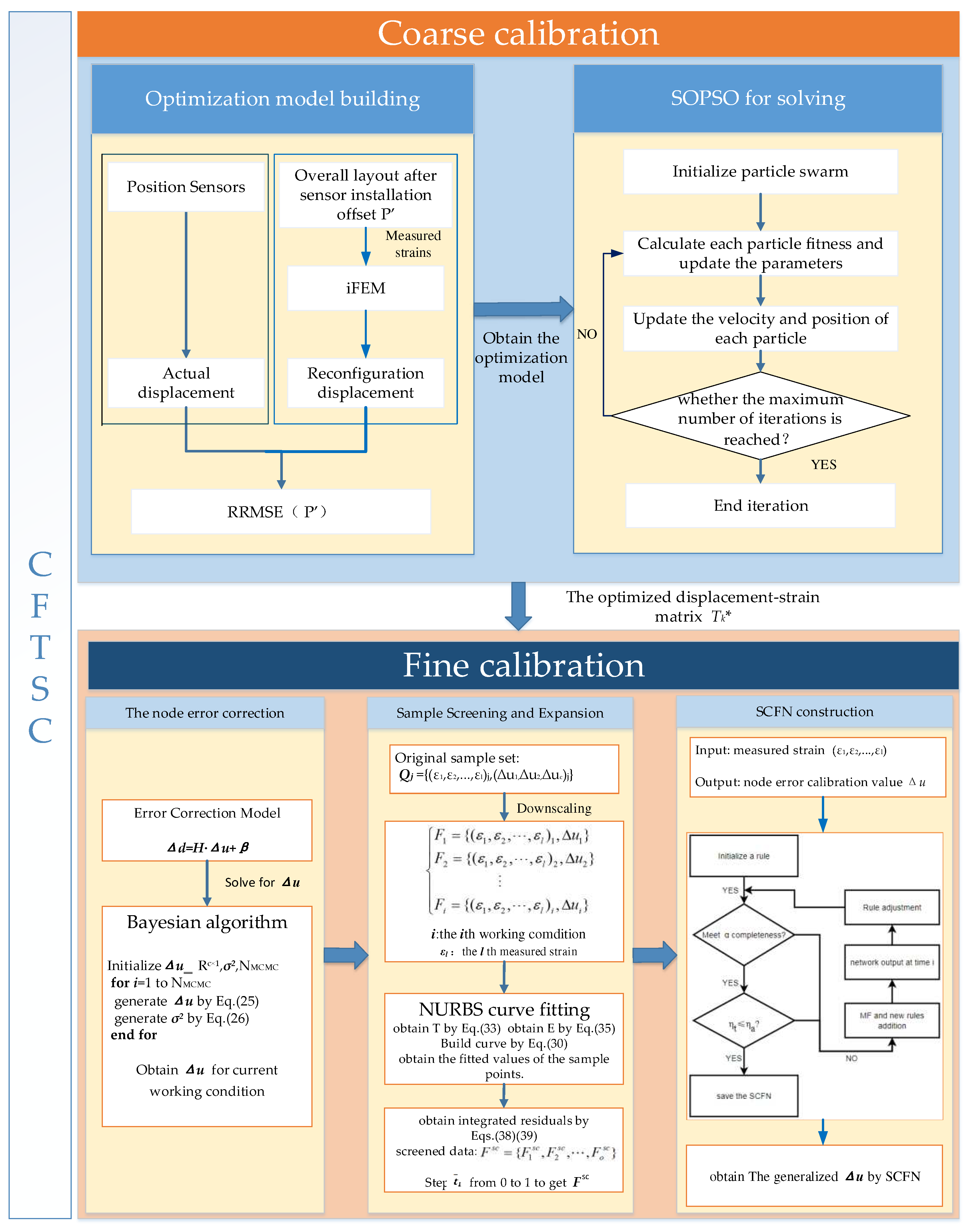
In summary, we call this method of displacement error calibration as coarse calibration. The coarse calibration process is shown in Figure 5. And on the basis of the coarse calibration method. The fine calibration is performed in 3.2 to further improve the reconstruction accuracy of the deformation field.

3.2. Fine Calibration

3.2.1. The Nodal Degrees of Freedom Error Correction

For the errors that still exist between the displacements reconstructed based on the iFEM and the actual displacements after the coarse calibration, the displacement-nodal degree of freedom error correction model is further proposed. As shown in Eq. (18), the theoretical displacement of the inverse finite element reconstruction is denoted as d i t , and the actual displacement is denoted as d i a
d i a = d i t + Δ d i
where i=1,... ,n denotes the ordinal number of observation points and Δdi denotes the reconstruction error. Displacement at any position in the structure can be obtained from the shape function H(x) and the discrete nodal during the reconfiguration displacement. As a result, correcting the reconstruction error in the nodal DOF enables calibration of the entire displacement.
The relationship between displacement error and nodal DOF error can be expressed as Eq. (19).
Δ d i = [ Δ d i x Δ d i y Δ d i z ] = G × N i × Δ u
where the number of nodal DOF is c. The displacement field error Δdi of the inverse finite element reconstruction is derived by Eq. (19) to the nodal DOF error Δuj(j= 1, ... , c), then the displacement-nodal DOF model can be expressed as Eq. (20)
Δ d z = H Δ u + β
where Δdz=[Δ d 1 z , Δ d 2 z , ... ,Δ d n z ]T, H=[H1.H2,... ,Hn], β is denoted as the residuals after displacement error correction and obeys Gaussian distribution. i.e., β ~ N ( 0 , σ 2 ) , and H i = [ H i 1 , H i 2 , , H i c ] is the row vector of G*Ni for Δdz.It follows that Δdx and Δdy can also be expressed analogously by Eq. (20).
The matrix H in Eq. (20) is the ill-conditioned matrix. The actual measured strain value of the sensor receives interference from random noise, which makes the estimated value Δu having error with the actual value, the error is reduced by Bayesian regularization algorithm using prior information. From Bayesian theory, pΔu,σ2|Δdx)is used to represent the joint posterior distribution of the unknown parameters, as defined as shown in Eq. (21):
p ( Δ u , σ 2 | Δ d x ) p ( Δ d x | Δ u , σ 2 ) p ( Δ u , σ 2 )
where p(Δu,σ2) denotes the joint prior distribution, rewriting Eq. (21) into multiplicative form. where it is assumed that the residuals are independently Gaussian distributed, i.e., β = [ d x H · u ] N ~ ( 0 , σ 2 ) , the non-informative prior of σ2 is taken into account, i.e., p ( σ 2 ) 1 / σ 2 . Assuming that the prior distribution of Δu is Gaussian, i.e., p ( u ) = N ( 0 , τ 2 ) , the posterior distribution in logarithmic form ln p = ( u , σ 2 | d x ) is represented
l n p ( Δ u , σ 2 | Δ d z ) - i = 1 n [ Δ d i z - H i Δ u ] 2 - λ j = 1 c Δ u j 2
where λ = σ 2 τ 2 ,The conditional posterior distribution of Δu in Eq. (23) is calculated using the conjugate distribution method as N(Δuj, s j 2 ) .
Δ u j = ( i = 1 n x i j 2 + λ ) - 1 i = 1 n x i j ( Δ d i z - j = 1 , j j c x i j Δ u j ) s j 2 = ( i = 1 n x i j 2 ) - 1 σ 2 + τ 2
For σ2, the conditional posterior distribution is the inverse chi-square distribution, expressed as
σ 2 ~ 1 χ 2 i = 1 n ( Δ d i z - j = 1 c x i j Δ u j ) 2
Therefore, Markov Chain Monte Carlo samples are produced from the posterior pΔu,σ2|Δdx)via a Gibbs sampler for calibration amounts Δu ,the steps are as follows: (1) initialize Δu and σ2; (2) perform Gibbs sampling on Δu in Eq. (23); (3)The inverse chi-square distribution from Eq. (24) is selected σ2. The specific process details are shown in Figure 4.
The calibration values of each kinematic variable in the nodal DOF error are derived from the Bayesian regularization algorithm and are combined with the actual measured strain values to form the sample data, defining in Eq. (25).
Q j = { ( ε 1 , ε 2 , ... , ε L ) j , ( Δ u 1 Δ u 2 , ... , Δ u m ) j }
where Qj denotes the j th (j=1,2, ... , h) sample data under working conditions, ε l denotes the l th (l=1,2,... ,L) strain value measured by the sensor. ∆ui (i=1,2,...,m) denotes the error calibration value of the kinematic variable in the nodal DOF error.

3.2.2. Training Data Filtering and Sample Size Expansion

The error correction method has limitations: the nodal DOF errors can only be calibrated under specific working conditions. Therefore, in order to obtain the error calibration between strain values and nodal DOF under arbitrary working conditions, a self-constructed fuzzy network is used for calibration. The selection of appropriate training data affects the training effect of self-constructed fuzzy networks, and this paper employed the residual analysis to screen the sample data. In addition, the training effect of the self-constructed fuzzy network is also related to the number of training samples, so the number of training samples should be expanded before entering the training network.
The residual is the difference between the actual observed value and the fitted value of the sample. The reliability and reasonableness of the data is analyzed using the residual, defined as follows.
e = y - y ^
where y represents the actual observed value, y ^ represents the fitted value, and e represents the residual.
In this paper, considering that high-dimensional data can cause excessive computation, and the screening of sample data requires residual analysis for each kinematic variable in the calibration values of DOF to ensure the reasonableness of screening training data.
The new sample point is obtained by downscaling the original sample data Qj in Eq. (25)
{ F 1 = { ( ε 1 , ε 2 , , ε l ) 1 , Δ u 1 } F 2 = { ( ε 1 , ε 2 , , ε l ) 2 , Δ u 2 } F m = { ( ε 1 , ε 2 , , ε L ) m , Δ u m }
Decompose each sample point is decomposed into Fi (i=1,2,... ,m) of the form, where each vector Fi consists of L measured strain values ε L and 1 kinematic variable of nodal DOF error,and denote the kinematic variables as Δui (i=1,2,... ,m).
The sample fit values were obtained before the sample data were screened based on the magnitude of the residuals. In this paper,
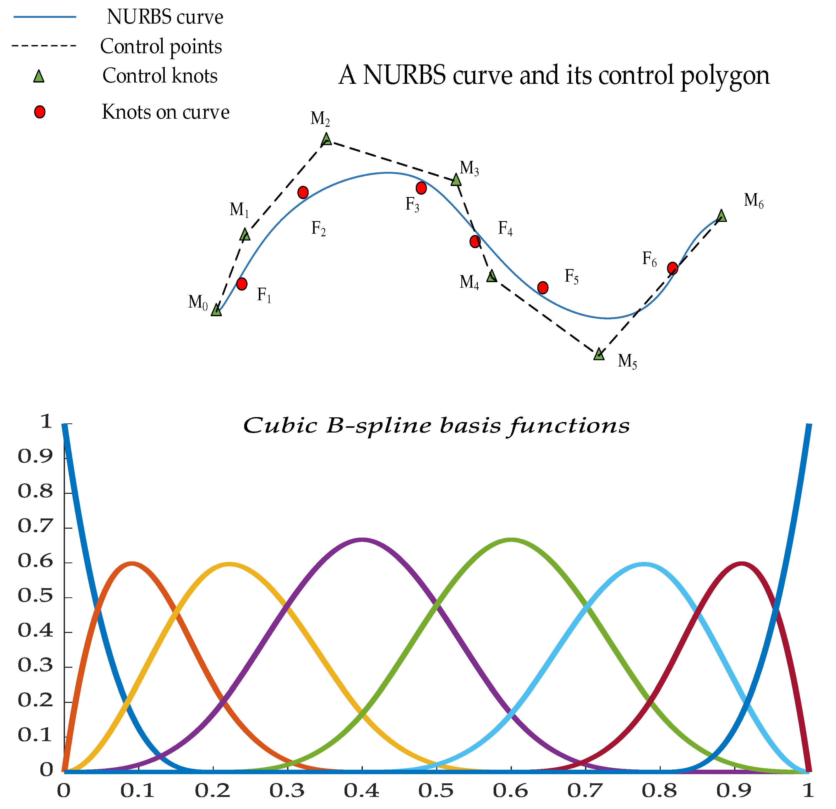
the Non Uniform Rational B-spline (NURBS) curve fitting method is used to fit the data Fi, as shown in Figure 4.
The NURBS curve of order c can be expressed as a segmented rational polynomial vector function, the mathematical definition is as follows.
p ( t ) = i = 0 h k i M i E i , c ( t ) i = 0 h k i E i , c ( t )
where ki (i=0,1,... ,h) denote the weight factors, respectively, associated with the control vertex Mi (i=0,1,...,h),due to the lack of expert experience, the weighting constants ki=1 (i=0,1,... ,h). Ei,c(t) denotes the c-th order B-spline basis function, which is a non-decreasing sequence of parameter. T=[t0,t1,…,th+c+1] is the nodal vector and determined by the c-th order segmented polynomial.
The basis function can be recursively expressed by.
E i , 0 ( t ) = { 1 , t i t t i + 1 0 , o t h e r w i s e E i , c ( t ) = t - t i t i + c - t i E i , c - 1 ( t ) + t i + c + 1 - t t i + c + 1 - t i + 1 E i + 1 , c - 1 ( t )
The parameterization of the data points reflects the nature of the curve constructed with the data points. Based on the nodal vector of basis functions and control points to construct the NURBS-fitted curves. A centripetal parameterization method is applied to the sample data as shown in Eq. (30).
{ t ¯ 0 = 0 t ¯ i = t ¯ i - 1 + | F i - F i - 1 | 1 2 i = 1 h | F i - F i - 1 | 1 2 t ¯ h = 1 ( i = 1 , 2 , , h - 1 )
As required by the definition domain of the non-closed curve, multiple knot with repetition degree c+1 are taken at the two endpoints of the definition domain. According to the distribution of the sample and the method of centripetal parameterization, the non-uniform vector method is used for the construction, shown in Eq. (31).
{ t 0 = t 1 = = t c = 0 t j + c = 1 c i = j j + c - 1 t ¯ i ( j = 1 , 2 , , h - c ) t h + 1 = t h + 2 = = t h + c + 1 = 1
The c-th order NURBS curve is constructed by m+1 sampling points Fi (i=0,1,... ,m). The approximation function is obtained by using the least squares method to approximate the parameter sequence t i ¯ (i=0,1,... ,m), shown in Eq. (32).
δ ( p , t ¯ ) = i = 1 m F i - p ( t i ¯ ) 2
where the control points are set to A0=F0, Am=Fh,then Si=Fi-F0E0,c( t ¯ i )-FhEp,c( t ¯ i ). and the partial derivatives of the control points in Eq. (32) are equal to 0.
The matrix form is expressed as.
M ( E T E ) = S
where the E matrix is a matrix with h-1 rows and m-1 columns and ET is the transpose matrix of E. The E, S, and M matrices are shown in Eq. (34).
E = [ E 1 , c ( t 1 ¯ ) E 2 , c ( t 1 ¯ ) E h - 1 , c ( t 1 ¯ ) E 1 , c ( t 2 ¯ ) E 2 , c ( t 2 ¯ ) E h - 1 , c ( t 2 ¯ ) E 1 , c ( t m - 1 ¯ ) E 2 , c ( t m - 1 ¯ ) E h - 1 , c ( t m - 1 ¯ ) ] S = [ E 1 , c ( t 1 ¯ ) E 2 , c ( t 1 ¯ ) E h - 1 , c ( t 1 ¯ ) E 1 , c ( t 2 ¯ ) E 2 , c ( t 2 ¯ ) E h - 1 , c ( t 2 ¯ ) E 1 , c ( t m - 1 ¯ ) E 2 , c ( t m - 1 ¯ ) E h - 1 , c ( t m - 1 ¯ ) ] T [ s 1 s 2 s m - 1 ] M = [ M 1 M 2 M h - 1 ]
The specific steps to obtain the sample fit values using NURBS curve fitting are as follows:
(1) the data are parameterized by Eq. (29) to obtain t ¯ i (i=1,2,... ,m). and the basis function Ei, c(t).
(2) After obtaining t ¯ i , the nodal vector T is obtained by Eq. (30).
(3) The control point Mi (i=1,2,... ,h) is obtained according to Eq. (33).
(4) The constructed NURBS fitting curve is then derived from Eq. (28).
(5) When the NURBS fitted curve is obtained, the values of the sample data parameters are substituted into the curve Eq. of Eq. (28), and then the values on the fitted curve corresponding to the original sample data can be obtained.
Similarly, the fitted data F ^ i (i=1,2,... ,m) for the rest of the samples under a working condition can be obtained as shown below.
{ F ^ 1 = { ( ε ^ 1 , ε ^ 2 , , ε ^ L ) 1 , Δ u ^ 1 } F ^ 2 = { ( ε ^ 1 , ε ^ 2 , , ε ^ L ) 2 , Δ u ^ 2 } F ^ m = { ( ε ^ 1 , ε ^ 2 , , ε ^ L ) m , Δ u ^ m }
When screening training data using residual analysis, the error in the kinematic variables Δui (i=1,2,...,m) varies considerably in order of magnitude due to the actual situation, which affects the residual analysis. The transformation matrix H in Eq. (2) is related to the observed coordinates of the position sensor (check point) and other factors, and the order of magnitude of each column of the transformation matrix H varies greatly. According to Eq. (19), Δdi for the same working conditions is generally under the same order of magnitude, so it leads to kinematic variable errors Δui (i=1,2,...,m) obtained from the solution of different orders of magnitude.
According to the analysis described above, the main factor affecting the magnitude of the kinematic variable error is the column vector of transformation matrix H. Therefore, the weighting constants are calculated as shown in Eq. (36).
a i = 1 v k = 1 v H k i
where ai (i=1, 2, ... ,m) denotes the weighting constants corresponding to the mth kinematic variable error, and Hki denotes the k-th row and i-th column of the transformation matrix.
When the position of the position sensor is fixed, the matrix H is fixed under any working condition, so the weighting constants corresponding to the kinematic variable error are also unchanged. At this time, The integrated residual value et of sample under one working condition can be obtained from the Euclidean distance, which is calculated as shown in Eq. (37).
e t = i = 1 m ( a i ( Δ u i - Δ u ^ i ) ) 2
In summary, the integrated residuals of the samples e j t (j=1,2,....,h) under the remaining working conditions can be obtained.
The screened training data consists of three parts: boundary samples, representative samples and normal samples after equidistant sampling. the boundary samples are the sample points where the structure is in the minimum and maximum load states in the experiment. After extensive experiments and summaries, it is concluded the normal sample points in the remaining sample points are all the values with small fluctuation range of residuals, And the residual values of representative sample points are more than twice the fluctuation range of the residual values of normal sample points.
The specific steps of the screening training data method are: (1) The NURBS curve fitting method is adopted to obtain the corresponding fitting data of sample points. (2) Subtracting the corresponding fitting data from the sample data to obtain the residual values of each sample point under different working conditions. (3) Selecting the boundary samples, representative samples, and normal samples obtained by equidistant sampling as the training samples for constructing the self-constructed fuzzy neural network.The training sample set Fsc are screened from all samples Qj is denoted as:
F s c = { F 1 s c , F 2 s c , , F o s c } o j
Expanding the number of screened training samples F o s c through the NURBS curve fitting method. After obtaining the fitting curve, a specific step is taken to extend the sample quantity by substituting values of t ¯ i ranging from 0 to 1 into Eq. (28). Then, self-constructed fuzzy network is trained based on the extended samples.

3.2.3. Self-Constructed Fuzzy Network Calibration

Due to the nonlinearity and coupling relationship between the strain values in the sample data and the nodal DOF calibration values, it is difficult to establish a mathematical model. However, SCFN can effectively solve this nonlinearity problem. After screening all samples for suitable training samples and extending them, the SCFN is trained based on the extended samples. A strain-nodal DOF calibration model is established. The SCFN enhances the generalization ability of the strain-nodal DOF calibration value and improves the accuracy of the reconstructed displacement by calibrating the nodal DOF. SCFN is divided into two steps [31]: (1) Adding the affiliation function and generating the corresponding fuzzy rules. (2) Adaptively adjust the results of the fuzzy rules.
In this paper, because the triangular affiliation function has a simple structure, it is convenient to calculate the membership degree and efficient. Thus, SCFN chooses the triangular membership function and the 0th order T-S fuzzy model, which is represented by the fuzzy rule set as follows.
S n : i f ε 1 i s R 1 n a n d ε 2 i s R 2 n a n d ε K i s R K n t h e n p ^ n = w n
where Sn (n=1,2,...,N)denotes the nth fuzzy rule, ε k (k=1,2,... , K) is denoted as the input strain value, and R n k denotes the membership degree corresponding to ε k in the nth rule. p ^ n denotes the output of the nth fuzzy rule and w n is the value corresponding to its fuzzy rule output.
The system output of SCFN ̂ p ^ represents the nodal DOF error, and when a certain input activates m rules (n≥m), the system output is derived from the p ^ n of these m outputs by weighted averaging, as shown in Eq. (33).
Y ^ = n = 1 m q n p ^ n n = 1 m q n = q 1 p ^ 1 + q 2 p ^ 2 + + q m p ^ m q 1 + q 2 + + q m
The q n in Eq. (40) denotes the weighting constants of the rule, and the weighting constants are calculated by taking the smallest method, as shown in Eq. (41).
q n = R 1 n R 2 n L R K n = k = 1 K R k n ( ε k )
The SCFN is initialized with one rule, and the membership functions and rule number are added or removed based on the error and completeness criteria. When the number of training samples is k+1, the error standard of SCFN is represented by root mean square error ηt, and the formula is shown below.
U ^ ( c ) η t = c = 1 k ( U ^ ( c ) - U ( c ) ) 2 k
where denotes the actual output, U(c) denotes the desired output, ηa is denoted as a predetermined error threshold, and if ηta, it means that the system error does not meet the requirements and the membership function needs to be increased.
In SCFN, each input value at least corresponds to one membership function, if its membership degree R k n is greater than the completeness threshold α, the completeness of the membership function meets the requirements, if R k n is less than α, it is necessary to increase the membership function and fuzzy rules. The completeness threshold is generally set to 0.5.
After adding the membership function and fuzzy rule, the fuzzy rule also needs to be adaptive adjustment to make it closer to the output value. The specific expression for adjusting the nth rule of the fuzzy controller at the ith moment is as follows.
a n ( i ) = a n ( i - 1 ) + V φ n ( i - 1 ) ( U ( k - 1 ) - U ^ ( k ) )
where an(i) denotes the rule adjustment result at moment i, V is used to adjust the adaptive speed during rule adjustment, φn(i-1) denotes the weighting constants of the nth rule at moment i-1, P(i-1) denotes the desired output of the nth rule at moment i-1, and (i) is the current system output.
p ^ Each rule is added and adaptively adjusted according to the standard correspondence, and then used to train the SCFN. when ηtηa, the training is stopped to jump out of the iteration and generate the fuzzy network, and the trained fuzzy rules are saved to obtain the calibrated nodal freedom results.
Summarize the above, The method flow framework for CFTSC method is shown in Figure 5.
Figure 5. Flow framework of CFTSC method.
Preprints 74010 g005

4. Experimental Research

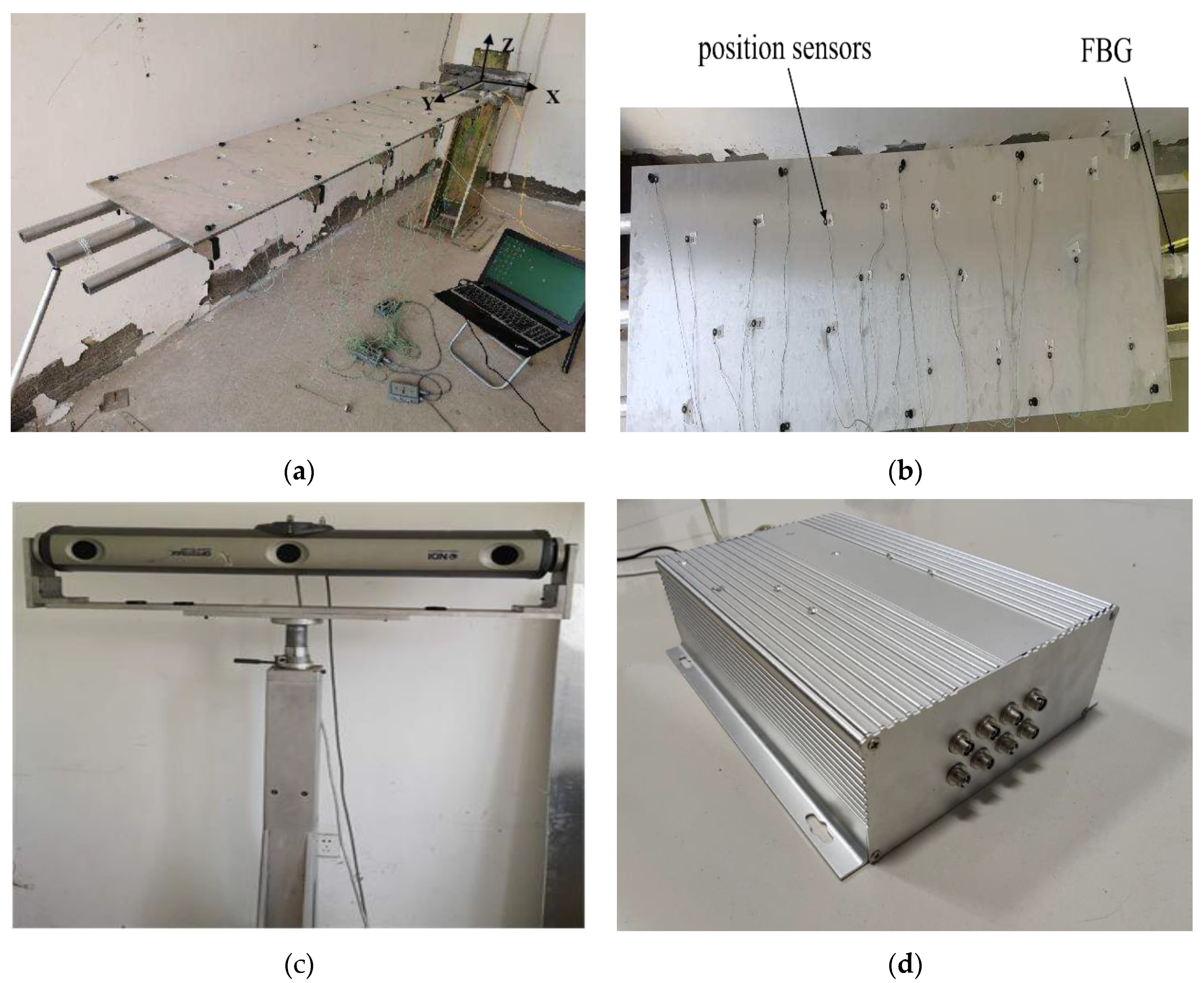
In order to verify the effectiveness of the CFTSC method proposed in this paper, the wing-integrated conformal antennas structure is considered as experimental object. Experimental subjects is a plate and beam integrated structure, and the structure body consists of three beams and an aluminum plate. The beams and plate are connected by six steel bars and three beams are connected with fixed ends. Each beam is made of aluminum alloy and has a length of 2000 mm. The beam located in the middle of the three beams has an outer radius of 40 mm and an inner radius of 32 mm. The remaining two beams located on the sides have an outer radius of 30 mm and an inner radius of 24 mm. The specification of the plate in the structure is an aluminum plate with a length of 1120 mm, a width of 400 for mm, and a thickness of 8 mm, placed and attached above the three beams with the plate 500 mm from the fixed end, as shown in Figure 6(a).
The Fiber Bragg Grating (FBG) demodulator is used to read the wavelength information collected by the six FBG strain sensors installed on the main beam of the structure during the deformation process, The strain values during the structural deformation are then calculated by the host computer. The specific information of the sensor installation is shown in Table 1. xp indicates the relative position of the sensor on the beam, and (θ, β) respectively indicate the circumferential angle on the circular section and the angle with the X-axis when the sensor is installed.
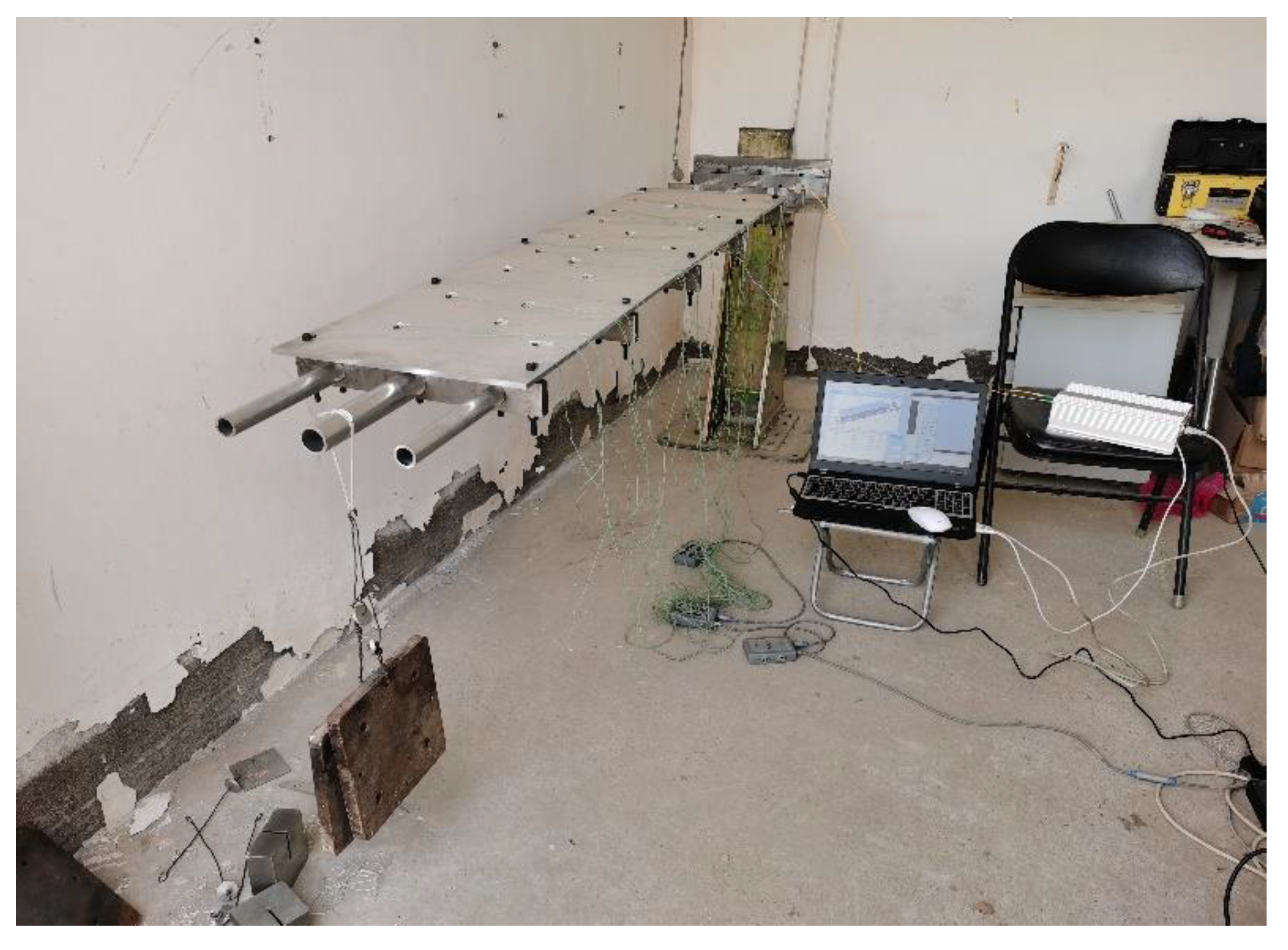
In Figure 6(b), the information of the position sensors (marked points) installed on the surface of the aluminum plate is collected by the 3D optical measuring device NDI (Northern Digital incorporated) with a measurement accuracy of about 0.1 mm. the position sensors can obtain the deformation of the structure dynamically in real time obtain the three-dimensional coordinates in the X, Y, and Z directions. As shown in Figure. 6(a), the coordinate system in X, Y, and Z directions is established at the fixed end of the structure. From Table 2, The position information of the 10 position sensors installed after establishing the coordinate system can be obtained. In this experiment, the strain values collected by the FBG sensor through the demodulator system and the position information collected by the position sensor of NDI are performed simultaneously, and Figure 7 shows the overall system of the experiment.
Relative to the fixed end, the load is added to the main beam at the other end of the structure (free end), as shown in Figure 7, the magnitude of the static load under all working conditions is shown in Table 3. The CFTSC method calculates the displacement under various working conditions based on the strain values collected according to the concentrated load forces listed in Table 3.
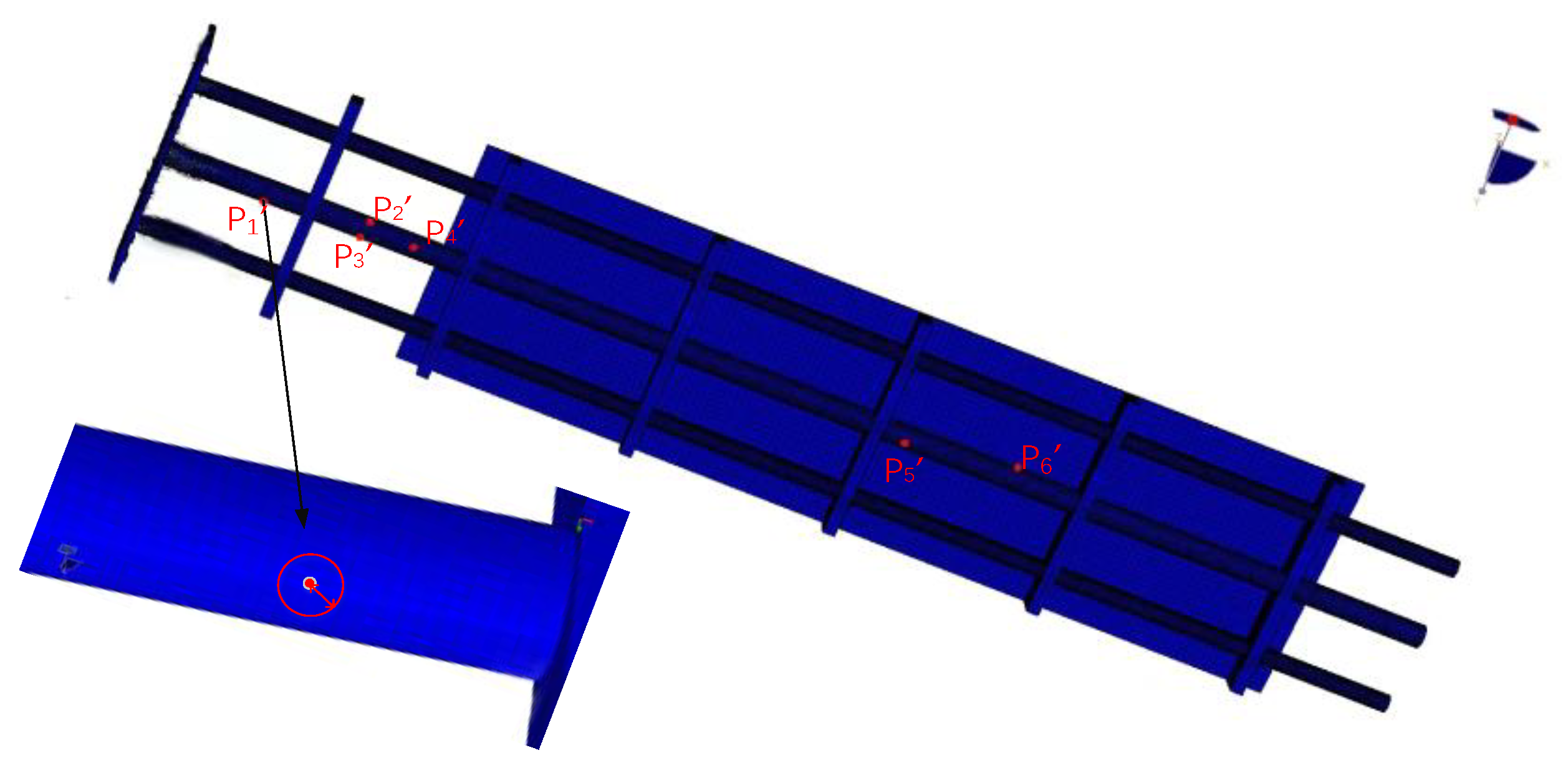
T T The experiments of coarse calibration were first performed to verify the calibration effect. The information read by the FBG demodulator system is obtained, and the theoretical displacement values of the structure at the 10 position sensors are reconstructed based on the iFEM, And the actual deformation is measured by NDI, the index is assessed by Eq. (15). When the strain sensors are manually installed according to the layout determined in the simulation software ANSYS, the error of the position offset between the actual attachment position and the theoretical position in ANSYS is within 1 cm. Therefore, the particle swarm optimization range of each strain sensor position information is set to be within 1 cm around the theoretical position in ANSYS and within ±30° of angle. Taking strain sensor P1’ as an example, as shown in the Figure 8. The optimization range for the remaining sensors is the same.
The optimized sensor position parameters are obtained based on the single-objective particle swarm optimization algorithm, and then the optimized displacement-strain matrix is derived from Eq. (6) to Eq. (9) based on the optimized sensor position parameters. In order to test the effect of the coarse calibration method on the reconfiguration accuracy effect, indicators for estimating the calibration accuracy are proposed, which are defined as.
R M S E = i = 1 N ( d i s p n ( i ) - d i s p c ( i ) ) 2 N
where the superscript ‘n’ indicates the actual displacement measured by NDI, ‘c’ indicates the calibrated displacement by the coarse calibration method, and ‘m’ indicates the reconstructed displacement by the iFEM. N indicates the number of position sensors.
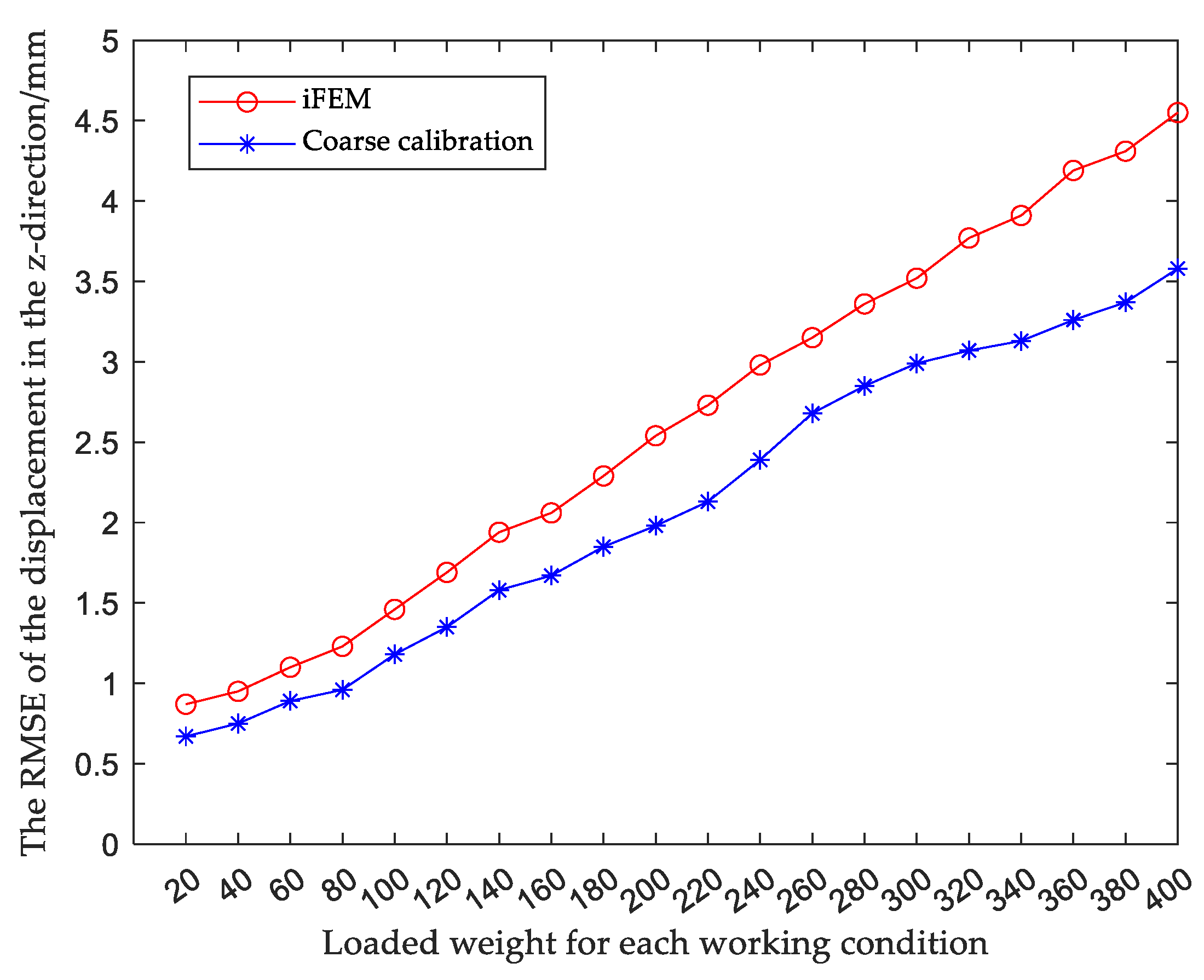
when the structure is in a certain working condition, the relative root mean square error (RMSE) in the z-direction of the main deformation direction after coarse calibration is obtained from Eq. (44), similarly, the RMSE in the rest of the working conditions can be obtained. and compared with the RMSE obtained by reconstructing the displacement using the iFEM, as shown in Figure 9, and the specific data are shown in Table 4.
The results show that compared with traditional iFEM, the calibration accuracy of the observed values for each working condition is improved by using the coarse calibration method. Next, fine calibration is performed on the basis of the coarse calibration to further improve the displacement reconstruction accuracy.
On the basis of the modified T k * matrix obtained by coarse calibration, the displacement field is reconstructed by the iFEM. The reconstructed displacements are compared with the actual displacements obtained from the 3D optical measuring instrument NDI, the reconstructed displacement error Δdi is obtained from Eq. (18), then the nodal DOF error Δu is obtained from Eq. (20).
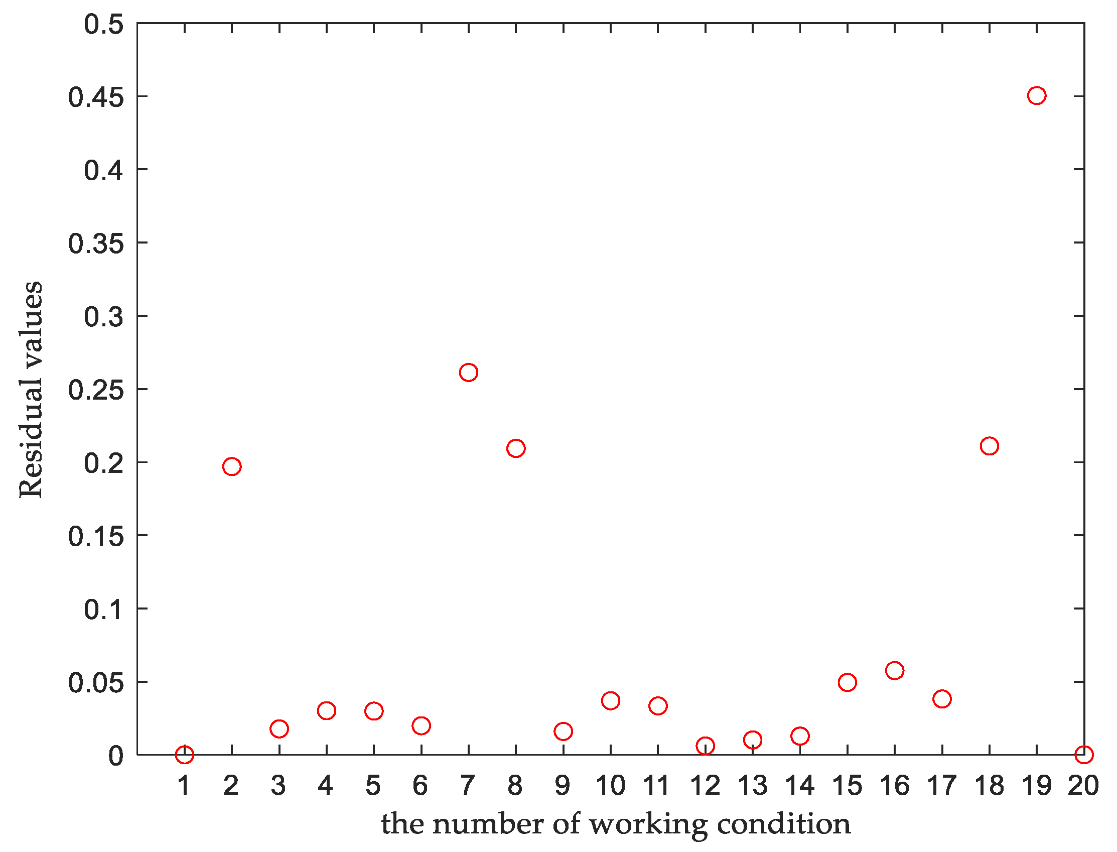
After the original sample data were downscaled, the fitted values of each kinematic variable were obtained by NURBS fitting, the corresponding weighting constants of each kinematic variable are calculated by Eq. (36), and the integrated residuals of kinematic variable under each working condition are obtained by Eq. (37), the residual plots for each working condition are shown in Figure 10. The integrated residuals of these 20 sets of working conditions were analyzed, and the residual values of most samples fluctuated in the range of 0-0.1, which are set as normal samples, samples with residual values 2 times or more than the normal samples are set as representative samples. The boundary samples, representative samples and equidistantly sampled normal samples were used together as training samples, and the rest as test samples. 13 sets of training data and 7 sets of test data were selected, as shown in Table 6 and Table 7.
The NURBS curves with 20 control points are fitted with these 13 sets of training data, and the fitted curves are sampled at equal intervals and expanded to generate 200 sets of data from the 13 sets of sample data. The expanded data are then used to construct a self-constructed fuzzy network with the input value of strain, and the calibrated nodal DOF is output through the trained self-constructed fuzzy network. Finally, the calibrated displacement values are obtained according to Eq. (2) based on the calibrated nodal DOF and the shape function H(x). In order to verify the verification accuracy of the CFTSC, the calibration accuracy index are shown.
Error = | d i s p n d i s p c f |
MER = MAX | d i s p n ( i ) d i s p c f ( i ) |
RMSE = i = 1 N ( d i s p n ( i ) d i s p c f ( i ) ) 2 N
where the superscript 'cf' indicates the CFTSC method. MR denotes the maximum displacement of the structure. The error is indicated by the absolute error, and MER indicates the maximum absolute error. When the load is at the maximum load state (400N), the maximum displacement value in the z-direction of the main deformation direction is 158.83mm.
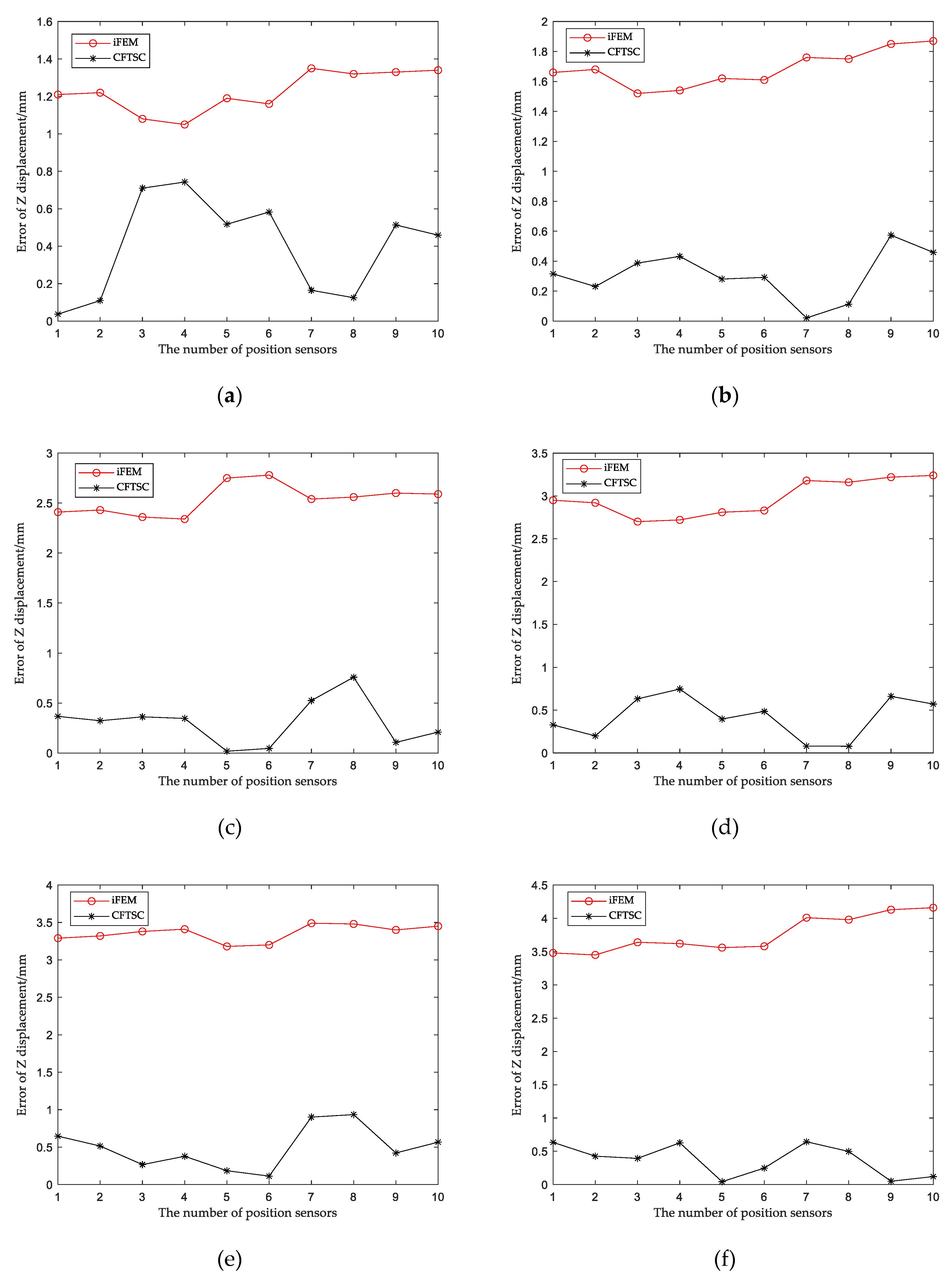
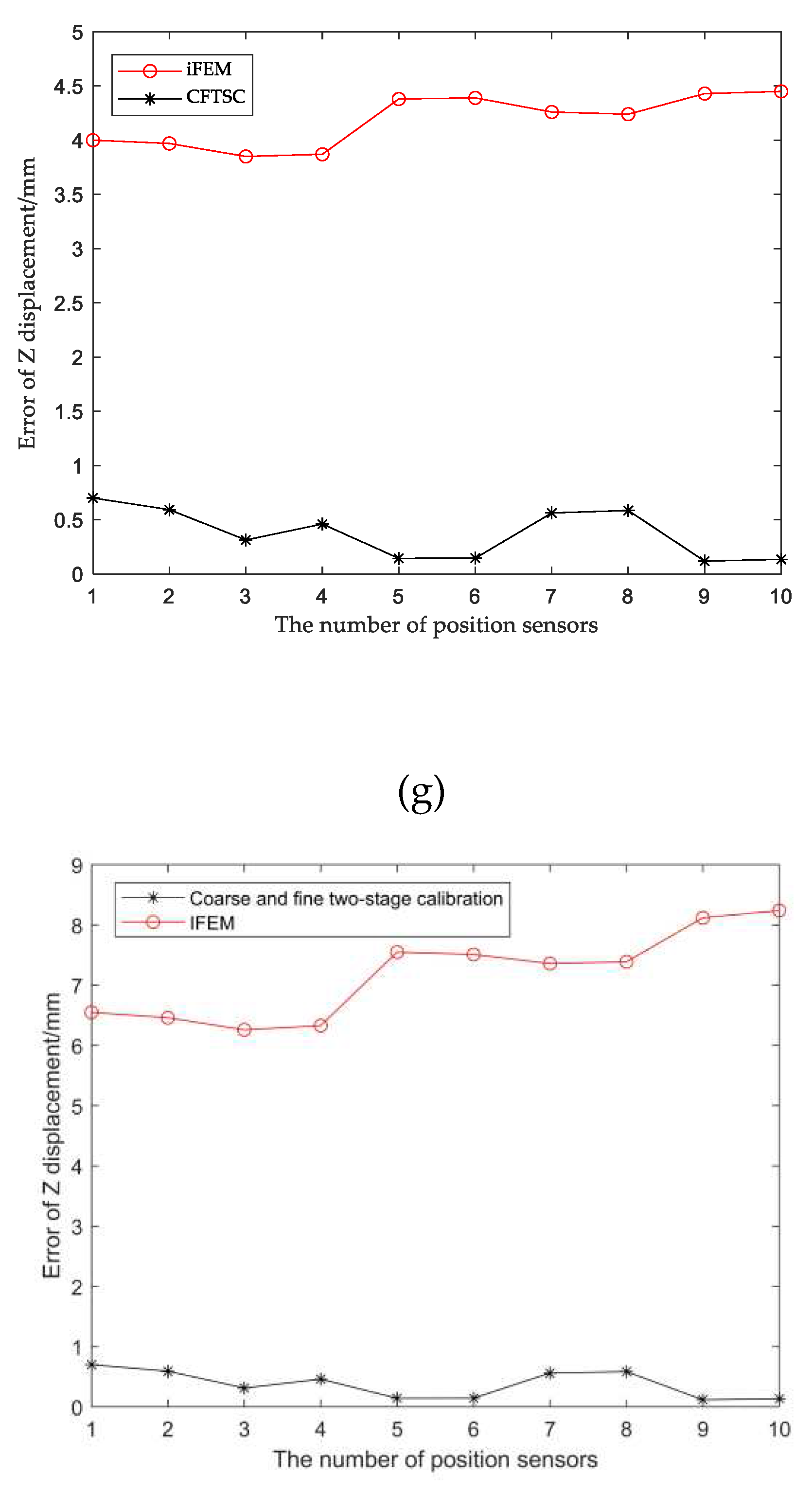
The calibration effect of CFTSC was tested with 7 sets of screened test data, and the calibration results of each set of test data are shown in Figure 11 (a)-(g). The experimental results show that the displacement accuracy of the 7 sets of test data is greatly improved compared with the traditional iFEM.
The reconstruction displacement error in the z-direction at the check point position can be obtained from Table 7. When the structure is under 360N bending load, when MR=146.06mm, the reconstructed displacement error MER=0.70mm and RMSE=0.43mm after CFTSC, compared with MER=4.45mm and RMSE=4.19mm based on the iFEM. As a result, based on the experimental results, it can be concluded that the CFTSC method is very effective in predicting displacement accuracy.

5. Conclusions

The CFTSC method based on the iFEM for shape perception is proposed to improve the reconstruction accuracy. The method effectively reduces the error between the iFEM reconstructed displacement and the actual displacement. First, a coarse calibration is performed, the displacement-strain matrix is corrected based on a single-objective particle swarm optimization algorithm to reduce the reconstruction error caused by the sensor offset during installation. On the basis of the coarse calibration, the fine calibration is performed to establish the displacement-nodal DOF model and obtain the calibration values of the nodal DOF based on Bayesian algorithm. After that, the training and test data are screened based on the residual values under each operating condition, and the sample size of the training data is expanded by NURBS, then the relationship between the strain-nodal DOF calibration values is obtained after training the self-constructed fuzzy network. Finally, the effectiveness of the CFTSC method is demonstrated experimentally, when the loading weight is 360N and the maximum displacement is -146.06mm, the maximum reconstruction error based on CFTSC method is 0.70 mm. Thus, the CFTSC method has a great improvement for the reconstruction accuracy of the displacement field.

Author Contributions

Conceptualization, J.L. and H.B.; methodology, J.L.; software, D.H.; validation, J.L., D.H. and Z.Z.; formal analysis, J.L.; investigation, J.L.; resources, J.L.; data curation, J.L.; writing—original draft preparation, J.L.; writing—review and editing, J.L. and H.B.; visualization, J.L.; supervision, J.L.; project administration, H.B.; funding acquisition, H.B. All authors have read and agreed to the published version of the manuscript.

Funding

This research was funded by National Natural Science Foundation of China, grant number 51775401.

Data Availability Statement

Not applicable.

Conflicts of Interest

The authors declare no conflict of interest.

References

  1. Tessler, A. Structural Analysis Methods for Structural Health Management of Future Aerospace Vehicles. Key Engineering Materials 2007, 74, 57–66. [Google Scholar] [CrossRef]
  2. Zhao, F.F.; Xu, L.B.; Bao, H.; Du, J.L. Shape sensing of variable cross-section beam using the inverse finite element and isogeometric analysis. Measurement 2020, 158, 107656. [Google Scholar] [CrossRef]
  3. Wang, L.P; Bi, S.L.; Lu, X. Deformation measurement of high-speed rotating drone blades based on digital image correlation combined with ring projection transform and orientation codes. Measurement 2019, 148, 106899. [Google Scholar] [CrossRef]
  4. Agarwal, S.; Masotti, D.; Nikolaou, S.; Costanzo, A. Conformal Design of a High-Performance Antenna for Energy-Autonomous UWB Communication. Sensors 2021, 21, 5939. [Google Scholar] [CrossRef] [PubMed]
  5. Zhang, S.; Zhang, G.Z.; Lu, C.Y.; Tian, H.L; Liu, J.B; Zhang, X.X. Flexible Planar Monopole Built-in GIS PD Sensor Based on Meandering Technology. Sensors 2022, 22, 4134. [Google Scholar] [CrossRef] [PubMed]
  6. Zhang, J.; Huang, J.; Sun, P.; Meng, F.; Zhang, J.; Zhao, P.B. Analysis Method of Bending Effect on Transmission Characteristics of Ultra-Low-Profile Rectangular Microstrip Antenna. Sensors 2022, 22, 602. [Google Scholar] [CrossRef] [PubMed]
  7. Zhao, Y.; Du, J.L.; Xu, Q.; Bao, H. Real-Time Monitoring of the Position and Orientation of a Radio Telescope Sub-Reflector with Fiber Bragg Grating Sensors. Sensors 2019, 19, 619. [Google Scholar] [CrossRef] [PubMed]
  8. Carlo, M.; Aidana, B.; Aizhan, I.; Wilfried, B.; Daniele, T. 3D shape sensing of an epidural needle based on simultaneous spatial multiplexing of optical backscattering reflectometry. BiOS 2020, 11233, 1123318. [Google Scholar]
  9. Li, X.J; Zheng, M.; Hou, D.; Wen, Q. Advantageous Strain Sensing Performances of FBG Strain Sensors Equipped with Planar UV-Curable Resin. Sensors 2022, 23, 110676. [Google Scholar] [CrossRef]
  10. Cheng, X.; Zahra Sharif, K. Shape Sensing with Rayleigh Backscattering Fibre Optic Sensor. Sensors 2020, 20. [Google Scholar]
  11. Souza, E.A.; Macedo, L.C.; Frizera, A.; Marques, C.; LealJunior, A. Fiber Bragg Grating Array for Shape Reconstruction in Structural Elements. Sensors 2022, 22, 6545. [Google Scholar] [CrossRef]
  12. Ko, W.L.; Richards, W.L.; Fleischer, V.T. Displacement theories for in-flight deformed shape predictions of aerospace structures. NASA/TP 2007, 214612, 2007. [Google Scholar]
  13. Ko, W.L.; Richards, W.L.; Fleischer, V.T. Applications of the Ko displacement theory to the deformed shape predictions of the Doubly-tapered Ikhana win. NASA/T 2009, 2009, 214652. [Google Scholar]
  14. Foss, G.C.; Haugse, E.D. Using modal test results to develop strain to displacement transformations. In Proceedings of the 13th International Modal Analysis Conference, Nashville (1995). [Google Scholar]
  15. Bogert, P.; Haugse, E.; Gehrki, R. Structural shape identification from experimental strains using a modal transformation technique. In Proceedings of the 44th AIAA/ASME/ASCE/AHS/ASC Structures, Structural Dynamics, and Materials Conference, Norfolk (2003). [Google Scholar]
  16. Tessler, A.; Spangler, J.L. A Variational Principal for Reconstruction of Elastic Deformation of Shear Deformable Plates and Shells. NASA/TM- 2003, 212445, 2003. [Google Scholar]
  17. Tessler, A.; Spangler, J.L. A least-squares variational method for full-field reconstruction of elastic deformations in shear-deformable plates and shells. Computer methods in applied mechanics and engineering 2005, 194, 327–339. [Google Scholar] [CrossRef]
  18. Kefal, A.; Oterkus, E. Displacement and stress monitoring of a Panamax containership using inverse finite element. Ocean Eng. 2016, 119, 16–29. [Google Scholar] [CrossRef]
  19. Gherlone, M.; Cerracchio, P.; Mattone, M.; Sciuva, M.D.; Tessler, A. inverse finite element for beam shape sensing: theoretical framework and experimental validation. Smart Materials and Structures 2014, 23, 045027. [Google Scholar] [CrossRef]
  20. Gherlone, M.; Cerracchio, P.; Mattone, M.; Sciuva, M.D.; Tessler, A. Shape sensing of 3D frame structures using an inverse finite element. International Journal of Solids and Structures 2012, 49, 3100–3112. [Google Scholar] [CrossRef]
  21. Cerracchio, P.; Gherlone, M.; Sciuva, M.D. A novel approach for displacement and stress monitoring of sandwich structures based on the inverse finite element. Composite Structures 2015, 127, 69–76. [Google Scholar] [CrossRef]
  22. Chen, K.Y.; Cao, K.T.; Gao, G.M.; Bao, H. Shape sensing of Timoshenko beam subjected to complex multi-nodal loads using isogeometric analysis. Measurement 2021, 184, 109958–109970. [Google Scholar] [CrossRef]
  23. Niu, S.T.; Zhao, Y.; Bao, H. Shape sensing of plate structures through coupling inverse finite element and scaled boundary element analysis. Measurement 2022, 190, 110676. [Google Scholar] [CrossRef]
  24. Zhao, Y.; Du, J.L.; Bao, H. Optimal Sensor Placement based on Eigenvalues Analysis for Sensing Deformation of Wing Frame Using iFEM. Sensors 2018, 18, 2424. [Google Scholar] [CrossRef]
  25. Zhao, Y.; Du, J.L.; Bao, H. Optimal Sensor Placement for Inverse Finite Element Reconstruction of Three-Dimensional Frame Deformation. International Journal of Aerospace Engineering 2018, 2018, 1–10. [Google Scholar] [CrossRef]
  26. Pan, X.; Bao, X. Zhang, The in-situ strain measurements modification based on Fuzzy nets for frame deformation reconstruction. Journal of Vibration, Measurement and Diagnosis 2018, 38, 360–364. [Google Scholar]
  27. Fu, Z.; Zhao, Y.; Bao, H. Dynamic Deformation Reconstruction of Variable Section WING with Fiber Bragg Grating Sensors. Sensors 2019, 19, 3350. [Google Scholar] [CrossRef]
  28. Xu, L.B.; Zhao, F.F.; Du, J.L. Two-Step Calibration Method for Inverse Finite Element with Small Sample Features. Sensors 2020, 20, 4602. [Google Scholar] [CrossRef]
  29. Li, X.H.; Niu, S.T.; Bao, H.; Hu, N.G. Improved Adaptive Multi-Objective Particle Swarm Optimization of Sensor Layout for Shape Sensing with inverse finite element. Sensors 2022, 22, 5203. [Google Scholar] [CrossRef]
  30. Li, Z.H.; Chen, K.Y.; Wang, Z.; Leng, G.J.; Bao, H. An effective calibration method based on fuzzy network for enhancing the accuracy of inverse finite element. Measurement 2022, 202. [Google Scholar] [CrossRef]
  31. Cara, A.B.; Pomares, H.; Rojas, I. A new methodology for the online adaptation of fuzzy self-structuring controllers. IEEE Transactions on Fuzzy Systems 2011, 19, 449–464. [Google Scholar] [CrossRef]
Figure 1. Installation position of the strain sensor on the outer surface of the beam.
Preprints 74010 g001
Figure 2. Geometric and kinematic variables of the structure.
Preprints 74010 g002
Figure 3. The transfer process of particle swarm optimization.
Preprints 74010 g003
Figure 4. NURBS approximation diagram.
Preprints 74010 g004
Figure 6. The whole experimental framework: (a) Experimental model; (b) Position sensors and FBG;(c) Displacement measuring instrument NDI; (d) Fiber grating demodulation system.
Preprints 74010 g006
Figure 7. Model loading.
Preprints 74010 g007
Figure 8. Example of strain sensor optimization range.
Preprints 74010 g008
Figure 9. Comparison of displacement accuracy between coarse calibration and iFEM.
Preprints 74010 g009
Figure 10. Residual plot for each working condition.
Preprints 74010 g010
Figure 11. Comparison of CFTSC and iFEM displacements under test loads: (a) 80N; (b) 120N; (c) 200N; (d) 240N; (e)280N; (f) 320N; (g) 360N.
Preprints 74010 g011aPreprints 74010 g011b
Table 1. Position of strain sensors.
Axial Position xp 0.21L 0.22L 0.575L 0.53L 0.505L 0.56L
(θ,β) (20,0) (140,0) (-110,0) (110,0) (40,0) (160,45)
Table 2. Position of Position sensors.
Number Position(mm) Number Position(mm)
1 (562.04,183.12,-4.74) 6 (1257.65,-169.87,0.81)
2 (563.78,-176.30,0.85) 7 (1585.45,181.97,-3.38)
3 (909.58,183.32,-5.42) 8 (1584.57,-176.63,2.96)
4 (911.10,-179.36,0.25) 9 (1933.19,185.66,-0.94)
5 (1259.48,183.39,-5.17) 10 (1934.84,-174.40,4.14)
Table 3. Load weight for all working conditions.
Number 1 2 3 4 5 6 7 8 9 10
Load(N) 20N 40N 60N 80N 100N 120N 140N 160N 180N 200N
Number 11 12 13 14 15 16 17 18 19 20
Load(N) 220N 240N 260N 280N 300N 320N 340N 360N 380N 400N
Table 4. RMSE of coarse calibration and IFEM or each working condition unit:mm.
Load(N) 20N 40N 60N 80N 100N 120N 140N 160N 180N 200N
RMSEm 0.87 0.95 1.10 1.23 1.46 1.69 1.94 2.06 2.29 2.54
RMSEc 0.67 0.78 0.89 0.96 1.18 1.35 1.58 1.67 1.85 1.98
Load(N) 220N 240N 260N 280N 300N 320N 340N 360N 380N 400N
RMSEm 2.73 2.98 3.15 3.36 3.52 3.77 3.91 4.19 4.31 4.55
RMSEc 2.13 2.39 2.68 2.85 2.99 3.07 3.13 3.26 3.37 3.58
Table 5. Load in different working conditions for training.
Number 1 2 3 5 7 8 9 11 13 15 17 19 20
Load(N) 20N 40N 60N 100N 140N 160N 180N 220N 260N 300N 340N 380N 400N
Table 6. Load in different working conditions for testing.
Number 4 6 10 12 14 16 18
Load(N) 80N 120N 200N 240N 280N 320N 360N
Table 7. Comparisons of Z direction measured and computed displacement unit: mm.
Case a b c d e f g
MRn -68.36 -79.39 -102.38 -113.00 -123.56 -134.36 -146.06
MRcf -67.90 -78.93 -102.73 -112.43 -124.13 -134.58 -146.20
MRm -67.01 -77.52 -99.60 -109.76 -120.07 -130.20 -141.61
MERcf 0.74 0.57 0.75 0.74 0.93 0.64 0.70
MERm 1.35 1.87 2.78 3.24 3.49 4.16 4.45
RMSEcf 0.47 0.35 0.37 0.48 0.56 0.44 0.43
RMSEm 1.23 1.69 2.54 2.98 3.36 3.77 4.19
Disclaimer/Publisher’s Note: The statements, opinions and data contained in all publications are solely those of the individual author(s) and contributor(s) and not of MDPI and/or the editor(s). MDPI and/or the editor(s) disclaim responsibility for any injury to people or property resulting from any ideas, methods, instructions or products referred to in the content.
Copyright: This open access article is published under a Creative Commons CC BY 4.0 license, which permit the free download, distribution, and reuse, provided that the author and preprint are cited in any reuse.
Prerpints.org logo

Preprints.org is a free preprint server supported by MDPI in Basel, Switzerland.

Subscribe

© 2024 MDPI (Basel, Switzerland) unless otherwise stated