
Submitted:
20 May 2023
Posted:
22 May 2023
You are already at the latest version
Abstract
This study aimed at exploring what role artificial intelligence techniques could play in the futural numerical analysis. In this paper, a convolutional neural network techniques based on modified loss function is proposed as a surrogate of finite element method(FEM). Several surrogate-based physics-informed neural networks(PINNs) are developed to solve representative boundary value problems based on elliptic partial differential equations (PDEs). Results from the proposed surrogate-based approach are in good agreement with ones from conventional FEM. It is found that modification of the loss function could improve the prediction accuracy of the neural network. It is indicated that to some extent the artificial intelligence technique could replace conventional numerical analysis as a great surrogate model.
Keywords:
Surrogate Model
; Convolutional Neural Network
; Physics-Informed Neural Networks
; Elliptic PDE
; FEM
1. Introduction
As a numerical method for solving boundary value problems based on partial differential equations (PDEs), finite element method (FEM) has been widely used in structural analysis, solid mechanics, seepage, fluid dynamics and other elliptic PDE problems [1,2,3,4].
Rapid development of neural networks in recent years has provided researchers with new directions for solving these problems. For example, one of approaches was to directly solve the PDEs equations using neural networks based on physical constraints [5,6]. Training process of neural network was to minimize loss function. And the energy form could be used as loss function of neural network to solve relevant problems. Compared with the traditional finite element method, this neural network method was the mesh-free approach. The collocation method was used, and scattered points were selected in the problem domain. It was helpful to solve the problem of the curse of dimensionality [7].
Raissi et al. [8,9] proposed physics-informed neural networks (PINNs), and the PDE equations were combined with loss function of neural network, in which collocation method was used to randomly select residual points in the domain for training. The PINNs were applied to solve problems of fluid mechanics and material mechanics [10,11]. On the basis of PINNs, a variety of neural networks were developed to solve partial differential equations. Yang et al. [12] developed the Bayesian physics-informed neural network, B-PINNs, which could use physical laws and noise measurements to solve forward and inverse nonlinear problems described by partial differential equations and noisy data. Leung et al. [13] proposed neural homogenization-based physics-informed neural net-work, NH-PINNs, which could solve multi-scale problems with the help of homogenization. Furthermore, there were other PINNS, like fractional PINNs (fPINNs) [14], nonlocal PINNs (nPINNs) [15], eXtended PINNs (XPINNs) [16]. Haghighat et al. [17] combined momentum balance and constitutive relation with PINNs to solve the linear elastic prob-lem of solid mechanics. Lu et al. [18] developed the Python library for PINNs, DeepXDE, which could be used as an analytical tool for solving computational engineering prob-lems. Sirignano and Spiliopoulos [19] combined Galerkin methods and deep learning for solving high-dimensional free-boundary partial differential equations, and the algorithm was meshfree, because the mesh became infeasible for high dimensional problems. Sa-maniego et al. [20] found that in variational format of PDEs, corresponding functional physically represents energy.
Another approach was data-based method relying on results of FEM. This approach had a wide range of applications. Finite element simulation could generate a large amount of data for training the neural network. After the neural network was trained, the calculation time could be greatly saved. A trained neural network was equivalent to a surrogate model. Neural networks could directly compute approximate solutions within the range of training set, but once the initial conditions and the parameters were changed, the neural network needed to be retrained.
Liang et al. [21] developed a deep learning model to directly estimate the stress distributions of the aorta, and the results were highly consistent with those from FEM. Nour-bakhsh et al. [22] proposed a general surrogate model for characterizing stress in 3D trusses, in which parametric dome, wall, and slab truss structures were used as dataset. In the surrogate model, input values were 25 features of an individual truss member, including 22 nodal features and 3 member features, and output value was stress. Abueidda et al. [23] developed a convolutional neural network model to predict the mechanical properties of 2-Dimensional checkerboard composites, where training data was generated from finite element analysis. Nie et al. [24] randomly generated a large number of two-dimensional finite element samples, in which each pixel represented a four-node element. Geometry, boundary and loading information were input in digital form, and stress could be predicted using convolutional neural networks. In addition, Jiang et al. [25] used conditional generative adversarial networks to study relatively complex two-dimensional mechanical problems.
In addition, studies focused on exploring what role artificial intelligence techniques would play in the futural structural analysis area were numerous especially in past two years. For instance, slope stability of soil was evaluated and predicted using machine learning techniques [26,27]. Also, the deep learning neural network was used for damage detection and damage classification [28,29]. In addition, estimation of optimum design of structural systems was made using metaheuristic algorithms [30,31]. Furthermore, digital image correlation-based structural state and service life were detected using deep learning [32,33]. However, studies focused on exploring artificial intelligence techniques used as surrogate for structural analysis are limited.
In this paper, several representative boundary values problems, including tightly stretched wires under loading, soil seepage, and linear elastic problems, are solved using the proposed physics-informed deep learning frameworks. Different material parameters, geometric dimensions, and loading are assigned as features to create the surrogate-based model. Deep neural networks are generated and trained using finite element analytical solutions to quickly and accurately obtain results of relevant problems. Accuracy of the proposed neural network is demonstrated. It is indicated that the artificial intelligence technique could replace the conventional numerical method as a great surrogate model.
2. Surrogate-Based Physics-Informed Neural Networks
2.1. Conventional Finite Element Method
In classical linear elasto-statics, a formal statement of the strong form of the boundary-value problem goes as follows:
More definitions of notations are given as follows: i, j, k, l spatial indices,denotes the set of real numbers, domain in,boundary of , part of the boundary where Dirichlet conditions are specified, part of the boundary where Neumann conditions are specified, collections of trail solutions, body force vector, prescribed boundary displacement vector, prescribed boundary traction vector, infinitesimal strain tensor, Cauchy stress tensor, elastic coefficients.
In classical linear elasto-statics, a formal statement of the weak form of the boundary-value problem goes as follows:
More definitions of notations are given as follows: collections of trail solutions, trial solutions, V collections of weighting functions w weighting functions, body force vector,prescribed boundary displacement vector, prescribed boundary traction vector.
In classical linear elasto-statics, a formal statement of the Galerkin form of the boundary-value problem goes as follows:
More definitions of notations are given as follows: h mesh parameter, finite-dimensional collections of trail solutions, Vh finite-dimensional collections of weighting functions, uih, finite-dimensional trial solutions, wih,finite-dimensional weighting functions, ,extensions of boundary displacement vector.
2.2. Artificial Neural Networks
After the artificial neural network has been widely studied, the surrogate model has also been widely developed and used in various fields. However, mathematical theories related to it are relatively rare. At the same time, research on physical information neural networks is also in full swing. This article is based on finite element theory and derives the mathematical expressions of data-driven proxy methods and physical information neural networks, respectively. And compared the differences between the two methods.
The artificial neural network is denoted as (α; W, b). Essentially, neural networks are based on linear Gaussian regression process to fit the relationships between arrays. Through multi-layer linear regression deep neural networks, extremely complex fitting relationships can be identified. And usually such relationships are implicit, just like black boxes. Gaussian processes are among a class of methods known as kernel machines and are analogous to regularization approaches.
Let (α; W, b):be an L-layer neural network. This network is a feed-forward network, meaning that each layer creates data for the next layer through the following nested transformations:
where , denote weights, , the biases, and the activation function.
One of the simplest deep neural networks was the multilayer perceptron, also known as the forward neural network (FNN). The multilayer perceptron consisted of input layers, hidden layers, and output layers. Figure 1 presented an example of a network with a single hidden layer, where x denoted input data, i the number of input units, h hidden layer, j the number of hidden layer units, y output data, and k the number of output units.
Most of activation functions were nonlinear. Common activation functions had relu function, sigmoid function, tanh function, and softplus function, as shown in Figure 2.
2.3. Surrogate-Based Physics-Informed neural networks (PINNs)
The surrogate-based approach is simply denoted as. It is indicated that the finite element computational schemes are replaced by the trained learning neural networks. Let us take three-dimensional linear elastic solid mechanics as an example, the quantities of interest are displacement components ui and stress components σij, where i, j are Cartesian indices. The input features are the spatial coordinates xi, for all the network choices. Another option is to denote displacement and stress in matrix form. Weights and biases of a neural network play a similar role to the degrees of freedom in finite-element methods. Thus, we propose to have variables defined as independent neural networks as our architecture of choice, i.e.,
And it can be done through the loss functions, denoted as loss, along with initial and boundary conditions as
These include direct measurements of the solution variable u*hwithin the domain Ω, their values at the boundary ∂Ω, or their initial values u0*h at initial point, as well as residual of the Galerkin form, at any given training point.
In recent years, physical information neural networks have received attention from experts and scholars in various fields. Many scholars use it to solve boundary value problems of partial differential control equations. The initial physical information neural networks, also known as hidden networks, trained neural networks with precise solutions to partial differential equations. This section will express the initial model using rigorous mathematical formulas.
It is noted that the original PINN scheme [8] is slightly different from the proposed surrogate-based approach. Main difference is that the PINN uses exact solutions of the strong form instead of approximation solutions of the Galerkin form as target solutions. However, since it has been demonstrated that solutions of nodal points are accurate solutions, this study assumes that both methods could be used alternatively.
The network has used the loss function to measure error between predicted values y and known values . The norm || of a generic quantity to measure mean squared error (MSE) between predicted values y and known values is given as
Mean absolute percentage error (MAPE), used to evaluate overall quality of neural network predictions, is defined as
Symmetric mean absolute percentage error (SMAPE), used to evaluate overall quality of neural network predictions, is defined as
Gradients of parameters are calculated by neural network through backpropagation. And value of the cost function is reduced through iteration until predicted values were close to known values.
Convolutional neural networks (CNNs) could be used to process multidimensional matrices. They are widely used in image processing [34]. Usually, an image consists of two-dimensional pixels, in which each pixel might contain multiple channels. CNNs are mainly composed of convolutional layers and pooling layers. The convolutional layer integrated information of all channels by convolution kernels. If multiple convolution kernels are used, multiple channels might be regarded as output. Pooling layer aggregates input values to reduce sensitivity of convolutional layer into location of features [35].
In this paper, the finite element model is run with the MATLAB codes, and the Mxnet as the deep learning framework is used. GPU is used for acceleration during training. In all numerical experiments, the computer is used with CPU AMD 5800X and GPU Nvidia GTX 1070.
3. Numerical Experiments
3.1. Tightly Stretched Wire under Loading
3.1.1. Problem Statement
A tightly stretched wire under loading is constrained at two ending nodes, as shown in Figure 3. Total length of the wire is L, internal tension T, and deflection of the tightly stretched wire is determined.
It is assumed that the internal tension is very large and the deflection of the tightly stretched wire is infinitesimal, the force balance equation is written as
where Dirichlet and Neumann boundary conditions are given as T y,x=h and y=g, respectively.
T y,xx+ω=0.
3.1.2. The Finite Element Model
The tightly stretched wire is equally divided into 100 elements with 101 nodes. For the sake of simplicity, it is assumed that loadings act only on nodal points. Nodal loadings are randomly generated in the range from 5 to 50 N. Three different loadings are considered. In Case A, there is only one load subjected on any random nodal point. In Case B, there are totally 101 loadings subjected on all nodal points. In Case C, any number of loadings is randomly generated from 1 to 101 subjected on any random nodal point. To visualize nodal displacements during simulation, all nodal displacements are enlarged in certain degree, 100 times in Cases B-C, and 1000 times in Case A.
3.1.3. The Surrogate-Based PINN
A single-layer perceptron is used without hidden layer. Input vector of the network consisted of values of nodal loading or 0 if there is no load on the nodal point. MSE is used as loss function. Adam algorithm is used as optimization algorithm, where the batch size is 10.
After the neural network is trained, solutions of three cases are fairly accurate. MSE of all test sets are less than 0.01. Here stiffness matrices used to calculate nodal displacements are the same in different examples. While biases are neglected, weight matrices in the neural network represent flexibility matrices in FEM physically.
While both loading and tension are considered as features, tension in the wire T is randomly selected in the range from 6000 to 10000 N. That is, stiffness is different for every sample. Total length of the wire is assumed as 10 m. 10000 samples are randomly generated for each case.
Two single-layer neurons, namely NN1 and NN2, are built. Input data of the first one consists of 101 loadings, and output data 101 node displacements. Input data of the second one consists of T and 101 loadings, and output data 101 node displacements. Other assumptions of the neural network are the same as the previous one. Figure 4 presents the convolutional neural network scheme for the tightly stretched wire problem.
3.1.4. Results and Discussions
Figure 5 expresses MSE of the test set after the neural networks are trained. It is indicated that accuracy of NN2 is higher than one of NN1, especially in case B, where MSE decreases about 89%. For the other two cases, MSE also decreases. When tension is taken as a component of the input vector, it is difficult to find weights and biases using single-layer networks for cases of linear relationship between tension and displacement.
To improve accuracy of neural network predictions, a new neural network architecture is proposed. It takes the information of every node as input data, including coordinates, boundary conditions, nodal loadings, and tension. If there are n nodes, the vector is x coordinate of all nodes of n×1 in size. In the vector of boundary conditions, 1 denotes constrained boundaries and 0 free ones. The tension vector is obtained by multiplying its value by an all-ones matrix with the shape of n×1. Thus, the input data of the network contains 4 channels, and its shape is 4×n×1. Batch normalization used after the input layer is helpful to achieve convergence of results. To integrate various information of nodes, a convolutional layer is set up. Size of the convolution kernel is 3×3, in which padding is 1. There are totally 3 convolution kernels. The next layer is the convolution layer of 3×n×1 in size. The third one is the fully connected layer. The last is output layer consisting of n nodal displacements. As shown in Figure 4, the convolutional neural network scheme for the tightly stretched wire problem is called NN3, where the number of fully connected layer units is 202.
To make a comparison, the same dataset is used for NN3. Figure 6 presents errors of three neural networks of the numerical example. For all of three cases, NN3 has the smallest error superior to the other two networks, because the convolution layer fully connected with NN3 can consider nonlinear relationship between input and output. It is indicated that for small number of loadings or the sparse loading vector, it is disadvantageous for the neural network to find relationship among loading, tension, and displacement. For case C, the number of loadings is random, and the MSE of NN3 is 0.58. Thus, it is indicated that the neural network has certain generality.
While length, loading and tension are considered as features, length of the wire L is randomly generated in the range from 10 m to 100 m. Likewise 100 elements are divided equally. Loadings of case C are applied. Tension in the wire T is randomly generated in the range of 6000 N to 10000 N. 10000 simulations are conducted using FEM.
NN3 is used for training, and the batch size is set to 128. After 250 epochs, the MSE is converged, about 22.8 and SMAPE is converged to 6.9%. Figure 6 illustrates the top three maximum errors on the test set, and the results of the neural network are remarkably close to the results of FEM generally. In addition, it is also found that although the overall error of some samples is small, the shape has a large deviation, as shown in Figure 7. Deviation might appear in cases in which loadings are sparse. And the corresponding displacement curve might be oscillated.
3.2. Flow through Porous Media
3.2.1. Problem Statement
As shown in Figure 8, a concrete gravity dam has a sheet pile in the upstream face to reduce the uplift pressure.
The total flow leaving through the surface must equal to the internal sources 𝑄. That is, ux,x+uy,y =Q, where ux and uy are the components of velocity at the centroid of the element. Darcy formula declares that the average velocity in the pipe is proportional to the piezometric head. That is, ux=RxΦ,x and uy=RyΦ,y, where Rx and Ry are the coefficients of permeability; Φ is the piezometric head. Substitution into the previous equation yields
where Dirichlet and Neumann boundary conditions are given as RxΦ,xnx+RyΦ,yny=h and Φ=g, respectively.
(RxΦ,x),x+(RyΦ,y),y =Q.
3.2.2. The Finite Element Model
Area of the domain is 60 m × 60 m in size, and boundary condition of the bottom side is assumed as the impervious rock. The soil area is divided into 250 three-node elements with a total of 154 nodes in FEM analysis, where D denotes depth of the sheet pile, B the width, R permeability of soil, and Φ the upstream head. Table 1 presents minimum and maximum values of FEM parameters given in the flow through porous media problem. Figure 9 shows the configuration and mesh of the concrete gravity dam.
3.2.3. The Surrogate-Based PINN
For the flow through porous media problem, two boundary conditions are given. One has impervious boundaries in the upstream and downstream, and the other one has constant heads in the upstream. In each boundary condition, 10000 samples are generated. 16000 samples are selected as the training set and 4000 samples the test set.
3.2.4. Results and Discussions
Neural network is shown in Figure 4. It is noted that the input layer for this problem has 5 channels, such as x coordinates of nodes, y coordinates of nodes, boundary conditions, hydrostatic heads on boundary, and soil permeability. For the vector of the boundary condition, 1 denotes constrained boundary nodes, and 0 free nodal points. Size of the input data is 5×154×1. There are 5 convolution kernels and 308 units of the fully connected layer. Length of the output layer is 154. MSE is used as loss function and the batch size is set to 128.
After the neural network is trained, MSE of the test set is converged to 7.9, and SMAPE about 7.1%. Figure 10 presents four samples randomly chosen in the test set. It could be seen that results obtained from the neural network are like solutions obtained from FEM.
3.3. A Plane Cantilever Beam
3.3.1. Problem Statement
Figure 11 shows a two-dimensional cantilever beam subjected to a uniform downward loading at the free end, where H represents its height, L its length, and q uniformly distributed loading at the end. The elastic modulus of the material is assumed as E and the Poisson's ratio v. All governing equations are given in Equation (1).
3.3.2. The Finite Element Model
To get stress component σxx, domain of the beam is discretized into 224 three-node elements with 135 nodes in FEM model. Minimum and maximum values of parameters are given in Table 2. 10000 samples of are generated for artificial neural network analyses.
3.3.3. The Surrogate-Based PINN
The neural network architecture is shown in Figure 4. The input layer for the 2D elastic problem has 8 channels, such as x coordinates of nodes, y coordinates of nodes, boundary conditions at x direction, boundary conditions at y direction, loadings at x direction, loadings at y direction, elastic modulus, and Poisson's ratio. There are 8 convolution kernels and 270 units at the fully connected layer. Stress component σxx is taken as output. MSE is used as loss function and the batch size is set to 256.
3.3.4. Results and Discussions
After the neural network is trained, MSE of the test set is about 75.62, SMAPE approximately 5.55%, and MAPE about 1.62%. Figure 12 illustrates four samples randomly chosen from the test set. Results of the neural network are in great agreement with ones from FEM. It is indicated that the proposed neural network could predict contours of stress field very well. For some sample with large errors, there is a certain deviation of stress, but the general trend is almost the same.
The same neural network is used to predict the displacement in the x direction, ux. In order to better display the error, the displacement is expanded 10000 times before training. After training, the MSE of the test set is converged to 14.87, SMAPE about 18.67%, and MAPE approximately 5.67%. Figure 13 shows the results of a typical case in the test set. The MSE of this case is converged to 3.55, SMAPE 18.11%, and MAPE 3.24%. It is seen from the SMAPE distribution that the errors are mainly concentrated in the end boundary and the middle region. The displacement of these nodes is nearly 0, so the SMAPE calculation produces large errors. There are 9 nodes on the left end boundary, the FEM calculation result is about 1e-12, the neural network prediction result is about 1e-3, and the SMAPE error of nodes is about 100%. If the 9 nodes are not considered for the error, the SMAPE is about 12.86%.
3.4. A Simply Supported Beam
3.4.1. Problem Statement
Figure 14 showed a simply supported beam, in which the two ends on the bottom are fixedly connected, and the end on the top is subject to uniform pressure. Boundary and load conditions are changed like the cantilever beam in the previous section.
3.4.2. The Finite Element Model
The domain is divided into 224 elements and 135 nodes. In each sample, the values of length, width, elastic modulus, Poisson ratio and load of the beam are given in Table 2. The size of the dataset and the structure of the neural network are the same as those in Section 3.3.1.
3.4.3. The Surrogate-Based PINN
At first, the neural network is trained separately to predict stress σxx and stress σyy. After trainings σxx, the error MSE of the test set is converged to 4.56, SMAPE 3.73%, and MAPE 0.80%. For σyy, MSE of the test set is converged to 6.23, SMAPE 3.94%, and MAPE 0.42%. Figure 15 shows prediction of stress using finite element method and neural network in the test set σxx and σyy.
3.4.4. Results and Discussions
The same neural network architecture is used to predict the displacement of node in y direction, uy, and the displacement is expanded 10000 times before training. After training, the MSE of the test set is converged to 5.24, SMAPE 7.34%, and MAPE 10.30%. Figure 15 presents comparison between results of FEM and ones of neural network.
3.5. A Plate with Notch
3.5.1. Problem Statement
A plate is subjected to uniform tension at both ends, and there are semi-circular notches on both sides of the middle. Due to symmetry of the plate, the solution domain only considers a quarter of the plate, shown in Figure 16, where L denotes the length of part, W the width, R the radius of the notch, and q uniformly tension at the end.
3.5.2. The Finite Element Model
To determine the effective stress distribution σeff, the domain is discretized into 224 three-node elements with 140 nodes in FEM model. Minimum and maximum values of parameters are given in Table 3. 10000 samples of are generated for artificial neural network analyses.
3.5.3. The Surrogate-Based PINN
The neural network architecture is shown in Figure 4. The input layer for the 2D elastic problem has 8 channels, such as x coordinates of nodes, y coordinates of nodes, boundary conditions at x direction, boundary conditions at y direction, loadings at x direction, loadings at y direction, elastic modulus, and Poisson's ratio. There are 8 convolution kernels and 280 units at the fully connected layer. Stress component σeff is taken as output.
3.5.4. Results and Discussions
After the neural network is trained, MSE of the test set is about 2.26, SMAPE approximately 1.21%, and MAPE about 0.89%. Figure 17 illustrates six samples randomly chosen from the test set. It is indicated that the neural network could predict the stress field well, even around the notches.
The same neural network architecture is used to predict the displacement of node in y direction, uy, and the displacement is expanded 100 times before training. After many times of training, the value is converged to 13.50 for MSE, 7.16% for SMAPE, and 3.02% for MAPE. Without considering the four bottom boundary nodes, SMAPE is converged to 4.43%. Figure 18 shows the comparison between FEM and neural network results.
4. Discussion
In general, there are three ways to improve the prediction accuracy of the neural network, such as adjusting the input variables, adjusting the structure of the neural network, and changing the loss function. Here influence of loss function on error in neural networks is mainly discussed based on data training. The loss function is set as MSE in Equation (13), and SMAPE in Equation (14). The cases of large displacement error predicted by neural network are investigated.
Changing the original loss function from MSE to SMAPE or SMAPE combined with MSE could effectively reduce the error. It is indicated that using SMAPE as the loss function is more accurate for the prediction of non-zero values. However, it is found that SMAPE is easy to fall into the local optimal solution. Thus, SMAPE error is small, but MSE error is large. For this case, errors of some nodes are larger than ones of surrounding nodes.
In addition, SMAPE and SMAPE combined with MSE are used as loss functions to predict displacements of the simply supported beam given in Section 3.3.2. In the case where SMAPE is used as the loss function, the network cannot get satisfactory results because the training of the neural network gets stuck in the local optimal solution. When SMAPE combined with MSE is used as the loss function, MSE of the test set is converged to 2.47, SMAPE 2.48%, and MAPE 1.49%.
In a word, it is indicated that while MSE is used as the loss function, error is large, but shape of contour is close to the true value. While SMAPE is used, it is easy to fall into local optimal solution. Thus, SMAPE combined with MSE might be a good choice.
Finally, let us make a comparison about the time cost for the surrogate-based neural network technique and the conventional FEM. In Section 3.2, average computation time of finite element analyses for each numerical experiment is about 0.01888 second. However, it only take 0.564 second to complete investigations of 1000 samples using network. That is, average computational time of network is about 0.00056 second, about 33 times faster than that of FEM. However, if the size of the training is set as 16000, it would take additional 302.112 seconds for neural network to generate and train the model. In addition, adjustment of the network architecture and parameter optimization are also time consuming.
In Section 3.3, average computational time of finite element analyses for each numerical experiment is about 0.0306 second. However, it only takes 0.583 second to analyze 1000 samples. That is, average computational time of each sample is about 0.0306 second, around 52 times faster than that of FEM. However, it would take additional 244.576 seconds to generate and train 8000 specimens. In other words, generation and training are the price which the neural networks need to pay additionally.
In addition, the computational time of neural network as a surrogate model mainly depends on the building and debugging the neural network. To reduce errors of neural networks, it is necessary to select appropriate neural network, to adjust number of hidden layers and hidden units, as well as the learning rate.
Also, computation of FEM is related to the number of elements. For example, if the model in Section 3.3 is set to be 45 nodes and 64 three-node elements, the average computational time of each sample would be about 0.0129 second, saving 58% compared with 135-node cases. However, it is not an issue for the neural network.
5. Conclusions
In this paper, surrogate-based physics-informed neural networks(PINNs) are developed to solve representative boundary value problems based on elliptic partial differential equations (PDEs). The proposed neural networks consisted of convolutional and fully connected layers. Information of each node is regarded as input data, such as nodal coordinates, boundary conditions, loading, and material parameters. For the tightly stretched wire problem, while wire length, loading, and tension of the wire are randomly generated, SMAPE of the neural network is converged to 6.9% for the test set. For the flow through porous media problem, pile size, upstream hydrostatic head, and soil permeability are randomly generated, SMAPE of the test set is converged to 7.1%. In the linear elastic problems, height, length, loading, elastic modulus, and Poisson ratio are randomly generated. For the plane cantilever beam, SMAPE of the test set to predict stress σxx is converged to 4.3%, and SMAPE of the test set to predict displacement ux is converged to 9.9%. For the simply supported beam, SMAPE of the test set to predict stress σyy is converged to 3.9%, and SMAPE of the test set to predict displacement uy is converged to 9.9%. For the plate with notches, SMAPE of the test set to predict stress σeff is converged to 1.2%, and SMAPE of the test set to predict displacement uy is converged to 7.2%. It is demonstrated that neural networks could make good qualitative analysis for general boundary value problems. It is indicated that to some extent artificial intelligence technique might replace conventional numerical FEM as a surrogate model.
In addition, it is found that modification of the loss function could improve the prediction accuracy of the neural network. Using the combination of SMAPE and MSE as the loss function could reduce errors compared with MSE as the loss function and prevented it to fall into the local optimal solution during training. In addition, the prediction speed of neural network is around 30-70 times faster than that of FEM. Also, the surrogate-based PINN is independent on number of elements and nodes. However, it takes time to generate, debug, and train the PINN model. It might be the price which the artificial neural networks need to pay additionally.
Author Contributions
Conceptualization, Yuching Wu; methodology, Peng Zhi; software, Cheng Qi; validation, Tao Zhu, Xiao Wu and Hongyu Wu; formal analysis, Peng Zhi; investigation, Cheng Qi; resources, Tao Zhu; data curation, Xiao Wu; writing—original draft preparation, Peng Zhi; writing—review and editing, Yuching Wu; visualization, Hongyu Wu; supervision, Yuching Wu; project administration, Yuching Wu; funding acquisition, Yuching Wu.
Funding
This research was funded by National Natural Science Foundation of China, grant number 52178299.
Data Availability Statement
The data presented in this study are available on request from the corresponding author. The data are not publicly available due to privacy.
Acknowledgments
The authors also wish to thank Jesus Christ for listening our prayers and the anonymous reviewers for their thorough review of the article and their constructive advises.
Conflicts of Interest
The authors declare no conflict of interest. The funders had no role in the design of the study; in the collection, analyses, or interpretation of data; in the writing of the manuscript; or in the decision to publish the results.
References
- Wu, Y.; Xiao, J. Implementation of the Multiscale Stochastic Finite Element Method on Elliptic PDE Problems. Int. J. Comput. Methods 2017, 14. [Google Scholar] [CrossRef]
- Wu, Y.; Xiao, J. The Multiscale Spectral Stochastic Finite Element Method for Chloride Diffusion in Recycled Aggregate Concrete. Int. J. Comput. Methods 2017, 15. [Google Scholar] [CrossRef]
- Wu, Y.; Xiao, J. Digital-Image-Driven Stochastic Homogenization for Recycled Aggregate Concrete Based on Material Microstructure. Int. J. Comput. Methods 2019, 16. [Google Scholar] [CrossRef]
- Zhi, P.; Wu, Y. On the Stress Fluctuation in the Smoothed Finite Element Method for 2D Elastoplastic Problems. Int. J. Comput. Methods 2021, 18. [Google Scholar] [CrossRef]
- Dissanayake, M.W.M.G.; Phan-Thien, N. Neural-network-based approximations for solving partial differential equations. Commun Numer Methods Eng 1994, 10, 195–201. [Google Scholar] [CrossRef]
- Lagaris, I.; Likas, A.; Fotiadis, D. Artificial neural networks for solving ordinary and partial differential equations. IEEE Trans. Neural Networks 1998, 9, 987–1000. [Google Scholar] [CrossRef] [PubMed]
- Poggio, T.; Mhaskar, H.; Rosasco, L.; Miranda, B.; Liao, Q. Why and when can deep-but not shallow-networks avoid the curse of dimensionality: A review. Int. J. Autom. Comput. 2017, 14, 503–519. [Google Scholar] [CrossRef]
- Raissi, M.; Perdikaris, P.; Karniadakis, G.E. Physics-informed neural networks: A deep learning framework for solving forward and inverse problems involving nonlinear partial differential equations. J. Comput. Phys. 2019, 378, 686–707. [Google Scholar] [CrossRef]
- Raissi, M. Deep hidden physics models: Deep learning of nonlinear partial differential equations. J Mach Learn Res 2018, 19, 1–24. [Google Scholar] [CrossRef]
- Fang, Z.; Zhan, J. Deep Physical Informed Neural Networks for Metamaterial Design. IEEE Access 2019, 8, 24506–24513. [Google Scholar] [CrossRef]
- Raissi, M.; Yazdani, A.; Karniadakis, G.E. Hidden fluid mechanics: Learning velocity and pressure fields from flow visualizations. Science 2020, 367, 1026–1030. [Google Scholar] [CrossRef] [PubMed]
- Yang, L.; Meng, X.; Karniadakis, G.E. B-PINNs: Bayesian physics-informed neural networks for forward and inverse PDE problems with noisy data. J. Comput. Phys. 2020, 425, 109913. [Google Scholar] [CrossRef]
- Leung, W.T.; Lin, G.; Zhang, Z. NH-PINN: Neural homogenization-based physics-informed neural network for multiscale problems. J. Comput. Phys. 2022, 470. [Google Scholar] [CrossRef]
- Pang, G.; Lu, L.; Karniadakis, G.E. fPINNs: Fractional Physics-Informed Neural Networks. SIAM J. Sci. Comput. 2019, 41, A2603–A2626. [Google Scholar] [CrossRef]
- Pang, G.; D'Elia, M.; Parks, M.; Karniadakis, G. nPINNs: Nonlocal physics-informed neural networks for a parametrized nonlocal universal Laplacian operator. Algorithms and applications. J. Comput. Phys. 2020, 422, 109760. [Google Scholar] [CrossRef]
- Jagtap, A.D.; Karniadakis, G.E. Extended physics-informed neural networks (XPINNs): A Generalized Space-Time Domain Decomposition Based Deep Learning Framework for Nonlinear Partial Differential Equations. Commun Comput Phys 2020, 28, 2002–2041. [Google Scholar]
- Haghighat, E.; Raissi, M.; Moure, A.; Gomez, H.; Juanes, R. A physics-informed deep learning framework for inversion and surrogate modeling in solid mechanics. Comput. Methods Appl. Mech. Eng. 2021, 379, 113741. [Google Scholar] [CrossRef]
- Lu, L.; Meng, X.; Mao, Z.; Karniadakis, G.E. DeepXDE: A Deep Learning Library for Solving Differential Equations. SIAM Rev. 2021, 63, 208–228. [Google Scholar] [CrossRef]
- Sirignano, J.; Spiliopoulos, K. DGM: A deep learning algorithm for solving partial differential equations. J. Comput. Phys. 2018, 375, 1339–1364. [Google Scholar] [CrossRef]
- Samaniego, E.; Anitescu, C.; Goswami, S.; Nguyen-Thanh, V.; Guo, H.; Hamdia, K.; Zhuang, X.; Rabczuk, T. An energy approach to the solution of partial differential equations in computational mechanics via machine learning: Concepts, implementation and applications. Comput. Methods Appl. Mech. Eng. 2020, 362, 112790. [Google Scholar] [CrossRef]
- Liang, L.; Liu, M.; Martin, C.; Sun, W. A deep learning approach to estimate stress distribution: a fast and accurate surrogate of finite-element analysis. J. R. Soc. Interface 2018, 15, 20170844. [Google Scholar] [CrossRef] [PubMed]
- Nourbakhsh, M.; Irizarry, J.; Haymaker, J. Generalizable surrogate model features to approximate stress in 3D trusses. Eng. Appl. Artif. Intell. 2018, 71, 15–27. [Google Scholar] [CrossRef]
- Abueidda, D.W.; Almasri, M.; Ammourah, R.; Ravaioli, U.; Jasiuk, I.M.; Sobh, N.A. Prediction and optimization of mechanical properties of composites using convolutional neural networks. Compos. Struct. 2019, 227. [Google Scholar] [CrossRef]
- Nie, Z.; Jiang, H.; Kara, L.B. Stress Field Prediction in Cantilevered Structures Using Convolutional Neural Networks. J Comput Inf Sci Eng 2020, 20, 1–8. [Google Scholar] [CrossRef]
- Jiang, H.; Nie, Z.; Yeo, R.; Farimani, A.B.; Kara, L.B. StressGAN: A Generative Deep Learning Model for Two-Dimensional Stress Distribution Prediction. J. Appl. Mech. 2021, 88, 1–11. [Google Scholar] [CrossRef]
- Lin, S.; Zheng, H.; Han, C.; Han, B.; Li, W. Evaluation and prediction of slope stability using machine learning approaches. Front. Struct. Civ. Eng. 2021, 15, 821–833. [Google Scholar] [CrossRef]
- Tabarsa, A.; Latifi, N.; Osouli, A.; Bagheri, Y. Unconfined compressive strength prediction of soils stabilized using artificial neural networks and support vector machines. Front. Struct. Civ. Eng. 2021, 15, 520–536. [Google Scholar] [CrossRef]
- Le, H.Q.; Truong, T.T.; Dinh-Cong, D.; Nguyen-Thoi, T. A deep feed-forward neural network for damage detection in functionally graded carbon nanotube-reinforced composite plates using modal kinetic energy. Front. Struct. Civ. Eng. 2021, 15, 1453–1479. [Google Scholar] [CrossRef]
- Savino, P.; Tondolo, F. Automated classification of civil structure defects based on convolutional neural network. Front. Struct. Civ. Eng. 2021, 15, 305–317. [Google Scholar] [CrossRef]
- Bekdaş, G.; Yücel, M.; Nigdeli, S.M. Estimation of optimum design of structural systems via machine learning. Front. Struct. Civ. Eng. 2021, 15, 1441–1452. [Google Scholar] [CrossRef]
- Carbas, S.; Artar, M. Comparative seismic design optimization of spatial steel dome structures through three recent metaheuristic algorithms. Front. Struct. Civ. Eng. 2022, 16, 57–74. [Google Scholar] [CrossRef]
- Kellouche, Y.; Ghrici, M.; Boukhatem, B. Service life prediction of fly ash concrete using an artificial neural network. Front. Struct. Civ. Eng. 2021, 15, 793–805. [Google Scholar] [CrossRef]
- Teng, S.; Chen, G.; Wang, S.; Zhang, J.; Sun, X. Digital image correlation-based structural state detection through deep learning. Front. Struct. Civ. Eng. 2022, 16, 45–56. [Google Scholar] [CrossRef]
- LeCun, Y.; Bengio, Y.; Hinton, G. Deep learning. Nature 2015, 521, 436–444. [Google Scholar] [CrossRef]
- Krizhevsky, A.; Sutskever, I.; Hinton, G.E. Imagenet classification with deep convolutional neural networks. Commun. ACM 2017, 60, 84–90. [Google Scholar] [CrossRef]
Figure 1.
A simple neural network.
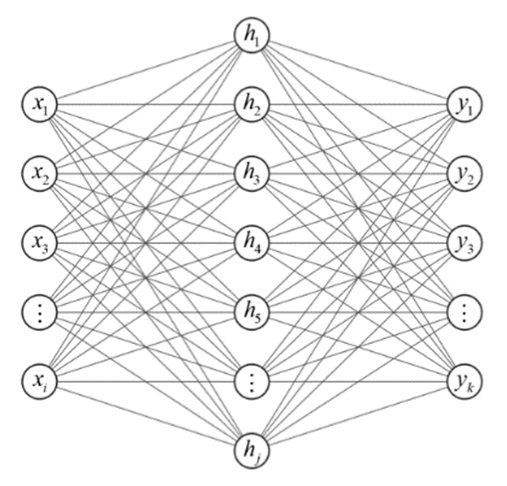
Figure 2.
Common activation functions listed as follows: (a) relu function; (b) sigmoid function; (c) tanh function; (d) softplus function.
Figure 2.
Common activation functions listed as follows: (a) relu function; (b) sigmoid function; (c) tanh function; (d) softplus function.
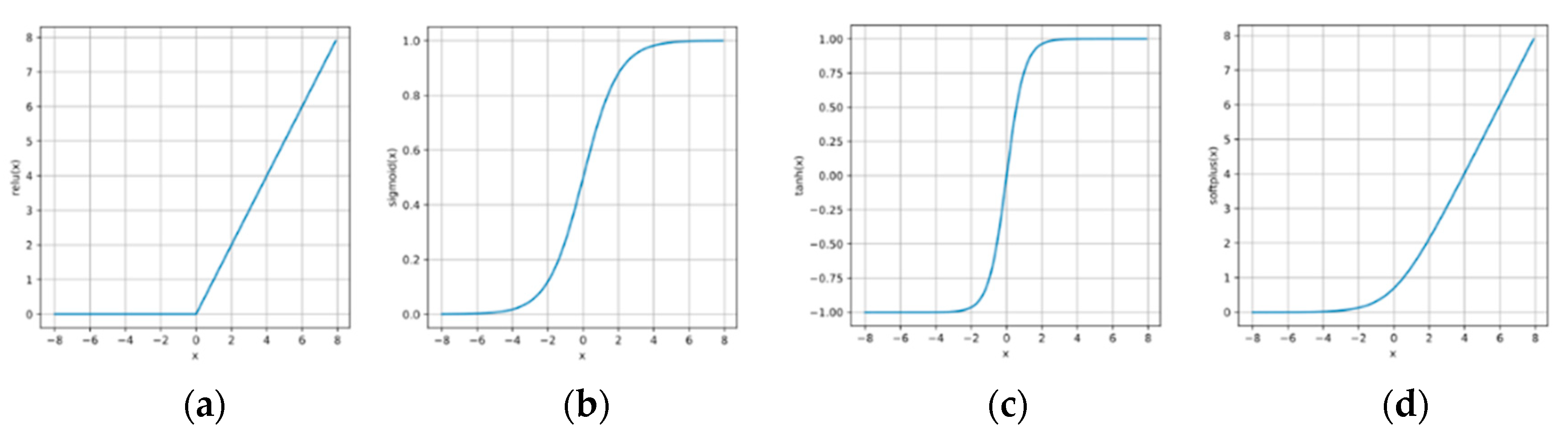
Figure 3.
A tightly stretched wire under loading.
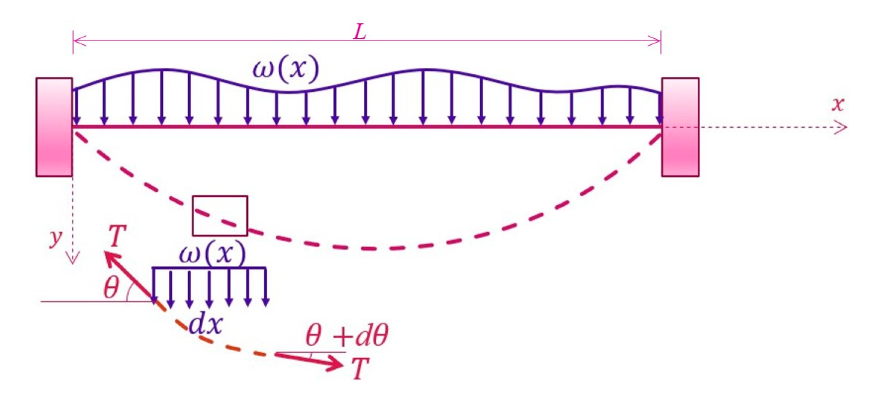
Figure 4.
The convolutional neural network scheme for the tightly stretched wire problem.
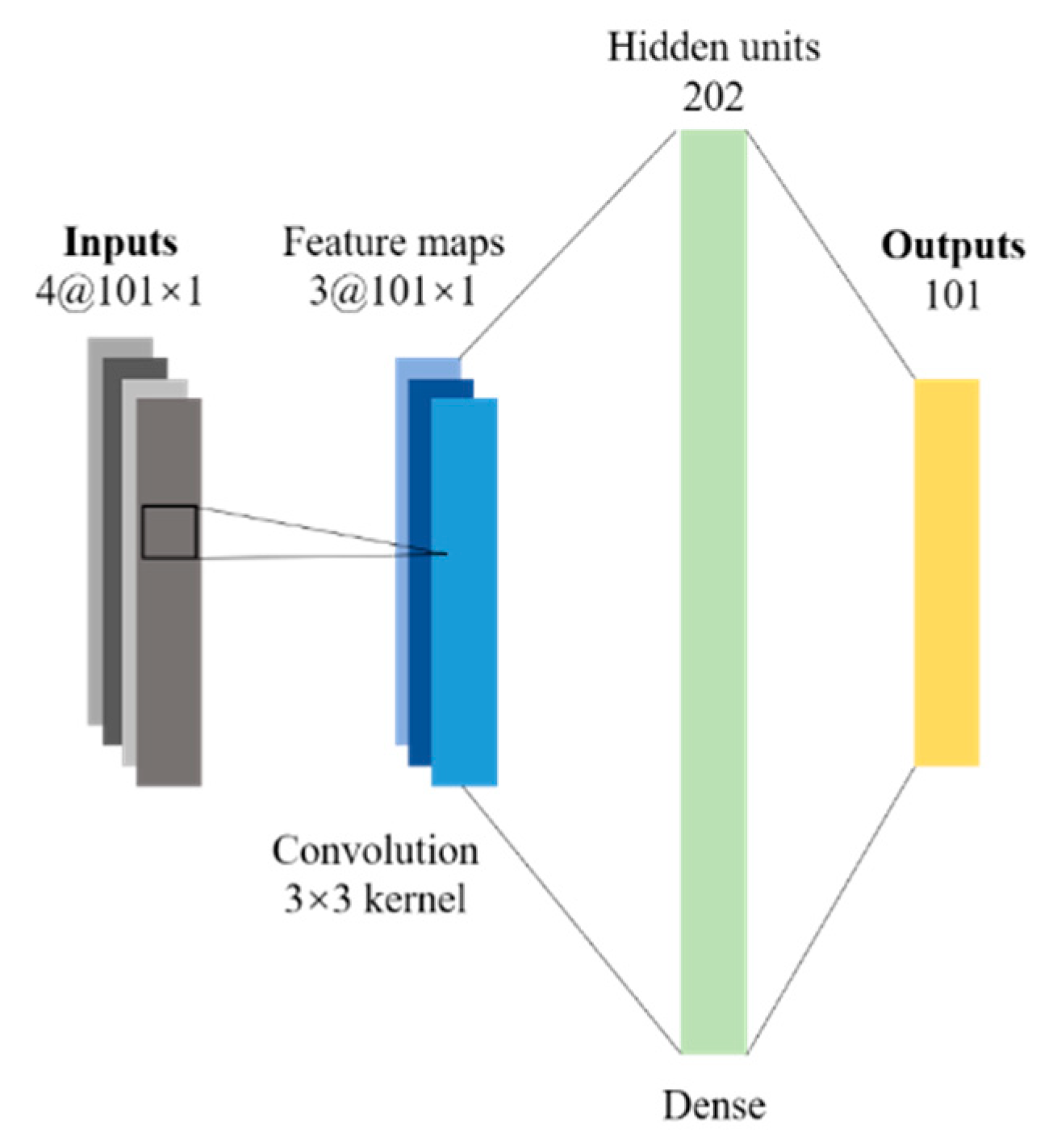
Figure 5.
For three cases (A, B, C), MSE of the test set for different neural networks.
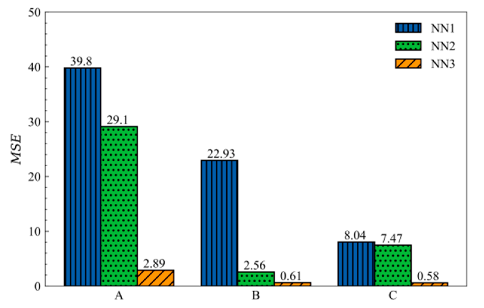
Figure 6.
The three samples with the maximum error in the test set (The green bar chart above the x-axis represents the magnitude and location of loads).
Figure 6.
The three samples with the maximum error in the test set (The green bar chart above the x-axis represents the magnitude and location of loads).
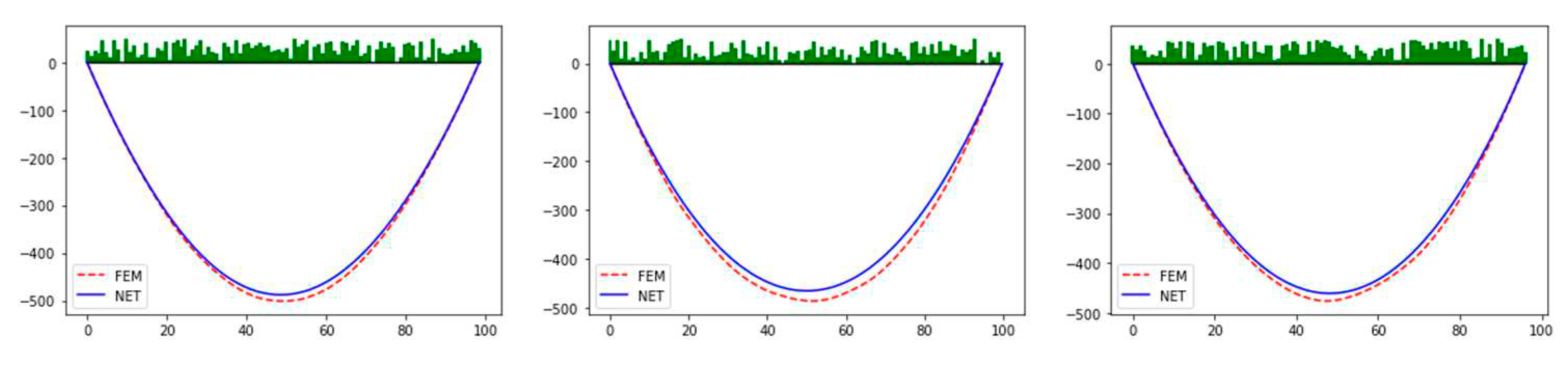
Figure 7.
Notable samples in the test set (The green bar chart above the x-axis represented the magnitude and location of loads).
Figure 7.
Notable samples in the test set (The green bar chart above the x-axis represented the magnitude and location of loads).
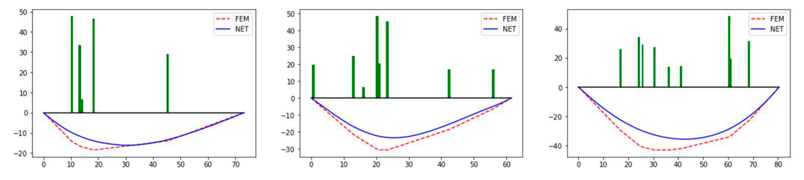
Figure 8.
A concrete gravity dam.
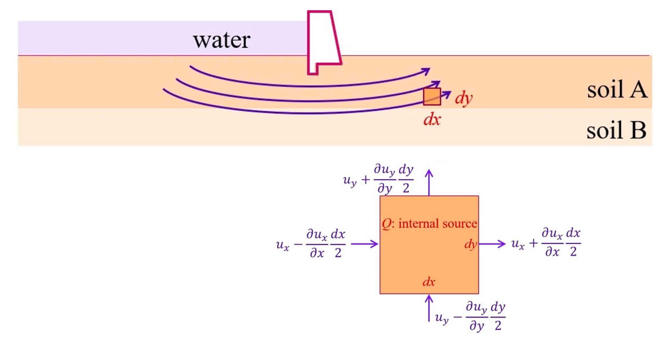
Figure 9.
The configuration and mesh of the concrete gravity dam.
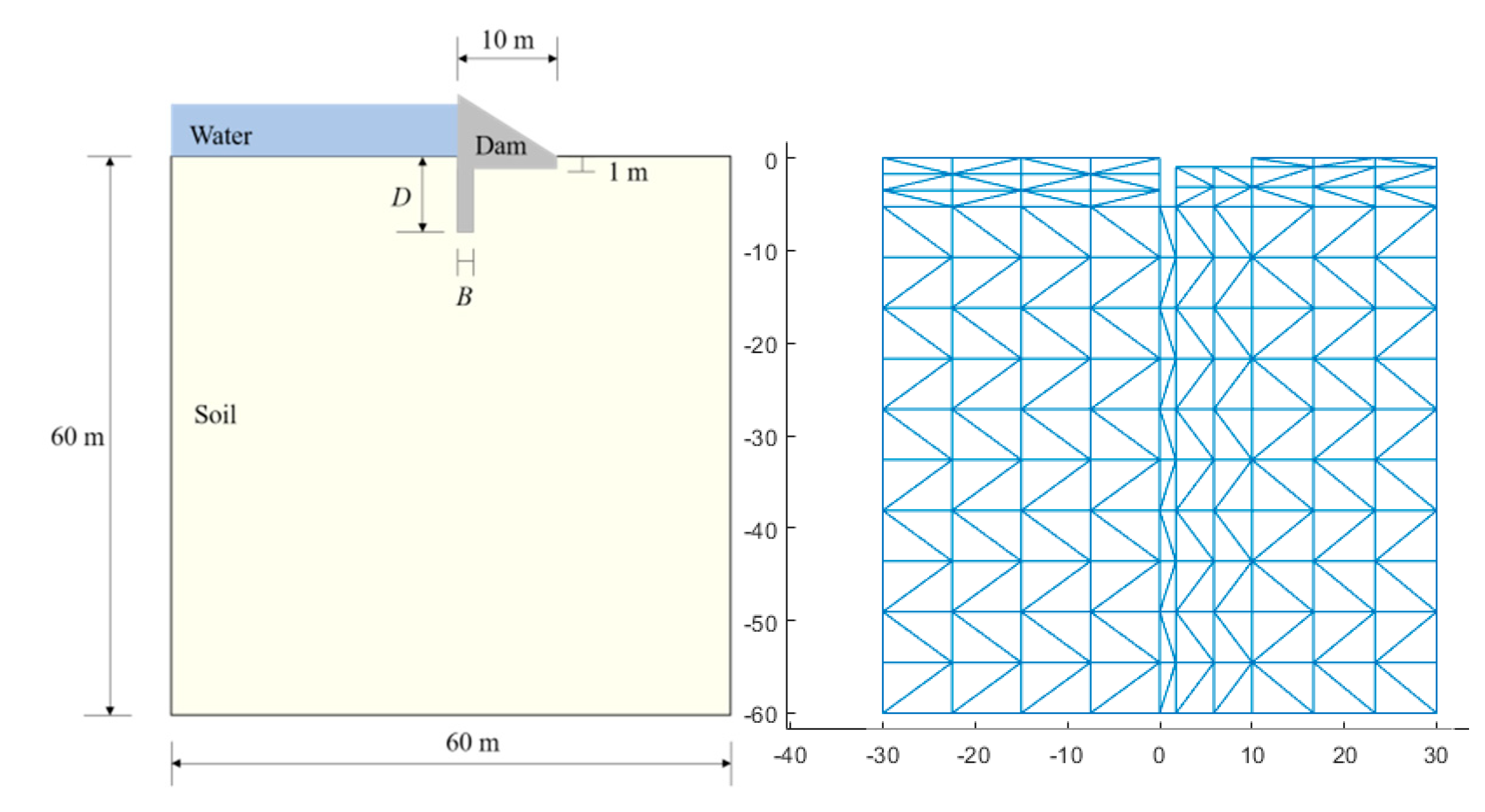
Figure 10.
Four samples randomly chosen in the test set: (a) constant heads; (b) impervious boundaries.
Figure 10.
Four samples randomly chosen in the test set: (a) constant heads; (b) impervious boundaries.
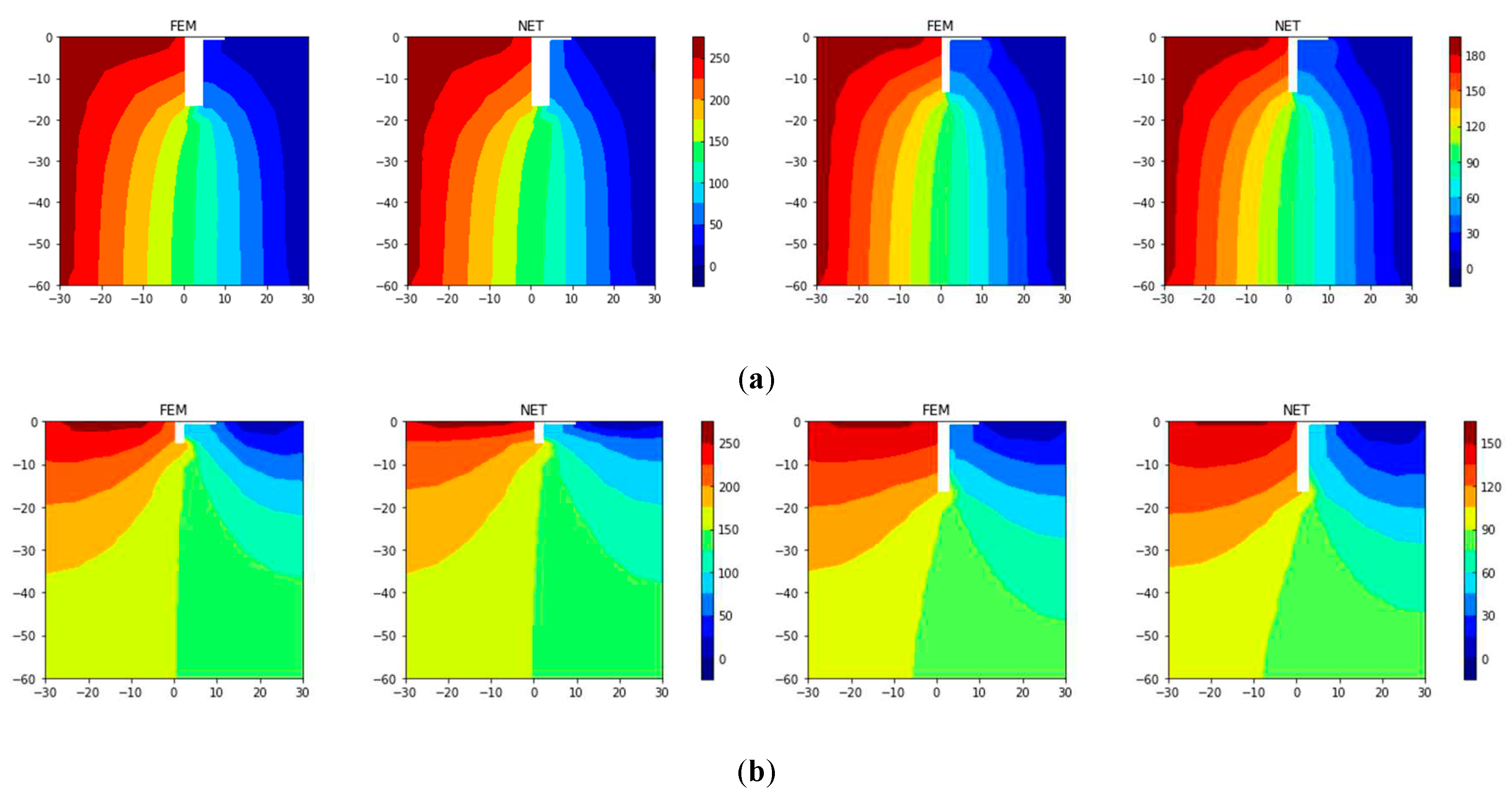
Figure 11.
A two-dimensional cantilever beam subjected to a uniform downward loading at the free end.
Figure 11.
A two-dimensional cantilever beam subjected to a uniform downward loading at the free end.
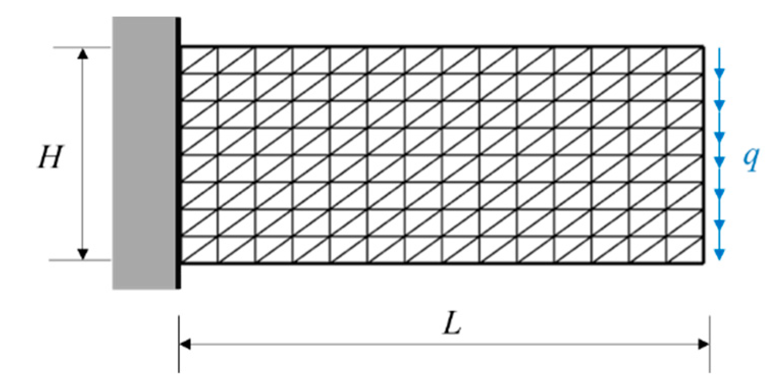
Figure 12.
A comparison between solutions from FEM and ones of neural network for the cantilever problem.
Figure 12.
A comparison between solutions from FEM and ones of neural network for the cantilever problem.
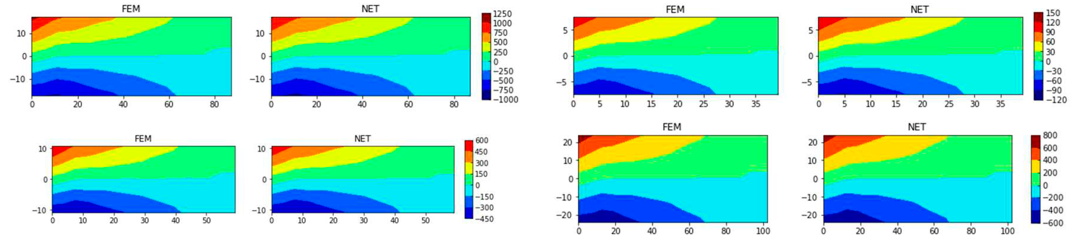
Figure 13.
A sample in test set with SMAPE 18.11% and MAPE 3.24%: (a) solutions from FEM and ones of neural network and (b) SMAPE distribution
Figure 13.
A sample in test set with SMAPE 18.11% and MAPE 3.24%: (a) solutions from FEM and ones of neural network and (b) SMAPE distribution
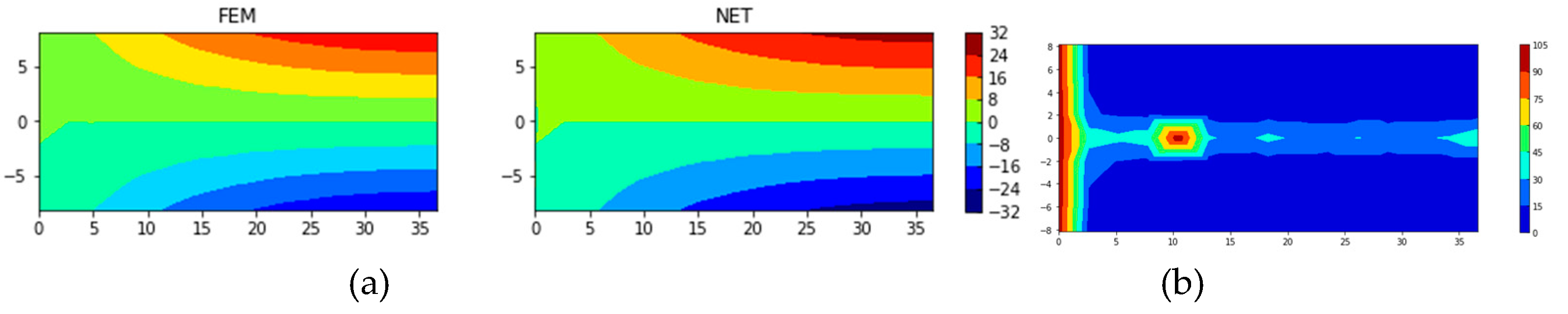
Figure 14.
A simply supported beam was subjected to a uniform load from the top.
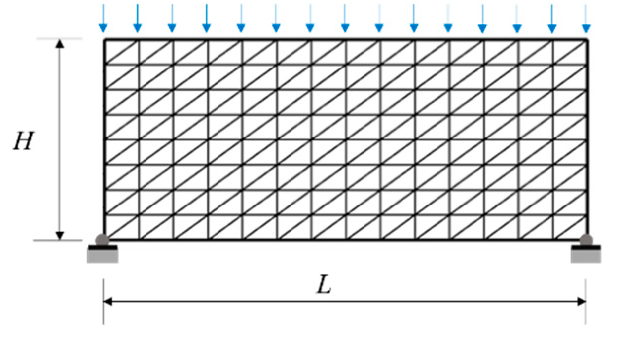
Figure 15.
Comparison between FEM and NET for several samples in the test set of (a) σxx and (b) σyy.
Figure 15.
Comparison between FEM and NET for several samples in the test set of (a) σxx and (b) σyy.
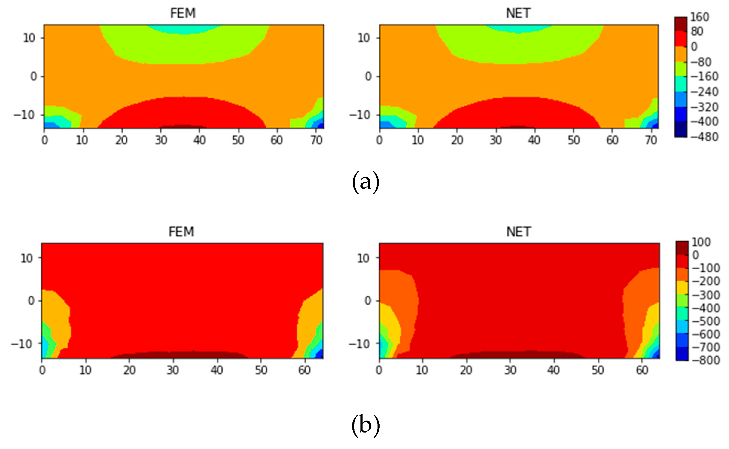
Figure 15.
Comparison between uy solutions from FEM and ones of neural network for the beam.
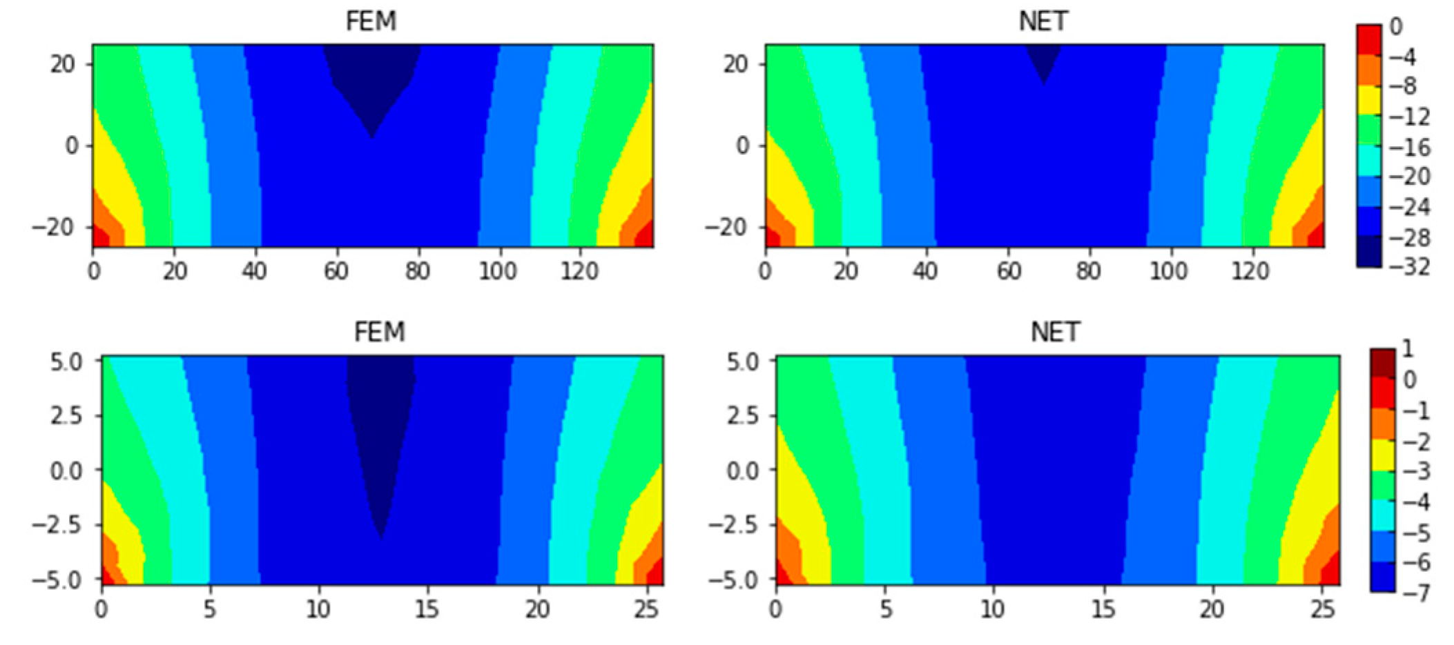
Figure 16.
Configuration and mesh of the plate with notches.
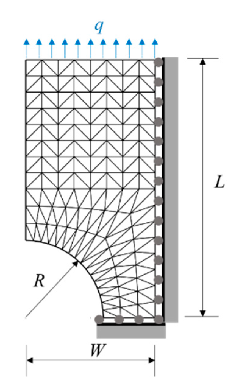
Figure 17.
Comparison between σeff values of FEM and ones of neural network.
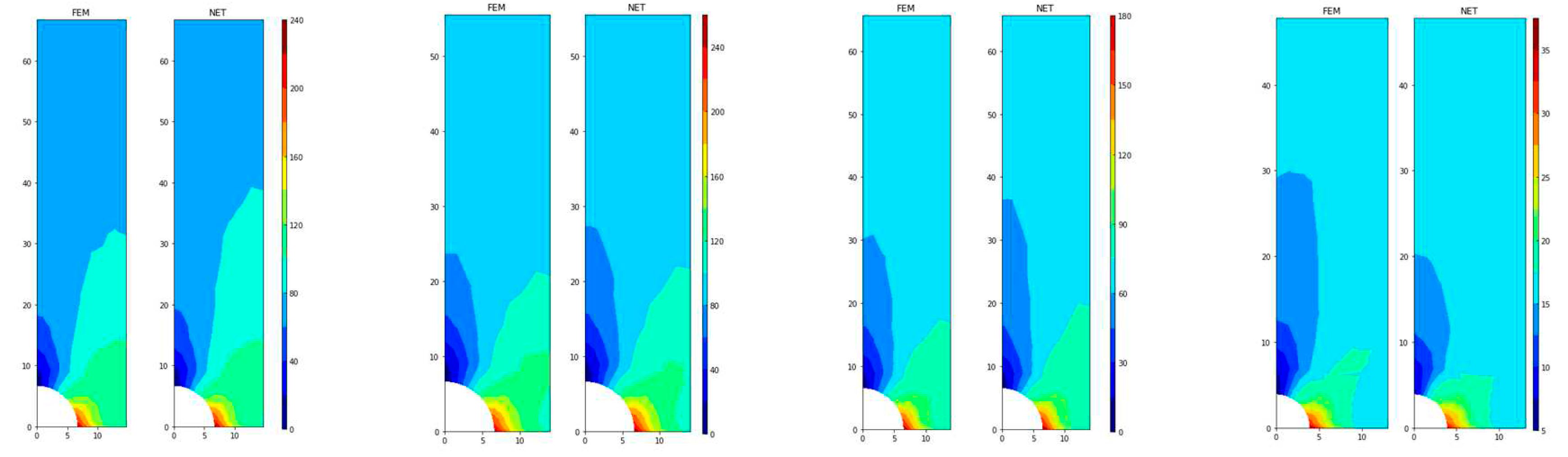
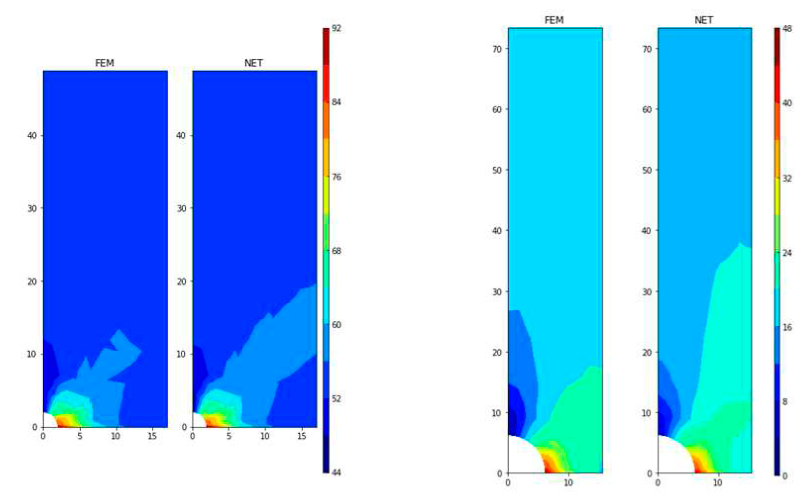
Figure 18.
Comparison between uy values of FEM and ones of neural network.
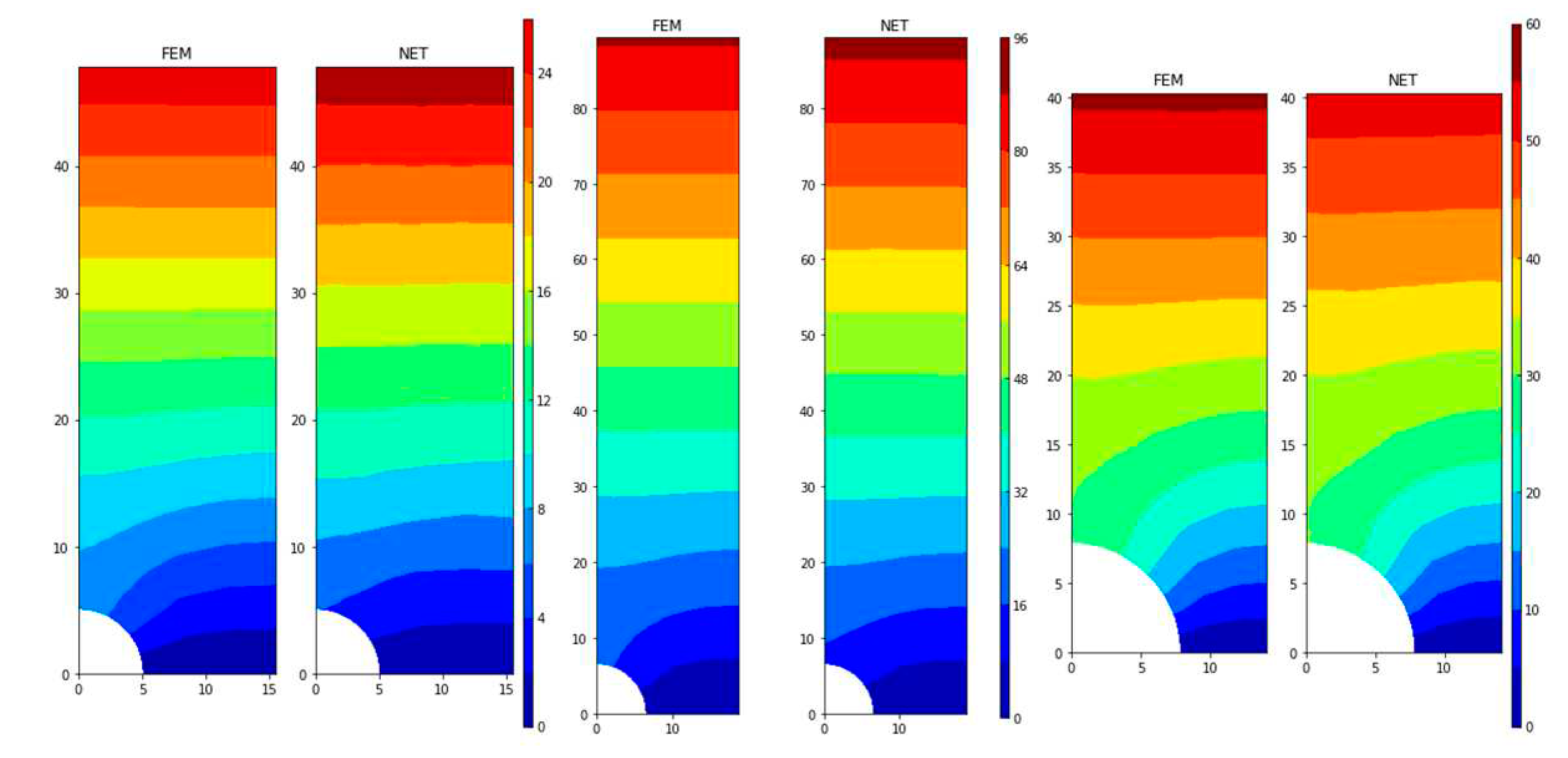

Table 1.
Values of FEM parameters given in the flow through porous media problem.
| D (m) | B (m) | R (m/day) | (m) | |
| Minimum | 5 | 1 | 0 | 5 |
| Maximum | 20 | 5 | 0.5 | 30 |
Table 2.
Minimum and maximum values of FEM parameters for the cantilever beam.
| H (m) | L (m) | q (N/m) | E (Pa) | v (-) | |
| Minimum | 10 | 2H | 0 | 1×10⁶ | 0 |
| Maximum | 50 | 3H | 100 | 1×10⁷ | 0.5 |
Table 3.
Minimum and maximum values of FEM parameters for the plate with notches.
| R (m) | W (m) | L (m) | q (N/m) | E (Pa) | |
| Minimum | 1 | 10 | 2×W | 10 | 1×10³ |
| Maximum | 8 | 20 | 5×W | 100 | 1×10⁴ |
Disclaimer/Publisher’s Note: The statements, opinions and data contained in all publications are solely those of the individual author(s) and contributor(s) and not of MDPI and/or the editor(s). MDPI and/or the editor(s) disclaim responsibility for any injury to people or property resulting from any ideas, methods, instructions or products referred to in the content. |
© 2023 by the authors. Licensee MDPI, Basel, Switzerland. This article is an open access article distributed under the terms and conditions of the Creative Commons Attribution (CC BY) license (http://creativecommons.org/licenses/by/4.0/).
Copyright: This open access article is published under a Creative Commons CC BY 4.0 license, which permit the free download, distribution, and reuse, provided that the author and preprint are cited in any reuse.


