1. Introduction
Since its inception in 2015 [
1], deep reinforcement learning (DRL) has found many applications in a wide set of domains [
2]. In recent years the use in trading has become quite popular, at least in academia (for an overview, see [
3] or [
4]).
The most interest lies with the portfolio optimization problem (see, for example, [
5,
6,
7] for some modern approaches), which can leverage multiple assets both in uptrend and downtrend. In single-asset trading, there is too much risk involved, as argued in, for example, [
8], if the asset goes down, then the best option is to hold. Also, if the market is in a strong bull trend, it is hard to beat it, see for example a recent confirmation of this by [
9]. The market (in this case, the single asset) often changes regimes regarding volatility, trend, smoothness, etc. There have been many works showing and modeling this, see for example, works mentioning
trading and
market regime switch (e.g., [
10,
11]).
The applied methodology pursued by many researchers working in DRL for trading (if not all) is to evaluate the agent for some short period (test mode) and then retrain it to deal with another test period. Moreover, the training must occur before the testing so the agent can catch the current market dynamics.
This workflow is cumbersome and introduces additional constraints and computational costs. Moreover, the uncertainty about the change in the market regime and timing still needs to be addressed in real-time. We thus propose an alternative method, where a hierarchical system decides which of the regimes the market is in and assigns the most appropriate behaviour by selecting a low-level agent to act in the actual market, i.e., buy and sell the asset. We delve more into the architecture in subsequent sections. We now proceed to the RL problem formulation.
The reinforcement learning problem is usually formulated as a Markov Decision Process (MDP)[
12], which is a discrete stochastic control process for decision-making in environments with uncertainty (there are also continuous MDPs [
13]). Formally, a discrete MDP is given by:
a set of discrete states the agent can be in, often called the state space
a set of discrete actions the agent can take in the environment, also referred to as the action space
which is the probability of being in state s at timestep t, taking an action a and then being in at timestep . This formulation is also known as the transition function.
, which is the reward function, similarly dependent on a the current action, and s, the current state and is given by the environment when in the next state . Usually, the policy of selecting an action a when in state s is denoted by and is often probabilistic.
In dynamic programming, which is somewhat the precursor of RL, where the transition function and reward function are given or known, two equations are employed alternatively:
to update a value function which encodes how good it is to be in state s
and to update the policy which reflects the value function and it is taken to be the action which maximizes this value function estimate, known as the greedy policy for V
Formally:
where
is called the discount factor and
. A commonly used RL alternative is to use a state-action value function where now we have two identifiers,
s and
a, where
p and
r are unknown:
with the model-free, the iterative version given by (which is, in a sense, an approximation of the above equation with the greedy policy selection step included):
There are two classes of algorithms for RL, value function algorithms, which try to estimate the state-value function V accurately, or the state-action value function Q (Q-Learning), and policy algorithms which look directly at optimizing (policy gradient), bypassing the value function estimation (others are using both methods, e.g., actor-critic).
On a different set of axes, there are model-based RL agents that model and learn the transition function and are model-free, which do not explicitly model the transition function. Model-based RL implies the existence of a simulation of the environment with which the agent can interact without incurring the cost associated with or benefiting from the precision of the real environment. If a model can learn accurately and efficiently, then the advantages of having a model are apparent; knowing the possible outcomes of some actions without actually taking them enables long-term planning and significantly enhances the agent’s capabilities.
Instead of using the summation over all possible following states to get a value for
Q, we concatenate the prediction of the next state(s) to the current state, effectively adding another identifier to the
Q function, which is the predicted future. This approach is more efficient and less accurate but still uses the information from the prediction. Moreover, it can be applied to any reinforcement learning algorithm with minimum overhead. This methodology has been used with the same purpose, see, for example, [
14]. This technique could be classified by [
15] as implicit model-based RL, where we do not explicitly model the transition function and the planning procedure, but we use the prediction as part of the RL agent representation.
2. Related work
The idea of having an environment model has been used in the past quite effectively, both with analytical gradients [
16] in the linear regime, and even neural networks [
17] in the nonlinear. As long as a model can learn to some degree of accuracy, and it is not too computationally intensive to do so, then the use of a model generally improves performance and sample efficiency. Moreover, it gives the ability to generate or roll out future trajectories.
This ability is instrumental in trading, where accurate predictions could greatly enhance profits, especially if they are multi-step. A couple of recent works combine DRL and MB methods for trading [
14,
18]. In [
18], they use a sequence-to-sequence RNN-MDN (mixture density network, [
19]) to model the transition model based on latent states given by a convolutional autoencoder. They show that the performance of an agent trained on the transition model is very similar to the one trained on the actual data, with the ability to explore the transition model and exploit it using the real environment. In the second work [
14] using model-based prediction with DRL for trading, the authors use a Nonlinear DyBM (Dynamic Boltzmann Machine) to make predictions and embed these into the state of the agent; they call it infused prediction module.
On the other end, hierarchical RL enables the partitioning of the state space in some meaningful way (usually done automatically) and solving different problems individually with the so-called skills or options, sub-policies directly interacting with the environment. A higher-level agent chooses between these sub-policies according to some criteria and stops them according to some termination function, simultaneously giving goals and rewards to the low-level agents. Some of the new approaches to HRL using deep networks can be found in [
20,
21,
22]; however, the concepts are much older, see [
23,
24]. For a more detailed overview, see [
25]. The goal is to learn specific behaviours well while combining the learned solutions adaptively. Hierarchical RL methods hold promise for general artificial intelligence. In trading, they have been used successfully, for example, in portfolio management [
26,
27], but not in the single asset case.
The association of hierarchy with model-based RL seems fruitful; however, only a few works exist combining the two. It has been mentioned as the promise for the future in [
28] but more from a philosophical or cognitive point of view than from a practical, applied to a real-world problem. More recently, the association has been done in [
29], which uses inductive logic programming to devise a transition model. It combines symbolic representations by employing an additional symbolic MDP, which augments the state with boolean predicates, which can be goals, the relationship of objects, events, or properties in the environment. The rewards for the low-level agent are augmented with some positive number if the agent reaches the subgoal given by the high-level agent (using the symbolic transition model), which uses as a reward the accumulated environmental rewards when the low-level agent reaches the subgoal and small penalizing factors for giving immature and unlearnable tasks as subgoals. The high-level agent alternates interacting with the environment and the simulated transition model, which results in increased sample efficiency. The overall agent is tested on two hard environments for flat agents (not using hierarchy), showing good performance. It is unclear if for both, but for one environment (involving a robot reaching several circles in a specific order), the HRL uses a tabular Q-learning for the high-level agent and a PPO agent for the low-level. Even though it is partly a symbolic approach and thus significantly engineered, it shows the potential of combining hierarchy and explicitly learning a transition model.
Our architecture is similar to the options framework [
30], where an option is defined by:
a set of initial states from which an option o can be started, with
a policy which is followed for the duration of the option
a termination function that governs the termination of the policy when certain conditions are met
We describe our architecture and how the above points correspond to it.
3. Overview
We combine the model-based approach with a hierarchical structure, such that we use a high-level agent to select among a set of pretrained low-level agents, then act for several steps in the environment. These steps are governed by some termination function
, which in the simplest case is given by:
where % is the modulo operator,
s is the current state,
t is the current timestep in the environment, and
k is some value significantly larger than 1; this is the resolution at which the high-level agent sees the world, the subsampling factor. We set
(we test for
). The options’ policies are the actual low-level policies pretrained beforehand or simple strategies governed by some technical indicators (like moving average crossover or mean reversion strategy). We use 5 PPO agents and two simple strategies. The initiations sets are all the same for all low-level agents and are constituted by this reduced set
, which comprises every
element of
, with
.
The high-level agent is endowed with a classification mechanism
, which clusters incoming series into different classes and feeds different agents with samples from these different clusters. This mechanism is analog to the subgoal discovery problem [
31,
32], where a similar processing exists, where the high-level agents find attractive states for the low-level agent to reach. Because the environment is different in our c, reaching the subgoal does not have any real meaning to it. We use
[
33] from the Python library
1 for clustering the time series, with an episode length of 50 and 5 clusters. We tested more clustering algorithms, but they all gave similar results, so we chose the simplest one. We also tested more values for the number of clusters, but we chose a small one that showed the significant trends one can see in a market.
We already see how model-based prediction can help. By assigning an agent to act for the next window, we have to classify it as being in one of the clusters, which means we first have to predict it and then classify this prediction to match the agent. We denote by
f the prediction function for the high level and by
g the prediction function for the low level. For
f we use a deep autoregressive model using recurrent neural networks [
34] from the Python library
gluonts 2, which is a probabilistic time-series library focused on deep learning models. For
g we use a Dynamic Boltzmann Machine
3 which is generally good for 1-step prediction and also has a constant training time.
For the RL part, we use
RLlib 4, which is a Python RL library that scales very well on multiple CPU cores and machines. It also has the latest state-of-the-art algorithms and RL tricks implemented and ready to use.
3.1. Data
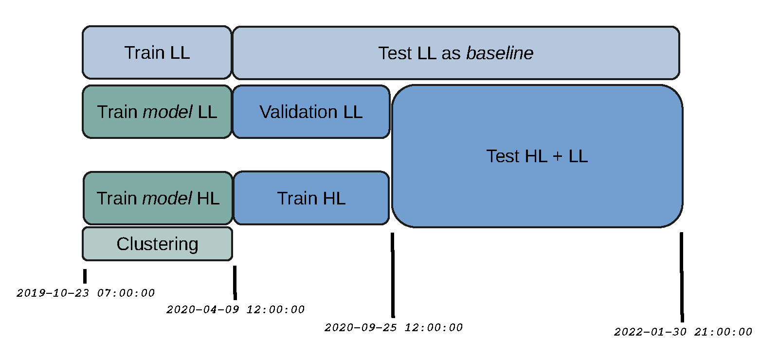
We sample data at 1 hour (1h) frequency and use 4000 data points for training the low-level, 8500 points for training the high-level (including the previous 4000), and 10000 points for testing (BTCUSDT taken from Binance, 2019-10-23 07:00:00 - 2022-01-30 21:00:00). For details on the data splits see
Figure A2. For training the low level we sample episodes of length 50. For the high-level, we use 1500 (which amounts to 50 decision points for the high-level agent since it acts every 30 steps). For each performance measurement, we take 30 random samples.
Here we deviate from the general literature, where the test sets are much smaller than the training sets, and often each testing set has to be preceded by a training set due to what is considered a requirement due to the nature of the market and its different regimes. It is assumed that for an agent to perform well on some data, it needs to be trained on the period right before that. Because we deal with the different regimes in another way (by employing heterogeneous agents), we can train systems that perform well on an extensive testing set and do not need to be trained multiple times for each testing period. Our agents are general enough to deal well with any market regime.
For the low level, the data is concatenated as , where corresponds to the last n steps of the respective price return (open, high, low, close). By price return we mean that . is the volume associated with timestep t, and is also a normalized difference: .
3.2. Architecture
After we tried running multiple types of agents on the various parts of the dataset and obtaining poor performance, we noticed that the performance was correlated with the training data; thus, we concluded that partitioning the data in some meaningful way might be fruitful. We describe this next.
The preprocessing for the high-level agent is done by the clustering mechanism, where we classify each running episode in one of the existing clusters (
) and feed as state the last
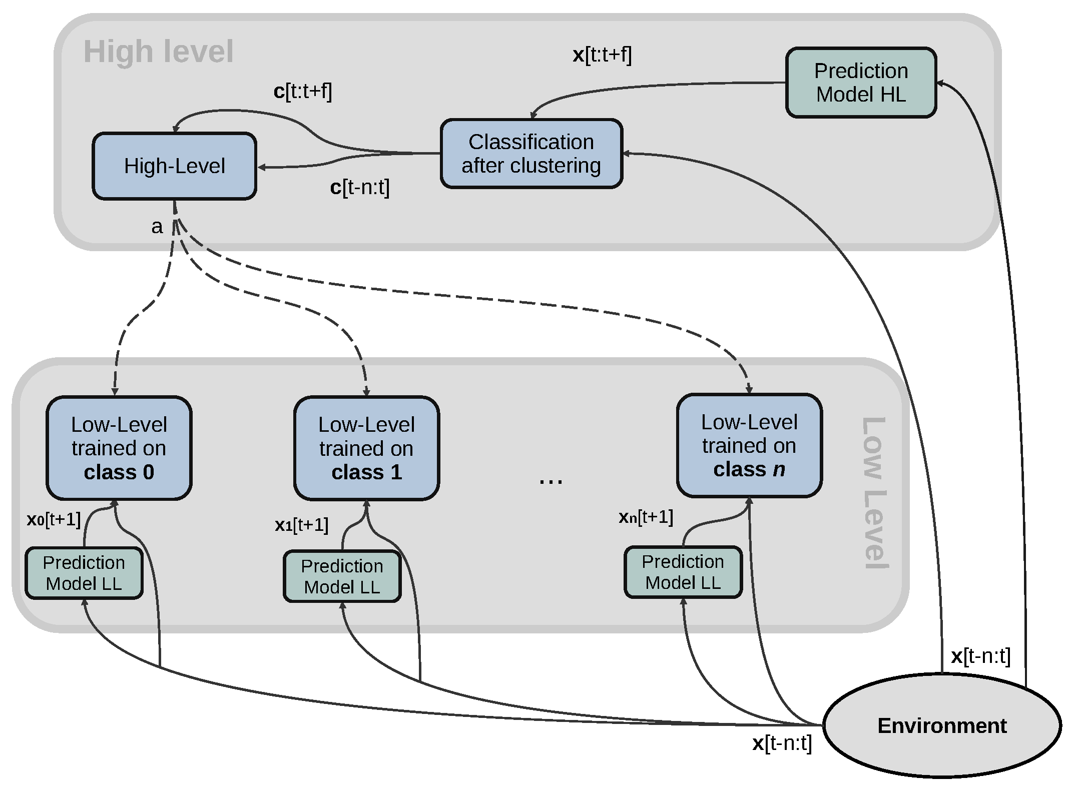
n such classifications. To select the low-level agent to act, we consider this representation more appropriate since the classes represent the expertise of each agent in some sense. Moreover, neighbouring episodes will have the same class, thus inducing smoothness in the representation and thus action selection, which is in line with our goals. We show the overall architecture of our learning system in
Figure 1.
Figure 1.
Depiction of the overall architecture.
Figure 1.
Depiction of the overall architecture.
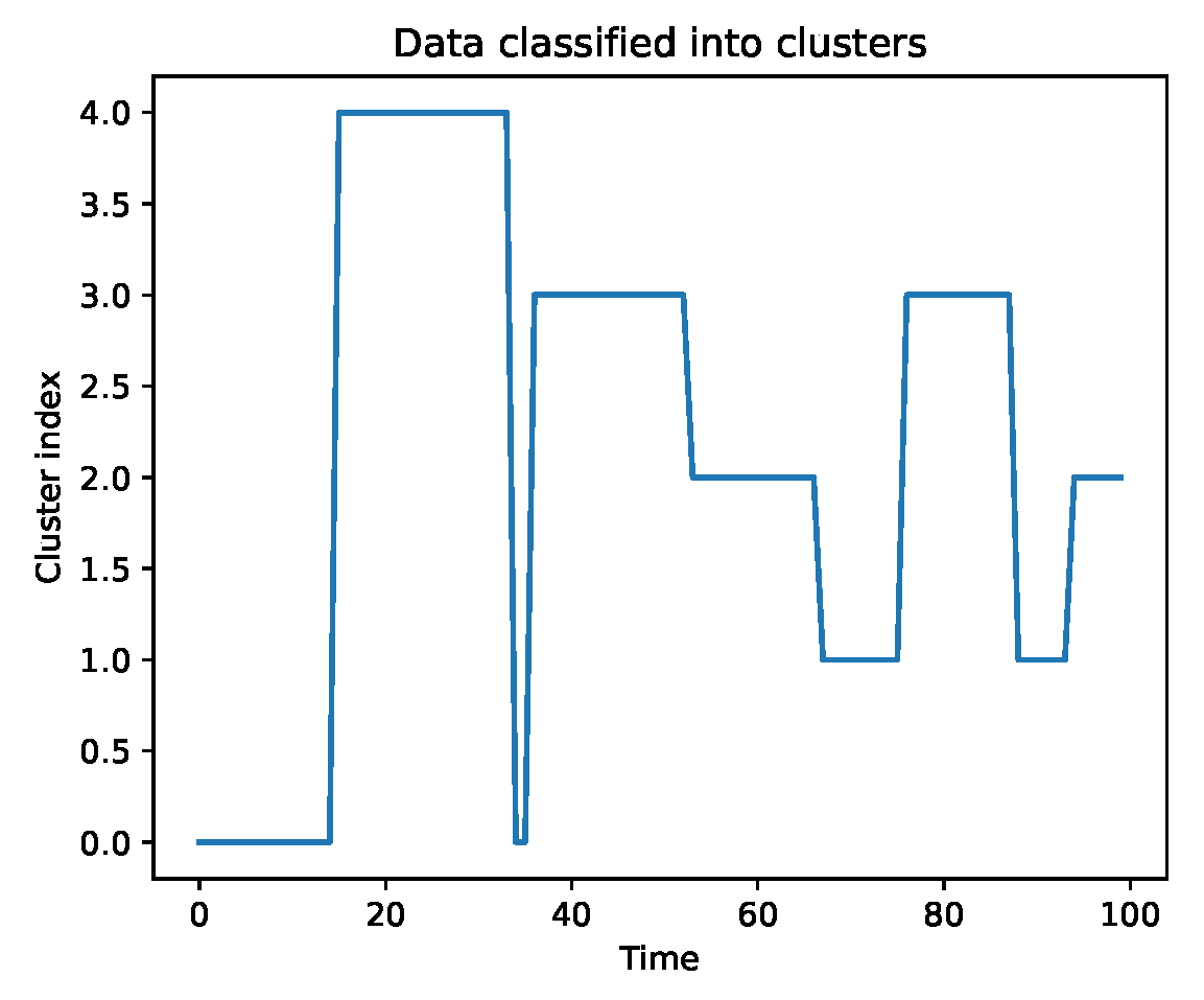
Figure 2.
State representation for the high-level agent.
Figure 2.
State representation for the high-level agent.
The low-level prediction did not improve much (or at all, the results were inconclusive) the performance of the low-level agents; thus, we do not include it in the final results. Looking at the low-level prediction in
Figure 5b, a more accurate prediction model is needed. For the high-level state, we tried multiple approaches:
using raw returns as in the low-level agent
using the recent performance of each individual agent in its own simulated environment (similar to [
7]) and concatenating these for all agents
using concatenated samples from the prediction model instead of median or mean
using the result of the classification of the recent past and the prediction, applying
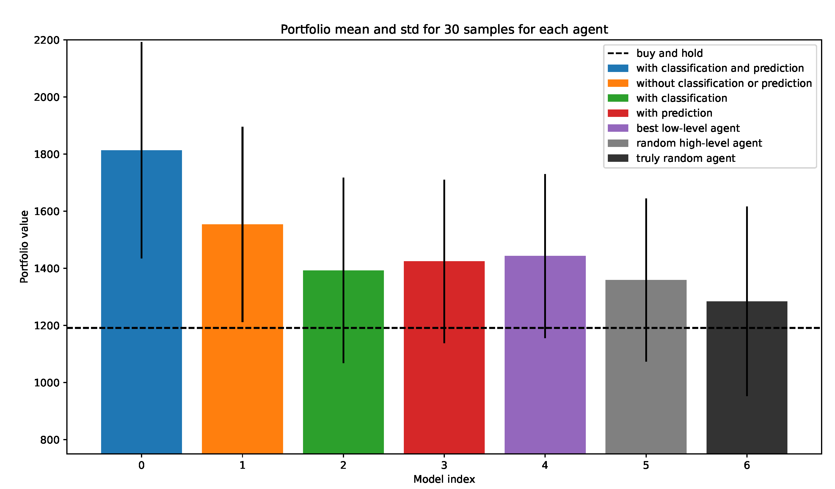
The best version used both classification and prediction, see
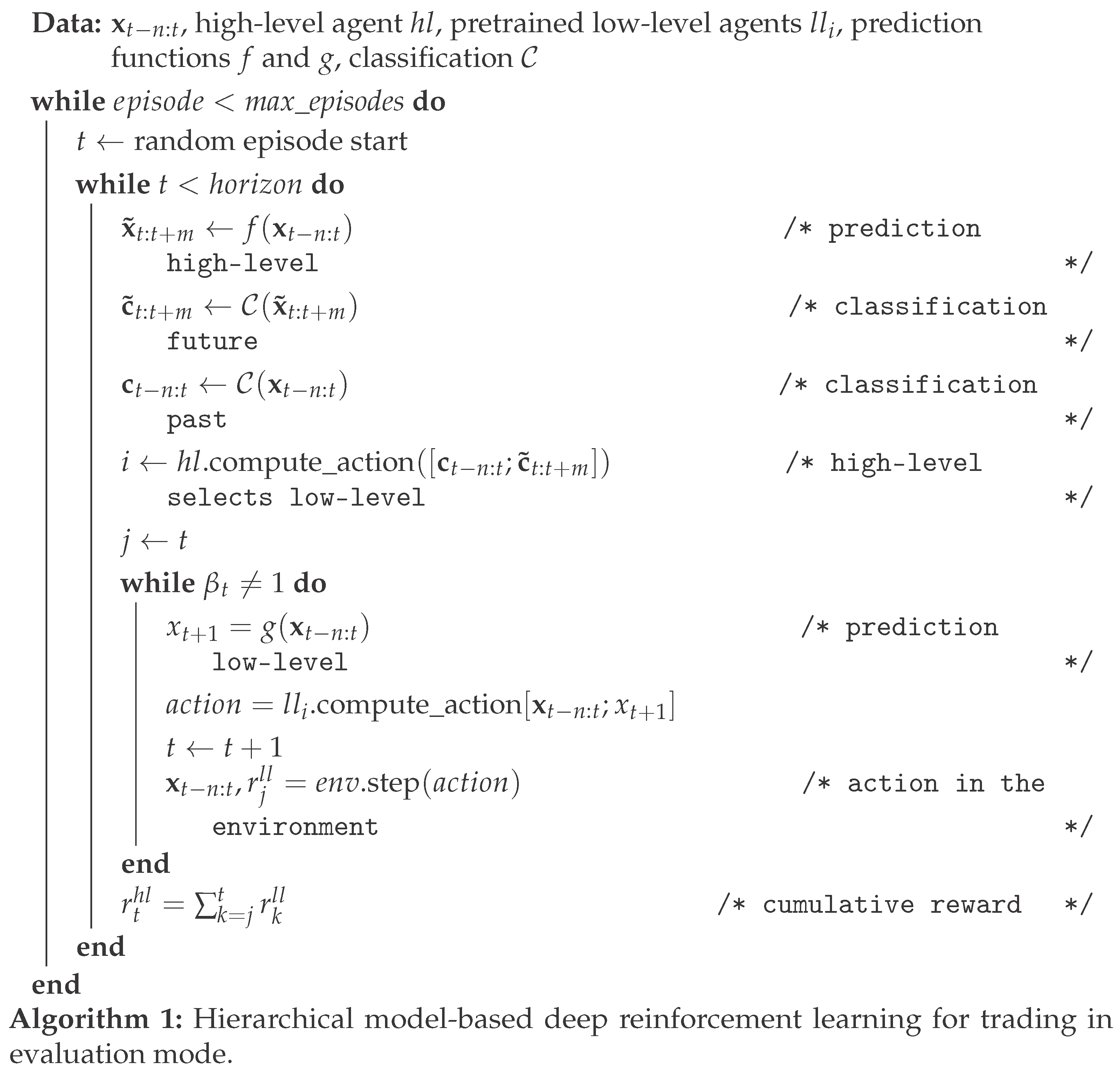
Figure 7. In general, larger state spaces induce more variability, in our experience, which is also what happened when using raw samples from the prediction model. We show the full algorithm in Algorithm 1.

3.2.1. Clustering as preprocessing for the high-level agent
We endow the high-level agent with a preprocessing module that can cluster the incoming time series into a specific cluster (one of 5 discovered beforehand when clustering the training set, see
Figure 3).
Figure 3.
The 5 clusters discovered.
Figure 3.
The 5 clusters discovered.
We denote by
the state of the high-level agent. The state at timestep
t is given by
where
is a vector of the last
n classifications, where each point
with
denotes the classification of the episode which ends at
.
is the prediction of the following episodes classes by the classification, which is fed with the prediction of the next timesteps. Thus, each point
with
, is the classification of the (predicted) episode ending at
. Because the high-level takes decisions at a coarser data granularity, having such a multiple-step prediction model makes sense. We use a DeepAR model for our multiple-step prediction, which generally keeps the shape of the future trend but lacks minute precision, which is what we needed. We show example predictions in
Figure 5a.
3.2.2. Pretraining the low-level agents
We pretrain the low-level agents on specific data clusters, so each one specializes in one type of trend. We show the clusters and their means in
Figure 3. We see that the 5 clusters catch some of the main trends in the market.
Figure 4.
Performance of the low-level agents, each trained on one cluster.
Figure 4.
Performance of the low-level agents, each trained on one cluster.
We show
Figure 4 the best performance of individual agents on the test set consisting of 15000 points (21 months). We select the best one (among 24 trials) for each class for comparison. We perform 30 repetitions for each and depict the mean and standard deviation.
3.3. Prediction
In the context of RL, prediction assumes the existence of a model of the environment with which the agent can interact without incurring the losses associated with the real environment. This complete model comprises state and reward models, predicting the following states and rewards. We are only interested in the state model, as the reward model is completely dependent on the state model. In the sense that if we know the next state (price) we can easily compute the rewards, given the action taken.
Figure 5.
Sample predictions.
Figure 5.
Sample predictions.
For the low-level, we tested with the true values instead of the predictions to see if the performance improved. We noticed a significant improvement. We repeated the value of the future step 10 times and then concatenated this to the state vector for the low level as a way of biasing the agent, such that this future value has a more considerable influence on the decision (having a single value did not seem to work too well). So it is clear that accurate predictions can significantly improve performance and training time. We thus add a 1-step prediction for each of the OHLCV time series, thus having five different prediction models for each agent. As we mentioned, this does not improve performance conclusively.
For the
high-level agent, the representation is in terms of classes (0 to 4), and thus the prediction should be the same. We also note that the history window size has now doubled compared to the low-level since an episode now defines every point
ending at that point. So we predict multiple steps into the future and look at more steps into the past. We show an example in
Figure 2.
3.4. Rewards
The rewards for the low-level agent are given by the usual profit and loss (PnL). We also standardize the rewards, subtracting the running mean and dividing by the running standard deviation of the current episode at each step. We do this operation for all types of rewards used and all agents.
For the high-level agent, we feed the cumulative profit and loss for each low-level episode, while for the low-level, we feed the realized PnL (profit and loss):
where
is the first open buy price, see Section 7.1.
3.5. Termination function and diversification
By looking at the low-level agents’ pretraining performance, we can draw some conclusions:
if a large loss has been incurred, there are chances that this is a period of losses for this agent (and not only; we see that some periods of losses coincide for all agents). Thus we add a hold action for the high-level agent.
recent agent performance could be relevant for the immediate future
agents are not complementary, but combining more of them can bring improved performance
improving diversification in the low-level dynamics might improve overall performance
We hypothesized that the termination function would be necessary for trading and that the overall strategy could be improved by learning when to terminate, but it seems not. We tested with multiple values (10, 30, 300), and the difference is small, especially among lower values. We settled on 30 as the value, which seemed more robust.
4. Experiments and results
Firstly, we have also to mention the usual RL instability in training and emphasize how best hyperparameters were different in each selection (for the pretrained agents or the hierarchical agent), so running multiple trials with different configurations of hyperparameters at each experimental stage is critical for obtaining reasonable solutions. We evaluate 30 samples for each curve after an initial run of 24 trials and selecting the best hyperparameter configuration. A significant improvement was also adding the ability to hold (or do nothing) for the high-level agent, thus for a more extended period (the terminating value k), which makes sense because, as we saw from the low-level pretraining, there are extended periods where it is better to do nothing, as it is almost impossible to be profitable.
Performance gains were hard to obtain with this setup, due to the fact that agents were not very dissimilar when making profits, thus we wanted to add more agents, but with different trading dynamics. We proceed to describe these steps.
4.1. Hierarchy with two simple strategies
We test two basic strategies, a mean reversion and a moving average crossover, which can be considered a momentum strategy.
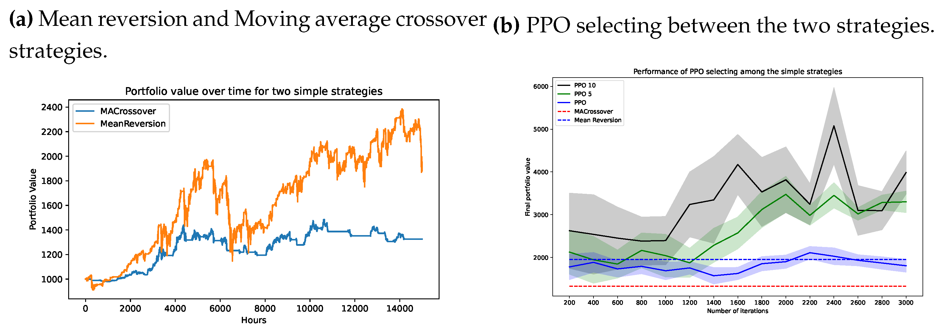
Figure 6 shows the performance of the two basic strategies. We then check to see if using a DRL agent to select between the two strategies is of any help. We also add the hold option for the agent to choose from three discrete actions. We show the performance of the DRL agent (we use a PPO agent as before) in
Figure 6. We see that performance is indeed better than each of the two individual strategies. We use a minimal
network with a
activation function. We try three decision intervals for the PPO: every step, once in 5 steps (PPO 5), and once in 10 steps (PPO 10).
The mean reversion strategy uses two indicators, a Relative Strength Index indicator with an exponential moving window working on a period of 6 hours and a moving average on a period of 20 hours. The strategy buys if the RSI value is less than some threshold (40 in our case) and the price value is less than the lower Bollinger band and sells if the RSI value is higher than some threshold (60 in our case) and the current price is higher than the higher Bollinger. The higher and lower Bollinger thresholds are at , with the rolling standard deviation of the time series (on the same period as the mean, 20 hours). The strategy holds or does nothing if none of the above conditions are met.
The moving average crossover strategy is even more straightforward. We have two different moving averages (in our case, one works on a 100 hours window and the other on a 400 hours window), and when the shorter one surpasses the lower one, it is a buy signal, and when the reverse is the case, that is a sell signal.
Figure 6.
Performance of a hierarchical agent (PPO) using two basic strategies as low-level agents.
Figure 6.
Performance of a hierarchical agent (PPO) using two basic strategies as low-level agents.
We see that these models can be leveraged to perform better when combined through an additional layer of decision-making. Thus, we include these 2 simple models in our final set of low-level agents. The results in
Figure 7 and
Figure 8 are obtained with this setup
4.2. Risk-return optimization
The Markowitz model implies that one wants to minimize risk and maximize returns, and a hierarchical approach lends itself naturally to such a dual optimization. We thus test this approach as well, with the high-level agent optimizing for risk. The conditional value rewards the high-level at risk, or CVaR. To define the CVaR, we first need to define the Value at Risk (VaR).
VaR, Value at Risk is a measure describing how much value is at risk during a specific period and its probability of occurrence. Many critics have criticized this as being uninformative or giving a false measure of certainty and security where there should be none. Some of the main arguments against using VaR is that it is a measure of describing rare events that are hard to describe.
Formally, let
X be profits (positive) and losses (negative) random variable (rv) associated with some distribution. The VaR at level
gives the smallest number
y such that the probability that
is not larger than
y is at least
. We denote this as
, and the most general definition is given by:
The function is the cumulative distribution function (cdf) of the random variable X (for any rv, its cdf is well defined). There are multiple ways of computing the VaR:
either by looking at past returns, assuming that future outcomes will be similar to past ones
by assuming a parametric distribution of the returns, like a Gaussian
by using Monte Carlo simulations of predicted returns
We use the first method as it is the simplest and quite efficient. We use .
CVaR, Conditional Value at Risk is a measure related to VaR but more comprehensive as it looks at the expected value beyond the VaR threshold:
If we assume that the distribution is continuous, than this is equivalent to the conditional tail expectation given by:
CVaR is also known as the expected shortfall and can be seen as describing the average loss case when the losses are severe (they only occur percent of the time).
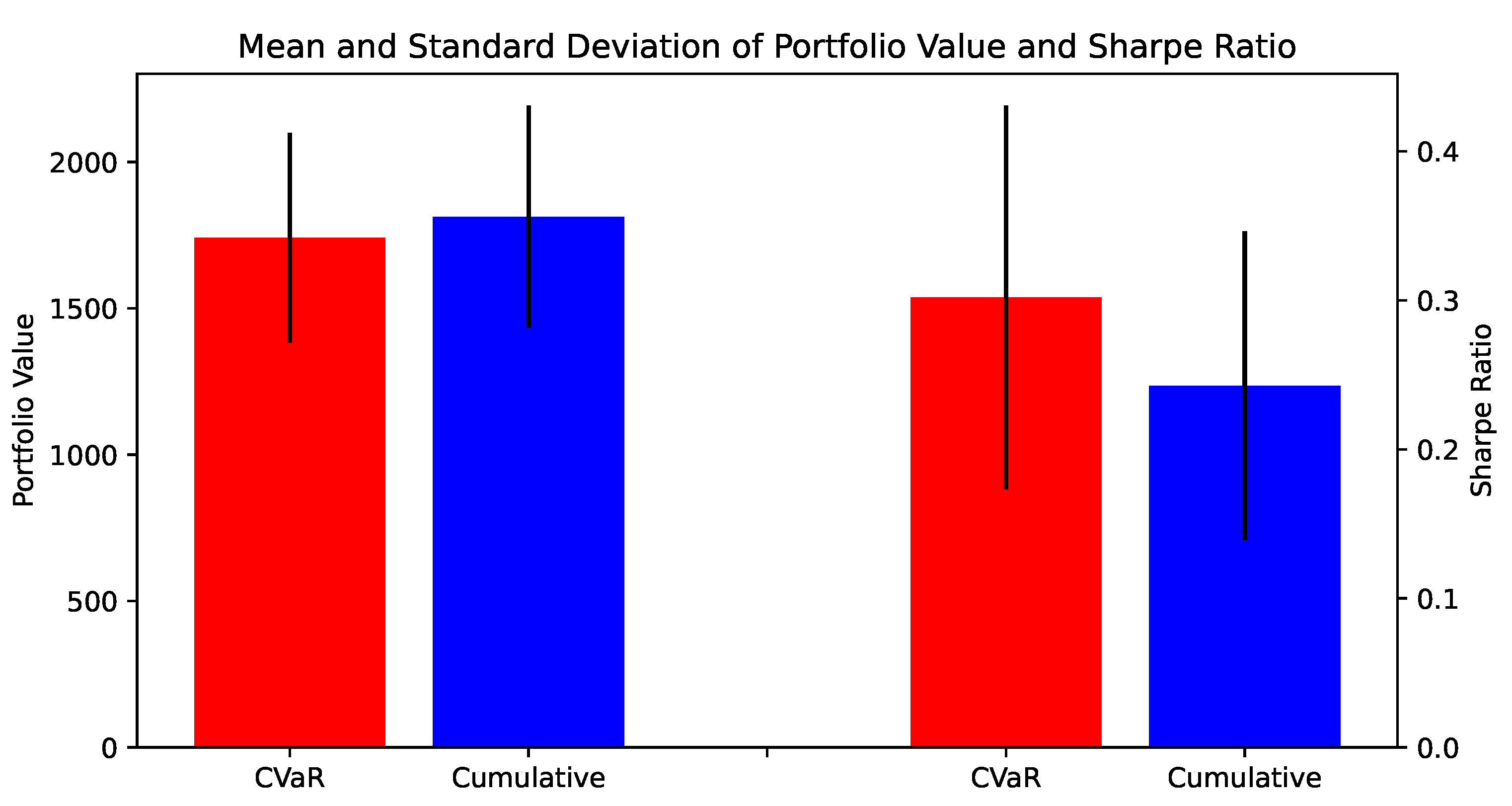
When comparing the original version, using a cumulative return for the high-level, versus the risk-return version, using CVaR as a reward, we get a significant difference, with a larger Sharpe ratio for the CVaR agent (running a t-test between the two populations, gave a p-value of 0.02, so the null hypothesis can be rejected, i.e., the two populations means are not equal).
Figure 7.
Final performance on BTCUSDT of major models tested.
Figure 7.
Final performance on BTCUSDT of major models tested.
Figure 8.
Cumulative rewards versus CVaR.
Figure 8.
Cumulative rewards versus CVaR.
To evaluate the performance of the risk-return model, we compute the monthly Sharpe ratio, which will be independent of the frequency of trading or data used. Otherwise, we risk sampling bias, with the Sharpe ratio dependent on the period length used for calculation. The
monthly Sharpe ratio is computed as follows:
where
is the average monthly excess return,
is the return of the portfolio in month
i, and
is the risk-free excess return (which can be taken to vary each month but which we keep constant for simplicity) and
n is the number of months. The risk-free return is generally quite low (initially taken as the return of US bonds); we take it as
.
5. Conclusion
Both hierarchy and prediction can improve performance significantly. Even though we haven’t seen any performance benefit from adding one-step prediction at the low-level, we have tested to see if good prediction does improve performance and ideed it is so, using true values instead of predictions does provide positive results. This means that the prediction model used for the low-level is insufficient.
For the high-level we saw that prediction used in conjunction to incrementally classifying predictions does offer significant performance improvements, even though neither of the two methods used separately offered any improvements. Moreover, we saw that changing the reward of the high-level to a risk-based measure like CVaR, transforms the whole problem into a risk-return optimization where the low-level is getting rewarded for increased returns and the high-level receives rewards for lowering the risk (or the risk measure).
6. Future directions
The current work can be extended by considering specific goals the high-level might give the low-level, like, for example, a desired (approximate) number of trades or desired amount of risk to seek for the period (Sharpe ratio or Sortino ratio). The closer to the goal, the bigger the reward for the low-level. In this way, the behaviour of the low-level agents can be constructed to specific desiderata.
One interesting behaviour which could be enacted in this type of architecture is for one agent to control the learning of the other (meta-learning), where, for example, the high-level control of a parameter with the reward of the low-level being .
Other ways the hierarchical decision-making setup can be further leveraged is to devise complementary low-level agents, where the trading dynamics is as different as possible while still retaining reasonable performance individually. Moreover, training one level of agents with some risk-measure and the other with the returns has not been explored fully in this article. For example, one could try using the risk-measure in the low-level and the returns for the high-level. Or alternatively, train them in the same time, without pretraining of the low-level. However, this is usually computationally more intensive and more unstable, adding to the usual instability of RL training.
In this article we showed how leveraging hierarchy and prediction for trading a single asset can significantly improve performance both in terms of overall returns and the Sharpe ratio. We used a much larger testing set to avoid the sampling bias usually encountered in such scenarios (cherry picking), and showed that even simple strategies like the mean reversion or moving average crossover can be leveraged with the help of an additional decision-making layer.
Furthermore, natural hierarchical structures seen in the usual portfolio management literature (e.g. asset classes, based on industry type or country) could be mapped to such a hierarchical system in a straightforward manner, providing a consistent way of dealing with heterogeneous assets.
Appendix A.
Appendix A.1. Implementation details
We use a simple trading environment with a fixed quantity size for each buy and sell (e.g.,
for BTCUSDT). We start with an initial balance of 1000USDT. We use a FIFO (first in first out) order queue, meaning that when we have multiple buys opened, we close the first one (first in) if a sell operation is requested. We do not allow selling short. We use transaction fees of
; however, recently, Bitstamp has introduced
trading fees for all coins for up to
or equivalent
5).
Because we only trade at the closing price of the hour in our simulations, the close moment of the open operation can be further optimized, and thus profits can significantly increase. We leave this for further work. The hierarchical approach can be easily extended to support another layer of decision-making at a smaller timescale.
We only take the close price (ohlcv) for the high-level model and predict the following 50 steps with DeepAR. We use the high-level model predictions in the high-level training regime such that the agent should learn when and how much to use the model if the predictions are off sometimes. One could say that this allows the RL agent to learn a policy based on the prediction model and its errors.
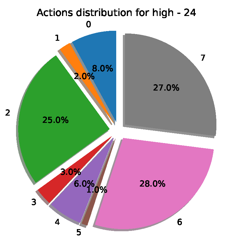
Figure A1.
Action distribution for the best HRL model.
Figure A1.
Action distribution for the best HRL model.
Appendix A.2. Hyperparameters
Table A1.
DeepAR prediction model
Table A1.
DeepAR prediction model
| Parameter |
Value |
| num_cells |
64 |
| num_layers |
2 |
| dropout_rate |
0.3 |
| prediction_length |
50 |
Table A2.
DyBM prediction model
Table A2.
DyBM prediction model
| Parameter |
Value |
| delay |
2 |
| decay |
0.9 |
| prediction_length |
1 |
| AdaGrad rate |
1.0 |
| AdaGrad delta |
1e-6 |
Table A3.
K-means clustering
Table A3.
K-means clustering
| Parameter |
Value |
| n_clusters |
5 |
| max_iter |
50 |
| metric |
euclidean |
| tolerance |
1e-6 |
Table A4.
Proximal Policy Optimization
Table A4.
Proximal Policy Optimization
| Parameter |
Value |
| use_critic |
True |
| use GAE |
True |
| GAE lambda |
1.0 |
| kl_coeff |
0.2 |
| rollout_fragment_length |
200 |
| train_batch_size |
200 |
| sgd_minibatch_size |
128 |
| shuffle_sequences |
True |
| num_sgd_iter |
30 |
| lr_schedule |
None |
| vf_loss_coeff |
1.0 |
| entropy_coeff_schedule |
grid_search([[1, 0.1], [500000, 0.0001]]) |
| clip_param |
0.3 |
| kl_target |
0.01 |
| batch_mode |
truncate_episodes |
| vf_clip_param |
grid_search([1, 10]) |
| clip_param |
grid_search([0.1, 0.2]) |
| grad_clip |
grid_search([1, 10]) |
| learning_rate_schedule |
grid_search([[[1, 1e-4], [500000, 1e-5]],
[[1, 1e-3], [500000, 1e-4]],
[[1, 1e-3], [500000, 1e-5]]]) |
| neural_network |
[1024, 512] |
References
- Mnih, V.; Kavukcuoglu, K.; Silver, D.; Rusu, A.A.; Veness, J.; Bellemare, M.G.; Graves, A.; Riedmiller, M.; Fidjeland, A.K.; Ostrovski, G.; et al. Human-level control through deep reinforcement learning. nature 2015, 518, 529–533. [Google Scholar] [CrossRef] [PubMed]
- Li, Y. Deep reinforcement learning: An overview. arXiv preprint arXiv:1701.07274 2017. arXiv:1701.07274 2017.
- Millea, A. Deep reinforcement learning for trading—A critical survey. Data 2021, 6, 119. [Google Scholar] [CrossRef]
- Pricope, T.V. Deep reinforcement learning in quantitative algorithmic trading: A review. arXiv preprint arXiv:2106.00123 2021. arXiv:2106.00123 2021.
- Zhang, Z.; Zohren, S.; Roberts, S. Deep reinforcement learning for trading. The Journal of Financial Data Science 2020, 2, 25–40. [Google Scholar] [CrossRef]
- Betancourt, C.; Chen, W.H. Deep reinforcement learning for portfolio management of markets with a dynamic number of assets. Expert Systems with Applications 2021, 164, 114002. [Google Scholar]
- Millea, A.; Edalat, A. Using Deep Reinforcement Learning with Hierarchical Risk Parity for Portfolio Optimization. International Journal of Financial Studies 2022, 11, 10. [Google Scholar]
- Ebens, H.; Kotecha, C.; Ypsilanti, A.; Reiss, A. Introducing the multi-asset strategy index. The Journal of Alternative Investments 2008, 11, 6–25. [Google Scholar] [CrossRef]
- Cornalba, F.; Disselkamp, C.; Scassola, D.; Helf, C. Multi-Objective reward generalization: Improving performance of Deep Reinforcement Learning for selected applications in stock and cryptocurrency trading. arXiv preprint arXiv:2203.04579 2022. arXiv:2203.04579 2022.
- Dai, M.; Zhang, Q.; Zhu, Q.J. Trend following trading under a regime switching model. SIAM Journal on Financial Mathematics 2010, 1, 780–810. [Google Scholar] [CrossRef]
- Ang, A.; Timmermann, A. Regime changes and financial markets. Annu. Rev. Financ. Econ. 2012, 4, 313–337. [Google Scholar]
- Sutton, R.S.; Barto, A.G. Reinforcement learning: An introduction; MIT press, 2018.
- Guo, X.; Hernández-Lerma, O. Continuous-time Markov decision processes. In Continuous-Time Markov Decision Processes; Springer, 2009; pp. 9–18.
- Yu, P.; Lee, J.S.; Kulyatin, I.; Shi, Z.; Dasgupta, S. Model-based deep reinforcement learning for dynamic portfolio optimization. arXiv preprint arXiv:1901.08740 2019. arXiv:1901.08740 2019.
- Moerland, T.M.; Broekens, J.; Jonker, C.M. Model-based reinforcement learning: A survey. arXiv preprint arXiv:2006.16712 2020. arXiv:2006.16712 2020.
- Deisenroth, M.; Rasmussen, C.E. PILCO: A model-based and data-efficient approach to policy search. In Proceedings of the Proceedings of the 28th International Conference on machine learning (ICML-11). Citeseer, 2011, pp. 465–472.
- Ha, D.; Schmidhuber, J. World models. arXiv preprint arXiv:1803.10122 2018. arXiv:1803.10122 2018.
- Wei, H.; Wang, Y.; Mangu, L.; Decker, K. Model-based reinforcement learning for predictions and control for limit order books. arXiv preprint arXiv:1910.03743 2019. arXiv:1910.03743 2019.
- Bishop, C.M. Mixture density networks. Neural Computing Research Group Report: NCRG/94/0041 1994.
- Levy, A.; Platt, R.; Saenko, K. Hierarchical actor-critic. arXiv preprint arXiv:1712.00948 2017, arXiv:1712.00948 2017, 1212. [Google Scholar]
- Nachum, O.; Gu, S.S.; Lee, H.; Levine, S. Data-efficient hierarchical reinforcement learning. Advances in neural information processing systems 2018, 31. [Google Scholar]
- Vezhnevets, A.S.; Osindero, S.; Schaul, T.; Heess, N.; Jaderberg, M.; Silver, D.; Kavukcuoglu, K. Feudal networks for hierarchical reinforcement learning. In Proceedings of the International Conference on Machine Learning. PMLR; 2017; pp. 3540–3549. [Google Scholar]
- Dietterich, T.G.; et al. The MAXQ Method for Hierarchical Reinforcement Learning. In Proceedings of the ICML. Citeseer, Vol. 98; 1998; pp. 118–126. [Google Scholar]
- Wiering, M.; Schmidhuber, J. HQ-learning. Adaptive Behavior 1997, 6, 219–246. [Google Scholar]
- Pateria, S.; Subagdja, B.; Tan, A.h.; Quek, C. Hierarchical reinforcement learning: A comprehensive survey. ACM Computing Surveys (CSUR) 2021, 54, 1–35. [Google Scholar]
- Suri, K.; Shi, X.Q.; Plataniotis, K.; Lawryshyn, Y. TradeR: Practical Deep Hierarchical Reinforcement Learning for Trade Execution. arXiv preprint arXiv:2104.00620 2021. arXiv:2104.00620 2021.
- Wang, R.; Wei, H.; An, B.; Feng, Z.; Yao, J. Commission fee is not enough: A hierarchical reinforced framework for portfolio management. arXiv preprint arXiv:2012.12620 2020. arXiv:2012.12620 2020.
- Botvinick, M.; Weinstein, A. Model-based hierarchical reinforcement learning and human action control. Philosophical Transactions of the Royal Society B: Biological Sciences 2014, 369, 20130480. [Google Scholar] [CrossRef] [PubMed]
- Xu, D.; Fekri, F. Interpretable Model-based Hierarchical Reinforcement Learning using Inductive Logic Programming. arXiv preprint arXiv:2106.11417 2021. arXiv:2106.11417 2021.
- Sutton, R.S.; Precup, D.; Singh, S. Between MDPs and semi-MDPs: A framework for temporal abstraction in reinforcement learning. Artificial intelligence 1999, 112, 181–211. [Google Scholar] [CrossRef]
- Kulkarni, T.D.; Saeedi, A.; Gautam, S.; Gershman, S.J. Deep successor reinforcement learning. arXiv preprint arXiv:1606.02396 2016. arXiv:1606.02396 2016.
- Srinivas, A.; Krishnamurthy, R.; Kumar, P.; Ravindran, B. Option discovery in hierarchical reinforcement learning using spatio-temporal clustering. arXiv preprint arXiv:1605.05359 2016. arXiv:1605.05359 2016.
- Lloyd, S. Least square quantization in PCM. Bell Telephone Laboratories Paper. Published in journal much later: Lloyd, SP: Least squares quantization in PCM. IEEE Trans. Inform. Theor.(1957/1982) 1957, 18, 11. [Google Scholar]
- Salinas, D.; Flunkert, V.; Gasthaus, J.; Januschowski, T. DeepAR: Probabilistic forecasting with autoregressive recurrent networks. International Journal of Forecasting 2020, 36, 1181–1191. [Google Scholar]
|
Disclaimer/Publisher’s Note: The statements, opinions and data contained in all publications are solely those of the individual author(s) and contributor(s) and not of MDPI and/or the editor(s). MDPI and/or the editor(s) disclaim responsibility for any injury to people or property resulting from any ideas, methods, instructions or products referred to in the content. |
© 2023 by the authors. Licensee MDPI, Basel, Switzerland. This article is an open access article distributed under the terms and conditions of the Creative Commons Attribution (CC BY) license (http://creativecommons.org/licenses/by/4.0/).
