Cosine Similarity Measures of (m, n)-Rung Orthopair Fuzzy Sets and Their Applications in Plant Leaf Diseases Classification

Preprint

Article

Cosine Similarity Measures of (m, n)-Rung Orthopair Fuzzy Sets and Their Applications in Plant Leaf Diseases Classification

Altmetrics

Downloads

147

Views

205

Comments

A peer-reviewed article of this preprint also exists.

Arpan Singh Rajput,Shailja Shukla,

Samajh Singh Thakur^*

Arpan Singh Rajput,Shailja Shukla,

Samajh Singh Thakur^*

This version is not peer-reviewed

Submitted:

22 May 2023

Posted:

23 May 2023

You are already at the latest version

Alerts

Abstract

This article introduces ten similarity measures that utilize cosine and cotangent functions to compare (m,n)-rung orthopair fuzzy sets, this a super class of q-rung orthopair fuzzy sets. Further, we applied our established weighted similarity measures to medical diagnosis, pattern recognition,and building material problems and also presented the comparison between established measures with the existing cosine and cotangent measures of q-rung orthopair, pythagorean and intuitionistic fuzzy sets. Lastly, we considered a numerical example that demonstrates the effective and scientific application of these similarity measures in plant leaf disease classification. Furthermore, we present graphical interpretations to demonstrate the effectiveness of our established measures.

Keywords:

Subject: Engineering - Electrical and Electronic Engineering

1. Introduction

The fusion of technology and generalized forms of classical sets is very useful to solve many real world complex problems which involve the vague and uncertain information. A classical set is defined by its characteristic function from universe of discourse to two point sets {0,1}.When dealing with intricate issues that encompass vague and uncertain information, classical set theory falls short. To handle the vagueness and impreciseness in complex problems, fuzzy sets (FSs) was created by Zadeh[1] as a generalization of classical sets. the application of FS theory extends to multiple fields, including control theory, artificial intelligence, pattern recognition , database system and medical diagnosis. In 1986 Atanassov[2]created intuitionistic fuzzy sets(IFS)s which is a super class of FSs. After the occurrence of Atanassov[2] paper, several generalizations of IFSs have been appeared in the literature. In the year 2013 Yager [3] presented a super class of IFSs called pythagorean fuzzy sets (PFSs). PFSs are more extensive than the IFSs and can describe more imprecise and vague information in decision making process. In 2017, Yager introduced the q-rung orthopair fuzzy sets (q-ROFSs) [4]. This innovative approach offers a highly effective and powerful tool to manage imprecise and uncertain information across a wide range of real-world applications and problems. Later in 2019, Senapati and Yager [5] developed and introduced the concept of Fermatean fuzzy sets (FFSs), which is a specific instance of q-ROFSs when q=3. Recently Ibrahim and Alshamari[6] initiated the study of (m,n-rungorthopair fuzzy sets((m,n)-ROFSs) as a super class of q-ROFSs. This concept is also independently investigated by Jun and hur[7] and AI-Shami[8] with the name of (m,n)-fuzzy sets. The (m,n)-ROFSs is more flexible and effective as compare to q-ROFSs in handling the uncertainty and vagueness in MADM and MCDM.

The similarity measure is a crucial metric that can evaluate the degree of similarity between the two objects, making it an essential tool to distinguish diverse patterns in practical applications. Researchers like Adlassnig[9], Zwick and colleagues[10], Pappis and Karacapilidis [11], Chen and colleagues [12,13], Zeng and Li[14], Mitchel[15], and others have extensively studied the similarity measures between fuzzy sets. Their research explores the potential of fuzzy sets to facilitate the development of corresponding applications in areas like image processing, medical diagnosis, pattern recognition, and decision-making. Since the emergence of interval type-2 fuzzy sets (IFSs), several similarity measures between IFSs have appeared in these literature [16,17,18,19,20,21,22,23,24,25,26,27,28,29,30]. Some researchers have investigated and studied these similarity measures between IFSs based on cosine functions, including Ye [31,35,37], Shi and Ye [32], Zhau and colleagues[36], and Liu and colleagues[38,39]. Others, such as Tian [33] and Rajarajeswari and Uma [34], have created similarity measures between IFSs based on cotangent functions and presented their applications in medical diagnosis.

PFS is a powerful tool for depicting vagueness and impreciseness in MADM and MCDM. In the recent past many researcher such as Garg [40], Zeng, Li and Qin[41],Peng, Yuan, Yang[42], Husain and Yang[43], Wei and Wei[44] and others presented different similarity measures between PFSs for solving MADM problems. Recently different similarity measures between FFSs and their applications in MADM and MCDM have been appeared in the literature [45,46,47,48,49]. The q-ROFSs is a powerful mathematical tool for handling uncertain, imprecise, and vague information in real-world problems, surpassing PFS and FFS in terms of capability. In 2019, Peng and Dai[51] introduced a similarity measure between q-ROFSs that assessed the quality of classroom teaching. Jan and his colleagues[52] considered the generalized dice similarity between ROFSs. Farhadinia and his team explored a range of similarity measures for q-ROFSs. Peng and Liu[54] investigated information measures for q-ROFSs. Additionally, Liu, Chen, and Peng[55] as well as Wang and his team[56] introduced several similarity measures between q-ROFSs based on cosine and cotangent functions and explored their properties and applications. The (m,n)-ROFSs through double universes are more flexible and efficient than the m-ROFS and n-ROFS in discussing the symmetry between multiple objects. In other words, (m,n)-ROFSs are capable of more effectively addressing MADM problems, including all q-ROFS decision-making problems as a special case.

The structure of this article is as follows. In section two, a review is presented on generalized fuzzy structures along with their cosine and cotangent similarity measures. Section three is devoted to establishing similarity measures and weighted similarity measures between (m,n)-ROFSs based on cosine and cotangent functions. Section four compares the newly established similarity measures for (m,n)-ROFSs with existing measures for q-ROFSs, PFSs, and IFSs based on cosine and cotangent functions. The comparison is made by considering pattern recognition, medical diagnosis, and building material problems discussed in the literature. In section five, the established similarity measures are utilized in the classification of plant leaf disease, and the effectiveness and reasonableness of the proposed measures are demonstrated. Finally, section six concludes in the article with some closing remarks.

2. Preliminaries

In this section, we will examine different types of generalized fuzzy structures and the cosine and cotangent similarity measures that are currently in use for these structures. For the remainder of the paper, we assume that

P

is a finite, discrete, and non-empty discourse set consisting of r elements, denoted as

p_{1}, p_{2}, . . ., p_{r}

3. Preliminaries

P

is a finite, discrete, and non-empty discourse set consisting of r elements, denoted as

p_{1}, p_{2}, . . ., p_{r}

3.1. Generalized Fuzzy Structures

Definition 1.

Let consider this,

P

be a fixed set. A structure

E = {〈 p, ϑ_{E} (p), ς_{E} (p) 〉 : p \in P}

where,

ϑ_{E} : P \to [0, 1]

and

ς_{E} : P \to [0, 1]

denotes the membership (written as MF) and non-membership function (written as NMF) of

E

, is called :

(a): Intuitionistic fuzzy set (written as IFS) [2] in $P$ if $0 \leq ϑ_{E} (p) + ς_{E} (p) \leq 1$ , $\forall$ $p \in P$ .
(b): Pythagorean fuzzy set (written as PFS)[3] in $P$ if $0 \leq {(ϑ_{E} (p))}^{2} + {(ς_{E} (p))}^{2} \leq 1$ , $\forall$ $p \in P$ .
(c): Fermatean fuzzy set (written as FFS)[5] in $P$ if $0 \leq {(ϑ_{E} (p))}^{3} + {(ς_{E} (p))}^{3} \leq 1$ , $\forall$ $p \in P$ .
(d): q-ROFSs [4] in $P$ if $0 \leq {(ϑ_{E} (p))}^{q} + {(ς_{E} (p))}^{q} \leq 1$ , $\forall$ $p \in P$ and $q \in N$ .

Definition 2.

[6,7,8] A (m,n)-rung orthopair fuzzy set (written as (m,n)-ROFSs)

E

in an universe of discourse

P

is a structure

\begin{matrix} E = {〈 p, (ϑ_{E} (p), ς_{E} (p)) 〉 : p \in P} \end{matrix}

where

ϑ_{E} : P \to [0, 1]

and

ς_{E} : P \to [0, 1]

denotes the MF and NMF of

E

which satisfies the condition

\begin{matrix} 0 \leq {(ϑ_{E} (p))}^{m} + {(ς_{E} (p))}^{n} \leq 1 \end{matrix}

∀ p

\in P

and m, n

\in N

Remark 1.

[6,7,8] A (m,n)-ROFSs

E

P

coincides with IFS (resp. PFSs , FFSs, q-ROFSs ) if m,n=1,1 ( resp. m,n=2,2, m,n=3,3, m,n=q,q).

The family of all (m,n)-ROFSs defined over

P

will be referred by

(m, n) - R O F S s (P)

Definition 3.

[6,7,8] For any (m,n)-ROFSs

E = {〈 p, ϑ_{E} (p), ς_{E} (p) 〉 : p \in P}

E_{1} = {〈 p, ϑ_{E_{1}} (p), ς_{E_{1}} (p) 〉 : p \in P}

and

E_{2} = {〈 p, ϑ_{E_{2}} (p), ς_{E_{2}} (p) 〉 : p \in P}

P

The subset, equality, union, intersection and complement operations over

(m, n) - R O F S (X)

are defined as follow:

(a): $E_{1} ⋐ E_{2} \Leftrightarrow ϑ_{E_{1}} (p) \leq ϑ_{E_{2}} (p)$ and $ς_{E_{1}} (p) \geq ς_{E_{2}} (p)$ $\forall p \in P$ ;
(b): $E_{1} = E_{2} \Leftrightarrow ϑ_{E_{1}} = ϑ_{E_{2}}$ and $ς_{E_{1}} = ς_{E_{2}}$ ;
(c): $E_{1} ⋓ E_{2} = \{\begin{matrix} 〈 p, ϑ_{E_{1}} (p) ⋁ ϑ_{E_{2}} (p), \\ ς_{E_{1}} (p) ⋀ ς_{E_{2}} (p) 〉 : p \in P \end{matrix}\}$ ;
(d): $E_{1} ⋒ E_{2} = \{\begin{matrix} 〈 p, ϑ_{E_{1}} (p) ⋀ ϑ_{E_{2}} (p), \\ ς_{E_{1}} (p) ⋁ ς_{E_{2}} (p) 〉 : p \in P \end{matrix}\}$ ;
(e): $E^{c} = {〈 p, {(ς_{E} (p))}^{\frac{n}{m}}, {(ϑ_{E} (p))}^{\frac{m}{n}} : p \in P}$ .

Proposition 1.

[6,7,8] Let

E_{1} = {〈 p, ϑ_{E_{1}} (p), ς_{E_{1}} (p) 〉 : p \in P}

and

E_{2} = {〈 p, ϑ_{E_{2}} (p), ς_{E_{2}} (p) 〉 : p \in P}

be two (m,n)-ROFSs on

P

. Then:

(a): $E_{1} ⋓ E_{2} = E_{2} ⋓ E_{1}$ .
(b): $E_{1} ⋒ E_{2} = E_{2} ⋒ E_{1}$ .
(c): ${(E_{1}^{c})}^{c} = E_{1}$ .
(d): ${(E_{1} ⋓ E_{2})}^{c} = E_{1}^{c} ⋒ E_{2}^{c}$ .
(e): ${(P_{1} ⋒ E_{2})}^{c} = E_{1}^{c} ⋓ E_{2}^{c}$ .

Definition 4.

For each (m,n)-ROFSs

E

P

, the degree of indeterminacy membership(written as IMD)

π_{E}

(p) can be expressed as

\begin{matrix} π_{E} (p) = \sqrt[\frac{m + n}{2}]{{(1 - ϑ_{E} (p))}^{m} + {(ς_{E} (p))}^{n}} \end{matrix}

\forall p \in P

Remark 2.

The IDM

π_{E} (p)

p \in P

to IFS(resp. PFSs, FFSs,q-ROFSs)

E

is a special case of IDM

π_{E} (p)

of p to (m,n)-ROFSs

E

for m=n=1 (resp. m,n=2,2, m,n=3,3, m,n=q,q).

Remark 3.

Clearly, for each (m,n)-ROFS

E

P

\begin{matrix} π_{E}^{\frac{m + n}{2}} (p) + {(ϑ_{E} (p))}^{m} + {(ς_{E} (p))}^{n} = 1 \end{matrix}

\forall p \in P

3.2. Cosine and Cotangent Similarity Measures for Generalized Fuzzy Structures

For the calculation of the degree of proximity between any two objects used the cosine and cotangent similarity measures, which have been applied in numerus MADM and MCDM methods. The study of cosine measure between two IFSs

E

and

F

are iniatiated by Ye[31] in 2011. In 2013 Shi and Ye[32]created new cosine similarity measures for IFSs which are the extension of the measures proposed by Ye [31] and applied in fault diagnosis of Turbine. In 2016 Ye[35] created two cosine similarity measures for IFSs based on cosine functions and applied them in MADM. The Cotangent function based similarity measures for IFSs was created by Tian[33] and Rajeshwari and Uma [34] in 2013. The weighted cosine and cotangent similarity measures between IFSs are defined by Ye[31], Shi and Ye[32], Tian[33] and Rajarajeshwari and Uma[34]. In 2018 Wei and wei[44] proposed cosine and cotangent measures between two PFSs

E

{〈 p_{j}, ϑ_{E} (p_{j}), ς_{E} (p_{j}) 〉 : p_{j} \in P}

and

F

{〈 p_{j}, ϑ_{F} (p_{j}), ς_{F} (p_{j}) 〉 : p_{j} \in P}

over

P = {p_{j} : j = 1, 2, . . r}

which are shown in Table 1.

The weighted cosine and cotangent measures between two PFSs

E

and

F

for weighted vector

{[ω_{1}, ω_{2}, . . . ω_{n}]}^{T}

satisfying the condition

Σ_{j = 1}^{j = r} ω_{j} = 1

are also proposed by Wei and wei[44] which are shown in Table 2.

In 2019 Wang and his coworkers [56] extended cosine and cotangent measures of similarity for q-ROFSs which are shown in Table 3 and Table 4. The cosine and cotangent similarity and weighted similarity measures for IFSs and PFSs are the special cases of corresponding similarity measures defined by Wang and his coworkers [56]. Recently Kirisci [48] created some cosine similarity measures for Fermatean fuzzy sets which is a special case of q-ROFSs for q=3.

4. Cosine and Cotangent Similarity Measures for (m,n)-ROFSs

The (m,n)-ROFSs described by the degree of membership and non-membership, for which sum of m-th power of membership degree and n-th power of non-membership degree is lies between 0 and 1,is more general than the IFSs , PFSs and q-ROFSs and can describe more vague and imprecise information. In other words, the (m,n)-ROFSs can deal with the MADM and MCDM problems which IFSs, PFSs and q-ROFSs cannot and it is clear that IFSs, PFSs, and q-ROFSs are the special the (m,n)-ROFSs, which indicates (m,n)-ROFSs can be more effective and powerful tool to deal with vagueness and impreciseness involved in MADM and MCDM problems. In this section we shall propose the (m,n)-rung orthopair fuzzy cosine similarity measures and (m,n)-rung orthopair fuzzy cotangent similarity measures under (m,n)-ROFSs environment which are new extensions of the similarity measures of IFSs, PFSs and q-ROFSs.

4.1. Cosine similarity measures for (m,n)-ROFSs

In this section, a cosine similarity measure and a weighted cosine similarity measure with (m,n)-ROFSs information are created in an analogous manner to the cosine similarity measure and weighted cosine similarity measure for IFSs, PFSs and q-ROFSs.

Definition 5.

Let

P = {p_{1}, p_{2}, . . . p_{r}}

be a fixed set. Assume

E

{〈 p_{j}, ϑ_{E} (p_{j}), ς_{E} (p_{j}) 〉 | p_{j} \in P}

and

F

{〈 p_{j}, ϑ_{F} (p_{j}), ς_{F} (p_{j}) 〉 | p_{j} \in P}

be two (m,n)-ROFSs of

P

. Then the (m,n)-ROFSs cosine measure

(m, n) - R O F C^{1}

between

E

and

F

is defined as:

(m, n) - R O F C^{1} (E, F) =

\frac{1}{r} \sum_{j = 1}^{r} \frac{ϑ_{E}^{m} (p_{j}) ϑ_{F}^{m} (p_{j}) + ς_{E}^{n} (p_{j}) ς_{F}^{n} (p_{j})}{\sqrt{{(ϑ_{E}^{m} (p_{j}))}^{2} + {(ς_{E}^{n} (p_{j}))}^{2}} \sqrt{{(ϑ_{F}^{m} (p_{j}))}^{2} + {(ς_{F}^{n} (p_{j}))}^{2}}}

(1)

Remark 4.

The cosine measures

I F C^{1} (E, F)

(resp.

P F C^{1} (E, F)

q - R O F C^{1} (E, F)

) for IFSs (resp. PFSs, q-ROFSs) are the special cases of cosine similarity measures of

(m, n) - R O F C^{1} (E, F)

of (m,n)-ROFSs for m,n=1,1 (resp. m,n=2,2; m,n=q,q).

Proposition 2.

Let

P = {p_{1}, p_{2}, . . . p_{r}}

and

E, F \in (m, n) - R O F S (P)

. Then the cosine similarity measure of

(m, n) - R O F C^{1} (E, F)

satisfies the following conditions:

(i): $0 \leq (m, n) - R O F C^{1} (E, F) \leq 1$ .
(ii): $(m, n) - R O F C^{1} (E, F) = (m, n) - R O F C^{1} (F, E)$ .
(iii): $E = F \Rightarrow (m, n) - R O F C^{1} (E, F)$ = 1.

Proof.

The proofs of (i) and (ii) are obvious.

(iii) If

E = F

. Then

ϑ_{E} (p_{j}) = ϑ_{F} (p_{j})

and

ς_{E} (p_{j}) = ς_{F} (p_{j})

for j= 1,2,⋯ n. Thus from Equation (1) we obtain that

(m, n) - R O F C^{1} (E, F)

= 1 □

Proposition 3.

Let

P = {p_{1}, p_{2}, . . . p_{r}}

and

E, F \in (m, n) - R O F S (P)

. Then the distance measure of angle defined as

\begin{matrix} d (E, F) = a r c c o s ((m, n) - R O F C^{1} (E, F)) \end{matrix}

Meets the specified conditions:

(i): d( $E, F$ ) ≥ 0,
(ii): $E = F \Rightarrow d (E, F)$ =0.
(iii): $d (E, F) = d (F, E)$ .
(iv): $d (E, G) \leq d (E, F) + d (F, G)$ if $E ⋐ F ⋐ G$ for any $G \in (m, n) - R O F S (P)$ .

Proof.

Proofs of conditions (i),(ii) and (iii) follows from Proposition2. (iv) Suppose that

E \subseteq F \subseteq G

for any (m.n)-ROFS

G = {〈 p_{j}, ϑ_{T} (p_{j}), ς_{T} (p_{j}) 〉 | p_{j} \in P}

over

P

. Since Equation (1) is a sum of terms, it is appropriate to examine the distance measures based on the angle between the vectors:

d_{j} (E (p_{j}), F (p_{j}))

= a r c c o s ((m, n) - R O F C_{j}^{1} (E (p_{j}), F (p_{j})))

d_{j} (E (p_{j}), G (p_{j}))

= a r c c o s ((m, n) - R O F C_{j}^{1} (E (p_{j}), G (p_{j})))

d_{j} (F (p_{j}), G (p_{j})) = a r c c o s ((m, n) - R O F C_{j}^{1} (F (p_{j}), G (p_{j})))

(j = 1, 2, \dots r)

. Where,

(m, n) - R O F C_{j}^{1} (E (p_{j}), F (p_{j})

= \frac{ϑ_{E}^{m} (p_{j}) ϑ_{F}^{m} (p_{j}) + ς_{E}^{n} (p_{j}) ς_{F}^{n} (p_{j})}{\sqrt{{(ϑ_{E}^{m} (p_{j}))}^{2} + {(ς_{E}^{n} (p_{j}))}^{2}} \sqrt{{(ϑ_{F}^{m} (p_{j}))}^{2} + {(ς_{F}^{n} (p_{j}))}^{2}}}

(m, n) - R O F C_{j}^{1} (E (p_{j}), G (p_{j})

= \frac{ϑ_{E}^{m} (p_{j}) ϑ_{G}^{m} (p_{j}) + ς_{E}^{n} (p_{j}) ς_{G}^{n} (p_{j})}{\sqrt{{(ϑ_{E}^{m} (p_{j}))}^{2} + {(ς_{E}^{n} (p_{j}))}^{2}} \sqrt{{(ϑ_{G}^{m} (p_{j}))}^{2} + {(ς_{G}^{n} (p_{j}))}^{2}}}

(m, n) - R O F C_{j}^{1} (F (p_{j}), G (p_{j})

= \frac{ϑ_{F}^{m} (p_{j}) ϑ_{G}^{m} (p_{j}) + ς_{F}^{n} (p_{j}) ς_{G}^{n} (p_{j})}{\sqrt{{(ϑ_{F}^{m} (p_{j}))}^{2} + {(ς_{F}^{n} (p_{j}))}^{2}} \sqrt{{(ϑ_{G}^{m} (p_{j}))}^{2} + {(ς_{G}^{n} (p_{j}))}^{2}}}

For three vectors

E (p_{j}) = 〈 ϑ_{E} (p_{j}), ς_{E} (p_{j}) 〉

F (p_{j}) = 〈 ϑ_{F} (p_{j}), ς_{F} (p_{j}) 〉

G (p_{j}) = 〈 ϑ_{G} (p_{j})

ς_{G} (p_{j}) 〉

in one plane, if the

E (p_{j}) \subseteq F (p_{j}) \subseteq G (p_{j})

j = 1, 2, \dots

,r. Then by triangle inequality we get that

d_{j} (E (p_{j}), G (p_{j})) \leq d_{j} (E (p_{j}), F (p_{j})) + d_{j} (F (p_{j}), G (p_{j}))

. Combining the inequality with Equation (1), we can get

d (E, G) \leq d (E, F) + d (F, G)

. Hence the distance measure of angle d(

E, F

) satisfies the property (iv). □

Now we define (m,n)-ROFSs cosine measure by considering three terms membership degree(written as MD), non-membership degree(written as NMD), and indeterminacy membership(written as IMD) of (m,n)-ROFSs.

Definition 6.

Let

E

{〈 p_{j}, ϑ_{E} (p_{j}), ς_{E} (p_{j}) 〉 | p_{j} \in P}

and

F

{〈 p_{j}, ϑ_{F} (p_{j}), ς_{F} (p_{j}) 〉 | p_{j} \in P}

be two (m,n)-ROFSs in

P

. Then (m,n)-rung orthopair fuzzy cosine measure (

(m, n) - R O F C^{2}

) between

E

and

F

can be expressed as:

(m, n) - R O F C^{2} (E, F)

\frac{1}{r} \sum_{j = 1}^{r} \frac{(\begin{matrix} ϑ_{E}^{m} (p_{j}) ϑ_{F}^{m} (p_{j}) + ς_{E}^{n} (p_{j}) ς_{F}^{n} (p_{j}) + π_{E}^{\frac{m + n}{2}} (p_{j}) π_{F}^{\frac{m + n}{2}} (p_{j}) \end{matrix})}{(\begin{matrix} (\sqrt{{(ϑ_{E}^{m} (p_{j}))}^{2} + {(ς_{E}^{n} (p_{j}))}^{2} + {(π_{E}^{\frac{m + n}{2}} (p_{j}))}^{2}}) (\sqrt{{(ϑ_{F}^{m} (p_{j}))}^{2} + {(ς_{F}^{n} (p_{j}))}^{2} + {(π_{F}^{\frac{m + n}{2}} (p_{j}))}^{2}}) \end{matrix})}

(2)

Proposition 4.

Consider two (m,n)-ROFSs, denoted by

E

and

F

, defined over

P

. Then the cosine similarity measure

(m, n) - R O F C^{2} (E, F)

satisfies the following conditions:

(i): $0 \leq (m, n) - R O F C^{2} (E, F) \leq 1$ .
(ii): $(m, n) - R O F C^{2} (E, F) = (m, n) - R O F C^{2} (F, E)$ .
(iii): $E = F \Rightarrow (m, n) - R O F C^{2} (E, F)$ =1.

Remark 5.

The cosine measures

I F C^{2} (E, F)

(resp.

P F C^{2} (E, F)

q - R O F C^{2} (E, F)

) for IFSs (resp. PFSs, q-ROFSs) are the special cases of cosine similarity measures

(m, n) - R O F C^{2} (E, F)

of (m,n)-ROFSs for m,n=1,1 (resp. m,n=2,2; m,n=q,q).

Now we define the (m,n)-ROFSs weighted cosine measures between two (m,n)-ROFSs

E

and

F

by Considering the weighting vector of the elements in (m,n)-ROFSs.

Definition 7.

Let

P = {p_{1}, p_{2}, . . . p_{r}}

be a fixed set and

E, F \in (m, n) - R O F S (P)

. Assume

ω

{(ω_{1}, ω_{2}, \dots, ω_{n})}^{T}

, be the weighting vector of the elements

p_{j}

(j = 1, 2, ⋯ ,r) satisfies the condition

\sum_{j = 1}^{r} ω_{j} = 1

, ∀

ω_{j}

∈ [0, 1] and j = 1, 2, ⋯, r . Then the (m,n)-rung orthopair fuzzy weighted cosine measures

(m, n) - R O F W C^{1}

and

(m, n) - R O F W C^{2}

between

E

and

F

can be expressed as :

(m, n) - R O F W C^{1} (E, F)

\sum_{j = 1}^{r} ω_{j} \frac{(\begin{matrix} ϑ_{E}^{m} (p_{j}) ϑ_{F}^{m} (p_{j}) + ς_{E}^{n} (p_{j}) ς_{F}^{n} (p_{j}) \end{matrix})}{(\begin{matrix} (\sqrt{{(ϑ_{E}^{m} (p_{j}))}^{2} + {(ς_{E}^{n} (p_{j}))}^{2}}) (\sqrt{{(ϑ_{F}^{m} (p_{j}))}^{2} + {(ς_{F}^{n} (p_{j}))}^{2}}) \end{matrix})}

(3)

(m, n) - R O F W C^{2} (E, F)

\sum_{j = 1}^{r} ω_{j} \frac{(\begin{matrix} ϑ_{E}^{m} (p_{j}) ϑ_{F}^{m} (p_{j}) + ς_{E}^{n} (p_{j}) ς_{F}^{n} (p_{j}) + π_{E}^{\frac{m + n}{2}} (p_{j}) π_{F}^{\frac{m + n}{2}} (p_{j}) \end{matrix})}{(\begin{matrix} (\sqrt{{(ϑ_{E}^{m} (p_{j}))}^{2} + {(ς_{E}^{n} (p_{j}))}^{2} + {(π_{E}^{\frac{m + n}{2}} (p_{j}))}^{2}}) (\sqrt{{(ϑ_{F}^{m} (p_{j}))}^{2} + {(ς_{F}^{n} (p_{j}))}^{2} + {(π_{F}^{\frac{m + n}{2}} (p_{j}))}^{2}}) \end{matrix})}

(4)

When we take the weighting vector

ω

{(\frac{1}{r}, \frac{1}{r}, \dots, \frac{1}{r})}^{T}

, then the weighted cosine similarity measures

(m, n) - R O F W C^{1} (E, F)

and

(m, n) - R O F W C^{2} (E, F)

will reduce to cosine similarity measures

(m, n) - R O F C^{1} (E, F)

and

(m, n) - R O F C^{2} (E, F)

respectively.

Remark 6.

The weighted cosine similarity measures

W I F C^{k} (E, F)

(resp.

W P F C^{k} (E, F)

q - R O F W C^{k} (E, F)

) for IFSs (resp. PFSs, q-ROFSs) are the special cases of weighted cosine similarity measures

(m, n) - R O F W C^{k} (E, F)

(k=1,2) of (m,n)-ROFSs for m,n=1,1 (resp. m,n=2,2; m,n=q,q).

Example 1.

Let

P = {p_{1}, p_{2}, p_{3}}

and

\begin{matrix} E = {(p_{1}, 0.5, 0.8), (p_{2}, 0.6, 0.4), (p_{3}, 0.8, 0.3)} \\ F = {(p_{1}, 0.7, 0.6), (p_{2}, 0.8, 0.2), (p_{3}, 0.4, 0.3)} \end{matrix}

be two (m,n)-ROFSs over

P

. Assume m = 4, n=3 and

ω = {(0.20, 0.45, 0.35)}^{T}

be a weighting vector of the elements

p_{1}, p_{2}, p_{3}

. Then

(m, n) - R O F W C^{1} (E, F)

= 0.8150899 and

(m, n) - R O F W C^{2} (E, F)

= 0.8610532.

Proposition 5.

Let

E

and

F

be two (m,n)-ROFSs over a fixed set

P = {p_{1}, p_{2}, . . . p_{r}}

. Assume

ω

{(ω_{1}, ω_{2}, \dots, ω_{n})}^{T}

, be the weighting vector of the elements

p_{j}

(j = 1, 2, ⋯ ,r) satisfies the condition

\sum_{j = 1}^{r} ω_{j} = 1

, ∀

ω_{j}

∈ [0, 1] and j = 1, 2, ⋯, r. Then the weighted cosine similarity measures

(m, n) - R O F W C^{k} (E, F)

(k=1,2) meets the following conditions.

(a): $0 \leq (m, n) - R O F W C^{k} (E, F) \leq 1$ .
(b): $(m, n) - R O F W C^{k} (E, F) = (m, n) - R O F W C^{k} (F, E)$ .
(c): $E = F \Rightarrow (m, n) - R O F W C^{k} (E, F)$ =1.

4.2. Similarity Measures of (m,n)-ROFSs Based on Cosine Function

This section introduces several (m,n)-ROFSs cosine similarity measures between (m,n)-ROFSs, which are based on cosine function, and explores their properties.

Definition 8.

Let

P = {p_{j} : j = 1, 2, . . . r}

and

\begin{matrix} E = {〈 p_{j}, (ϑ_{E} (p_{j}), ς_{E} (p_{j})) 〉 | p_{j} \in P} \\ F = {〈 p_{j}, (ϑ_{F} (p_{j}), ς_{F} (p_{j})) 〉 | p_{j} \in P} \end{matrix}

be two (m,n)-ROFSs over

P

. Then two (m,n)-ROFSs cosine similarity measures

(m, n) - R O F C S^{k}

(k=1,2) between

E

and

F

can be expressed as:

(m, n) - R O F C S^{1} (E, F)

\frac{1}{r} \sum_{j = 1}^{r} c o s [\frac{π}{2} (\begin{matrix} | ϑ_{E}^{m} (p_{j}) - ϑ_{F}^{m} (p_{j}) | \lor | ς_{E}^{n} (p_{j}) - ς_{F}^{n} (p_{j}) | \end{matrix})]

(5)

(m, n) - R O F C S^{2} (E, F)

\frac{1}{r} \sum_{j = 1}^{r} c o s [\frac{π}{4} (\begin{matrix} | ϑ_{E}^{m} (p_{j}) - ϑ_{F}^{m} (p_{j}) | + | ς_{E}^{n} (p_{j}) - ς_{F}^{n} (p_{j}) | \end{matrix})]

(6)

Proposition 6.

Let

P = {p_{1}, p_{2}, \dots, p_{r}}

and

E, F \in (m, n) - R O F S (P)

. Then the (m,n)-rung orthopair fuzzy cosine similarity measures

(m, n) - R O F C S^{k} (E, F)

(k = 1, 2) meets the following properties:

(a): $0 \leq (m, n) - R O F C S^{k} (E, F) \leq 1$ .
(b): $(m, n) - R O F C S^{k} (E, F) = 1 \Leftrightarrow E = F$ .
(c): $(m, n) - R O F C S^{k} (E, F)$ $= (m, n) - R O F C S^{k} (F, E)$ .
(d): If $E \subseteq F \subseteq G$ , $\forall G \in (m, n) - R O F S (P)$ . Then $(m, n) - R O F C S^{k} (E, G) \leq (m, n) - R O F C S^{k} (E, F)$ and $(m, n) - R O F C S^{k} (E, G) \leq (m, n) - R O F C S^{k} (F, G)$ .

Proof. (a) The values of cosine functions lie between 0 and 1, which makes it evident.

(b) If

E = F

foe any two (m,n)-ROFSs

E

and

F

P = {p_{1}, p_{2}, \dots, p_{r}}

. Then for each j=1,2,⋯,r,

ϑ_{E}^{m} (p_{j}) = ϑ_{F}^{m} (p_{j})

and

ς_{E}^{n} (p_{j}) = ς_{F}^{n} (p_{j})

. It implies that |

ϑ_{E}^{m} (p_{j}) - ϑ_{F}^{m} (p_{j})

| = 0 and |

ς_{E}^{n} (p_{j}) - ς_{F}^{n} (p_{j})

| = 0. Hence

(m, n) - R O F C S^{k} (E, F)

=1 for k=1,2. Suppose

(m, n) - R O F C S^{k} (E, F)

=1,k=1,2. Then |

ϑ_{E}^{m} (p_{j}) - ϑ_{F}^{m} (p_{j})

| =0 and |

ς_{E}^{n} (p_{j}) - ς_{F}^{n} (p_{j})

| = 0, for all j=1,2,⋯,r. Since cos(0) =1, there are

ϑ_{E}^{m} (p_{j}) = ϑ_{F}^{m} (p_{j})

ς_{E}^{n} (p_{j}) = ς_{F}^{n} (p_{j})

(j=1,2,⋯,r). Hence

E = F

(c)Obvious.

(d) If

E (p_{j}) \subseteq F (p_{j}) \subseteq G (p_{j})

, ∀ j=1,2,⋯,r. Then

ϑ_{E} (p_{j}) \leq ϑ_{F} (p_{j}) \leq ϑ_{G} (p_{j})

and

ς_{E} (p_{j}) \geq ς_{F} (p_{j}) \geq ς_{G} (p_{j})

, j=1,2,⋯,r. It follows that

ϑ_{E}^{m} (p_{j}) \leq ϑ_{F}^{m} (p_{j}) \leq ϑ_{G}^{m} (p_{j})

and

ς_{E}^{n} (p_{j}) \geq ς_{F}^{n} (p_{j}) \geq ς_{G}^{n} (p_{j})

. Thus we obtain that,

ϑ_{E}^{m} (p_{j}) - ϑ_{F}^{m} (p_{j})

|≤|

ϑ_{E}^{m} (p_{j}) - ϑ_{G}^{m} (p_{j})

| ,

ϑ_{F}^{m} (p_{j}) - ϑ_{G}^{m} (p_{j})

|≤|

ϑ_{E}^{m} (p_{j}) - ϑ_{G}^{m} (p_{j})

ς_{E}^{n} (p_{j}) - ς_{F}^{n} (p_{j})

|≤|

ς_{E}^{n} (p_{j}) - ς_{G}^{n} (p_{j})

| ,

ς_{F}^{n} (p_{j}) - ς_{G}^{n} (p_{j})

|≤|

ς_{E}^{n} (p_{j}) - ς_{G}^{n} (p_{j})

□

The fact that the cosine function is a decreasing function with the interval [0,

\frac{π}{2}

], therefor we obtain that

(m, n) - R O F C S^{k} (E, G) \leq (m, n) - R O F C S^{k} (E, F)

(m, n) - R O F C S^{k} (E, G) \leq (m, n) - R O F C S^{k} (F, G)

for k =1,2.

Next, we introduce (m,n)-rung orthopair fuzzy cosine measures based on cosine function. These measures are obtained by considering MD, NMD, and IMD for two (m,n)-ROFSs

E

and

F

P

Definition 9.

Let

P = {p_{j} : j = 1, 2, . . . r}

and

\begin{matrix} E = {〈 p_{j}, (ϑ_{E} (p_{j}), ς_{E} (p_{j})) 〉 | p_{j} \in P} \\ F = {〈 p_{j}, (ϑ_{F} (p_{j}), ς_{F} (p_{j})) 〉 | p_{j} \in P} \end{matrix}

be the two (m,n)-ROFSs over

P

. Then two (m,n)-ROFSs cosine similarity measures

(m, n) - R O F C S^{k})

(k=3,4) between

E

and

F

by considering MD, NMD and IMD can be expressed as:

(m, n) - R O F C S^{3} (E, F)

\frac{1}{r} \sum_{j = 1}^{r} c o s [\frac{π}{2} (\begin{matrix} | ϑ_{E}^{m} (p_{j}) - ϑ_{F}^{m} (p_{j}) |, \lor | ς_{E}^{n} (p_{j}) - ς_{F}^{n} (p_{j}) |, \lor | π_{E}^{\frac{m + n}{2}} (p_{j}) - | π_{F}^{\frac{m + n}{2}} (p_{j}) | \end{matrix})]

(7)

(m, n) - R O F C S^{4} (E, F)

\frac{1}{r} \sum_{j = 1}^{r} c o s [\frac{π}{4} (\begin{matrix} | ϑ_{E}^{m} (p_{j}) - ϑ_{F}^{m} (p_{j}) | + | ς_{E}^{n} (p_{j}) - ς_{F}^{n} (p_{j}) | + | π_{E}^{\frac{m + n}{2}} (p_{j}) - | π_{F}^{\frac{m + n}{2}} (p_{j}) | \end{matrix})]

(8)

Remark 7.

The cosine measures

I F C S^{k} (E, F)

(resp.

P F C S^{k} (E, F)

q - R O F W C S^{k} (E, F)

) for IFSs (resp. PFSs, q-ROFSs) are the special cases of cosine measures

(m, n) - R O F C S^{k} (E, F)

(k=1,2,3,4) of (m,n)-ROFSs for m,n=1,1 (resp. m,n=2,2; m,n=q,q).

We will now introduce the (m,n)-ROFSs weighted cosine measures between two (m,n)-ROFSs, which are based on cosine functions.

E

and

F

by taking into account the weighting vector associated with the elements in (m,n)-ROFSs.

Definition 10.

Let

E

{〈 p_{j}, ϑ_{E} (p_{j}), ς_{E} (p_{j}) 〉 | p_{j} \in P}

and

F

{〈 p_{j}, ϑ_{F} (p_{j}), ς_{F} (p_{j}) 〉 | p_{j} \in P}

be two (m,n)-ROFSs in

P

and ω =

{(ω_{1}, ω_{2}, \dots, ω_{r})}^{T}

be the weighting vector of the elements

p_{j}

(j = 1, 2, ⋯ , r) satisfies the condition

\sum_{j = 1}^{r} ω = 1

, ∀

ω_{j}

∈ [0, 1] and j = 1, 2, ⋯, r. Then the (m,n)-ROFSs weighted cosine measures

(m, n) - R O F W C S^{k}

, (k=1,2,3,4) between

E

and

F

on bases of cosine functions can be represented as :

(m, n) - R O F W C S^{1} (E, F)

\frac{1}{r} \sum_{j = 1}^{r} ω_{j} c o s [\frac{π}{2} (\begin{matrix} | ϑ_{E}^{m} (p_{j}) - ϑ_{F}^{m} (p_{j}) | \lor | ς_{E}^{n} (p_{j}) - ς_{F}^{n} (p_{j}) | \end{matrix})]

(9)

(m, n) - R O F W C S^{2} (E, F)

\frac{1}{r} \sum_{j = 1}^{r} ω_{j} c o s [\frac{π}{4} (\begin{matrix} | ϑ_{E}^{m} (p_{j}) - ϑ_{F}^{m} (p_{j}) | + | ς_{E}^{n} (p_{j}) - ς_{F}^{n} (p_{j}) | \end{matrix})]

(10)

(m, n) - - R O F W C S^{3}

(

E, F

) =

\frac{1}{r} \sum_{j = 1}^{r} ω_{j} c o s [\frac{π}{2} (\begin{matrix} | ϑ_{E}^{m} (p_{j}) - ϑ_{F}^{m} (p_{j}) | \lor | ς_{E}^{n} (p_{j}) - ς_{F}^{n} (p_{j}) | \lor | π_{E}^{\frac{m + n}{2}} (p_{j}) - π_{F}^{\frac{m + n}{2}} (p_{j}) | \end{matrix})]

(11)

(m, n) - R O F W C S^{4} (E, F)

\frac{1}{r} \sum_{j = 1}^{r} ω_{j} c o s [\frac{π}{4} (\begin{matrix} | ϑ_{E}^{m} (p_{j}) - ϑ_{F}^{m} (p_{j}) | + | ς_{E}^{n} (p_{j}) - ς_{F}^{n} (p_{j}) | + | π_{E}^{\frac{m + n}{2}} (p_{j}) - π_{F}^{\frac{m + n}{2}} (p_{j}) | \end{matrix})]

(12)

When the weighting vector

ω_{j} = \frac{1}{r}

j = 1, 2, \dots r

, then for k=1,2,3,4 we have (m,n)- ROFWCS

^{k} (E, F)

= (m,n)-ROFCS

^{k} (E, F)

Remark 8.

The weighted cosine similarity measures

W I F C S^{k} (E, F)

(resp.

W P F C S^{k} (E, F)

q - R O F W C S^{k} (E, F)

) for IFSs (resp. PFSs, q-ROFSs) are the special cases of weighted cosine measures

(m, n) - R O F W C S^{k} (E, F)

(k=1,2,3,4) of (m,n)-ROFSs for m,n=1,1 (resp. m,n=2,2; m,n=q,q).

Example 2.

Let

P = {p_{1}, p_{2}, p_{3}}

and

\begin{matrix} E = {(p_{1}, 0.8, 0.5), (p_{2}, 0.4, 0.6), (p_{3}, 0.3, 0.8)} \\ F = {(p_{1}, 0.6, 0.7), (p_{2}, 0.2, 0.8), (p_{3}, 0.4, 0.3)} \end{matrix}

be two (m,n)-ROFSs over

P

. Assume m = 4, n=6 and

ω = {(0.25, 0.55, 0.20)}^{T}

be the weights for the elements

p_{1}, p_{2}, p_{3}

. Then:

\begin{matrix} (m, n) - R O F W C S^{1} (E, F) = 0.928372534 . \\ (m, n) - R O F W C S^{2} (E, F) = 0.974350944 . \\ (m, n) - R O F W C S^{3} (E, F) = 0.928372534 . \\ (m, n) - R O F W C S^{4} (E, F) = 0.928372534 . \end{matrix}

Proposition 7.

Assume that there are any two (m,n)-ROFSs

E

and

F

P = {p_{1}, p_{2}, \dots, p_{r}}

, the (m,n)-ROFSs weighted cosine similarity measures (m,n)-

R O F W C S^{k}

(

E, F

)(k = 1, 2,3,4) should satisfy the properties (a)–(b):

(a): $0 \leq (m, n) - R O F W C S^{k} (E, F) \leq 1$ .
(b): $(m, n) - R O F W C S^{k} (E, F) = 1 \Leftrightarrow E = F$ .
(c): $(m, n) - R O F W C S^{k} (E, F)$

$= (m, n) - R O F W C S^{k} (F, E)$ .
(d): If $E \subseteq F \subseteq G$ , $\forall G \in (m, n) - R O F S (P)$ . Then (m,n)-ROFWCS $^{k}$ $(E, G)$ ≤(m,n)-ROFWCS $^{k}$ $(E, F)$ , (m,n)-ROFWCS $^{k}$ $(E, G)$ ≤ (m,n)-ROFWCS $^{k}$ $(F, G)$ .

4.3. Cotangent Based Similarity Measures for (m,n)-ROFSs

Definition 11.

Let

P = {p_{1}, p_{2}, . . . p_{r}}

and

E

{〈 p_{j}, (ϑ_{E} (p_{j}), ς_{E} (p_{j})) 〉 | p_{j} \in P}

F

{〈 p_{j}, (ϑ_{F} (p_{j}), ς_{F} (p_{j})) 〉 | p_{j} \in P}

be two (m,n)-ROFSs. Then (m,n)-ROFSs cotangent measures

(m, n) - R O F C o t^{1}

and

(m, n) - R O F C o t^{2}

between

E

and

F

are defined as follows:

(m, n) - R O F C o t^{1} (E, F)

\frac{1}{r} \sum_{j = 1}^{r} c o t [\frac{π}{4} + \frac{π}{4} (\begin{matrix} | ϑ_{E}^{m} (p_{j}) - ϑ_{F}^{m} (p_{j}) | \lor | ς_{E}^{n} (p_{j}) - ς_{F}^{n} (p_{j}) | \end{matrix})]

(13)

(m, n) - R O F C o t^{2} (E, F)

\frac{1}{r} \sum_{j = 1}^{r} c o t [\frac{π}{4} + \frac{π}{8} (\begin{matrix} | ϑ_{E}^{m} (p_{j}) - ϑ_{F}^{m} (p_{j}) | + | ς_{E}^{n} (p_{j}) - ς_{F}^{n} (p_{j}) | \end{matrix})]

(14)

We will now incorporate the MD, NMD and IMD - all of which are components of (m,n)-ROFSs - to define two additional cotangent similarity measures between two (m,n)-ROFSs.

Definition 12.

Let

P = {p_{j} : j = 1, 2, \dots, r}

and

\begin{matrix} E = {〈 p_{j}, (ϑ_{E} (p_{j}), ς_{E} (p_{j}) 〉 : p_{j} \in P} F = {〈 p_{j}, (ϑ_{F} (p_{j}), ς_{F} (p_{j})) 〉 : p_{j} \in P} \end{matrix}

. be two (m,n)-ROFSs in

P

. Then the (m,n)-ROFSs cotangent similarity measures

(m, n) - R O F C o t^{3}

and

(m, n) - R O F C o t^{4}

between

E

and

F

can be expressed as:

(m, n) - R O F C o t^{3} (E, F)

\frac{1}{r} \sum_{j = 1}^{r} c o t [\frac{π}{4} + \frac{π}{4} (\begin{matrix} | ϑ_{E}^{m} (p_{j}) - ϑ_{F}^{m} (p_{j}) | \lor | ς_{E}^{n} (p_{j}) - ς_{F}^{n} (p_{j}) | \lor | π_{E}^{\frac{m + n}{2}} (p_{j}) - π_{F}^{\frac{m + n}{2}} (p_{j}) | \end{matrix})]

(15)

(m, n) - R O F C o t^{4}

(

E, F

) =

\frac{1}{r} \sum_{j = 1}^{r} c o t [\frac{π}{4} + \frac{π}{8} (\begin{matrix} | ϑ_{E}^{m} (p_{j}) - ϑ_{F}^{m} (p_{j}) | + | ς_{E}^{n} (p_{j}) - ς_{F}^{n} (p_{j}) | + | π_{E}^{\frac{m + n}{2}} (p_{j}) - π_{F}^{\frac{m + n}{2}} (p_{j}) | \end{matrix})]

(16)

Remark 9.

The cotangent measures

I F C T^{k} (E, F)

(resp.

P F C T^{k} (E, F)

q - R O F C o t^{k} (E, F)

) for IFSs (resp. PFSs, q-ROFSs) are the special cases of cotangent measures

(m, n) - R O F C o t^{k} (E, F)

(k=1,2,3,4) of (m,n)-ROFSs for m,n=1,1 (resp. m,n=2,2; m,n=q,q).

We will now introduce the (m,n)-ROFSs weighted cotangent measures between two (m,n)-ROFSs

E

and

F

by taking into account the weighting vector associated with the elements in (m,n)-ROFSs.

Definition 13.

Let

P = {p_{1}, p_{2}, . . . p_{r}}

be a fixed set and

E

{〈 p_{j}, ϑ_{E} (p_{j}), ς_{E} (p_{j}) 〉 | p_{j} \in P}

F

{〈 p_{j}, ϑ_{F} (p_{j}), ς_{F} (p_{j}) 〉 | p_{j} \in P}

be two (m,n)-ROFSs in

P

. Assume ω =

{(ω_{1}, ω_{2}, \dots, ω_{r})}^{T}

be the weighting vector of the elements

p_{j}

(j = 1, 2, ⋯ , r) satisfies the condition

\sum_{j = 1}^{r} ω_{j} = 1

, ∀

ω_{j}

∈ [0,1] and j = 1, 2, ⋯, r.

Then the (m,n)-ROFSs weighted cotangent measures

(m, n) - R O F W C o t^{k}

(k=1,2,3,4) between

E

and

F

are expressed as follows:

(m, n) - R O F W C o t^{1} (E, F)

\sum_{j = 1}^{r} ω_{j} c o t [\frac{π}{4} + \frac{π}{4} (\begin{matrix} | ϑ_{E}^{m} (p_{j}) - ϑ_{F}^{m} (p_{j}) | \lor | ς_{E}^{n} (p_{j}) - ς_{F}^{n} (p_{j}) | \end{matrix})]

(17)

(m, n) - R O F W C o t^{2} (E, F)

\sum_{j = 1}^{r} ω_{j} c o t [\frac{π}{4} + \frac{π}{8} (\begin{matrix} | ϑ_{E}^{m} (p_{j}) - ϑ_{F}^{m} (p_{j}) | + | ς_{E}^{n} (p_{j}) - ς_{F}^{n} (p_{j}) | \end{matrix})]

(18)

(m, n) - R O F W C o t^{3} (E, F)

\sum_{j = 1}^{r} ω_{j} c o t [\frac{π}{4} + \frac{π}{4} (\begin{matrix} | ϑ_{E}^{m} (p_{j}) - ϑ_{F}^{m} (p_{j}) | \lor | ς_{E}^{n} (p_{j}) - ς_{F}^{n} (p_{j}) | \lor | π_{E}^{\frac{m + n}{2}} (p_{j}) - π_{F}^{\frac{m + n}{2}} (p_{j}) | \end{matrix})]

(19)

(m, n) - R O F W C o t^{4} (E, F)

\sum_{j = 1}^{r} ω_{j} c o t [\frac{π}{4} + \frac{π}{8} (\begin{matrix} | ϑ_{E}^{m} (p_{j}) - ϑ_{F}^{m} (p_{j}) | + | ς_{E}^{n} (p_{j}) - ς_{F}^{n} (p_{j}) | + | π_{E}^{\frac{m + n}{2}} (p_{j}) - π_{F}^{\frac{m + n}{2}} (p_{j}) | \end{matrix})]

(20)

When we let weighting vector

ω

{(\frac{1}{r}, \frac{1}{r}, \dots \frac{1}{r})}^{T}

, then

(m, n) - R O F W C o t^{k} (E, F)

coincides with

(m, n) - R O F C o t^{k} (E, F)

, for k=1,2,3,4.

Example 3.

Let

X = {p_{1}, p_{2}, p_{3}}

and

\begin{matrix} E = {(p_{1}, 0.4, 0.9), (p_{2}, 0.9, 0.3), (p_{3}, 0.9, 0.6)} \\ F = {(p_{1}, 0.3, 0.7), (p_{2}, 0.8, 0.3), (p_{3}, 0.7, 0.4)} \end{matrix}

be two (m,n)-ROFSs over

P

. Assume m = 5, n=7 and

ω_{1}

= 0.25,

ω_{2}

= 0.35 and

ω_{1}

=0.40 be the weights for the elements

p_{1}, p_{2}, p_{3}

.Then:

\begin{matrix} (m, n) - R O F W C o t^{1} (E, F) = 0.529085874 . \\ (m, n) - R O F W C o t^{2} (E, F) = 0.720632612 . \\ (m, n) - R O F W C o t^{3} (E, F) = 0.525336422 . \\ (m, n) - R O F W C o t^{4} (E, F) = 0.525336422 . \end{matrix}

Remark 10.

The weighted cotangent similarity measures

W I F C T^{k} (E, F)

(resp.

W P F C T^{k} (E, F)

q - R O F W C o t^{k} (E, F)

) for IFSs (resp. PFSs, q-ROFSs) are the special cases of weighted cotangent measures

(m, n) - R O F W C o t^{k} (E, F)

(k=1,2,3,4) of (m,n)-ROFSs for m,n=1,1 (resp. m,n=2,2; m,n=q,q).

5. Comparisons of Existing Similarity Measures and Proposed Similarity Measures

In this section, a comparison is made between the existing cosine and cotangent similarity measures for IFSs, PFSs, and q-ROFSs, and the newly established cosine and cotangent similarity measures for (m,n)-ROFSs. This comparison is based on the pattern recognition and medical diagnosis examples of Wei and Wei[44], as well as the building material classification example of Wang and his colleagues[56].

Example 4.

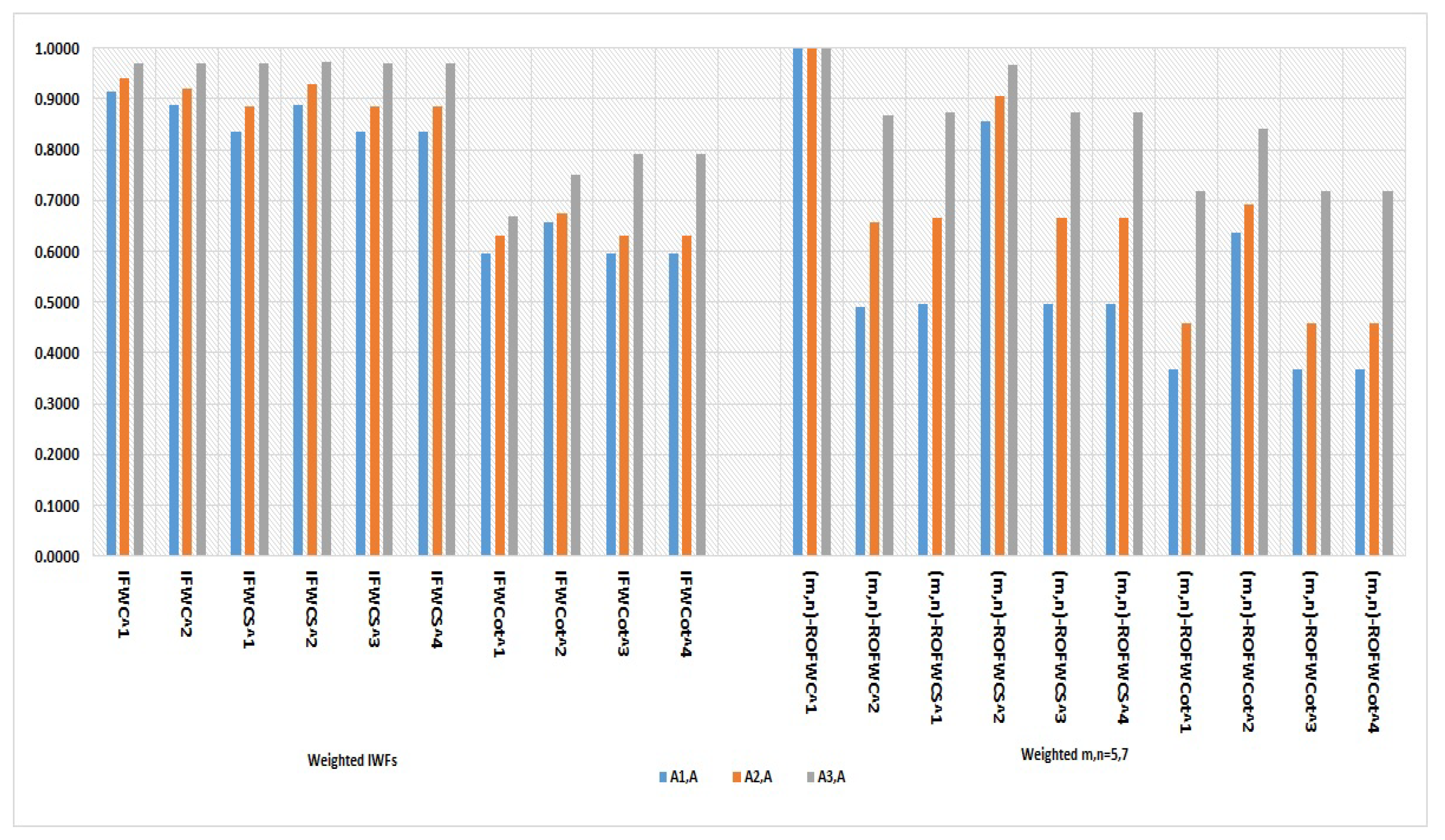
let’s take the example of [44]and the relevant data is presented in Table 5 in which suppose we have three known patterns

E_{i}

(i=1,2,3), represented by IFSs

E_{i}

(i=1,2,3) in the feature space

P = {p_{1}, p_{2}, p_{3}}

. We also have an unknown pattern

E

that needs to be recognized. The weight are considered as

w = {(0.5, 0.3, 0.2)}^{T}

For the given pattern recognition, example for IFSs, Table 6 shows the results of weighted WIFSs obtained by the wei et. al [44] and Table 7 shows the proposed weighted cosine and cotangent similarity measures (m,n)-ROFWSs for

m = 5

and

n = 7,

with similar weighted values of

0.5,

0.3,

and

0.2,

, respectively. Where, it is clearly visible that for all ten weighted similarity measures,

(E_{3}, E)

has the largest value, indicating that the unknown pattern

E

is most similar to

E_{3} .

Suggesting that the unknown pattern M is most similar to

E_{3}

Example 5.

Consider[44] a set of symptoms

S = {s_{1}, s_{2}, s_{3}, s_{4}, s_{5}}

, where

s_{1}

corresponds to Temperature,

s_{2}

to Headache,

s_{3}

to Stomach Pain,

s_{4}

to Cough, and

s_{5}

to Chest Pain. Let

D_{1}

(Viral Fever),

D_{2}

(Malaria),

D_{3}

(Typhoid),

D_{4}

(Stomach Problem), and

D_{5}

(Chest Problem) be the five possible diagnoses represented by

(m, n) - R O F S s

, as shown in Table 8. The weights

w = {(0.15, 0.25, 0.20, 0.15, 0.25)}^{T}

are assigned to the symptoms.

Figure 1. Comparison graph between weighted WIFSs and the proposed weighted (m,n)-ROFWSs. In this figure it is evident that the value in weighted WIFSs and proposed weighted (m,n)-ROFWSs for

m, n = 5, 7

show that

E_{3}

has the largest and most consistent value. This indicates that the unknown pattern

E

is most similar to

E_{3}

Figure 1. Comparison graph between weighted WIFSs and the proposed weighted (m,n)-ROFWSs. In this figure it is evident that the value in weighted WIFSs and proposed weighted (m,n)-ROFWSs for

m, n = 5, 7

show that

E_{3}

has the largest and most consistent value. This indicates that the unknown pattern

E

is most similar to

E_{3}

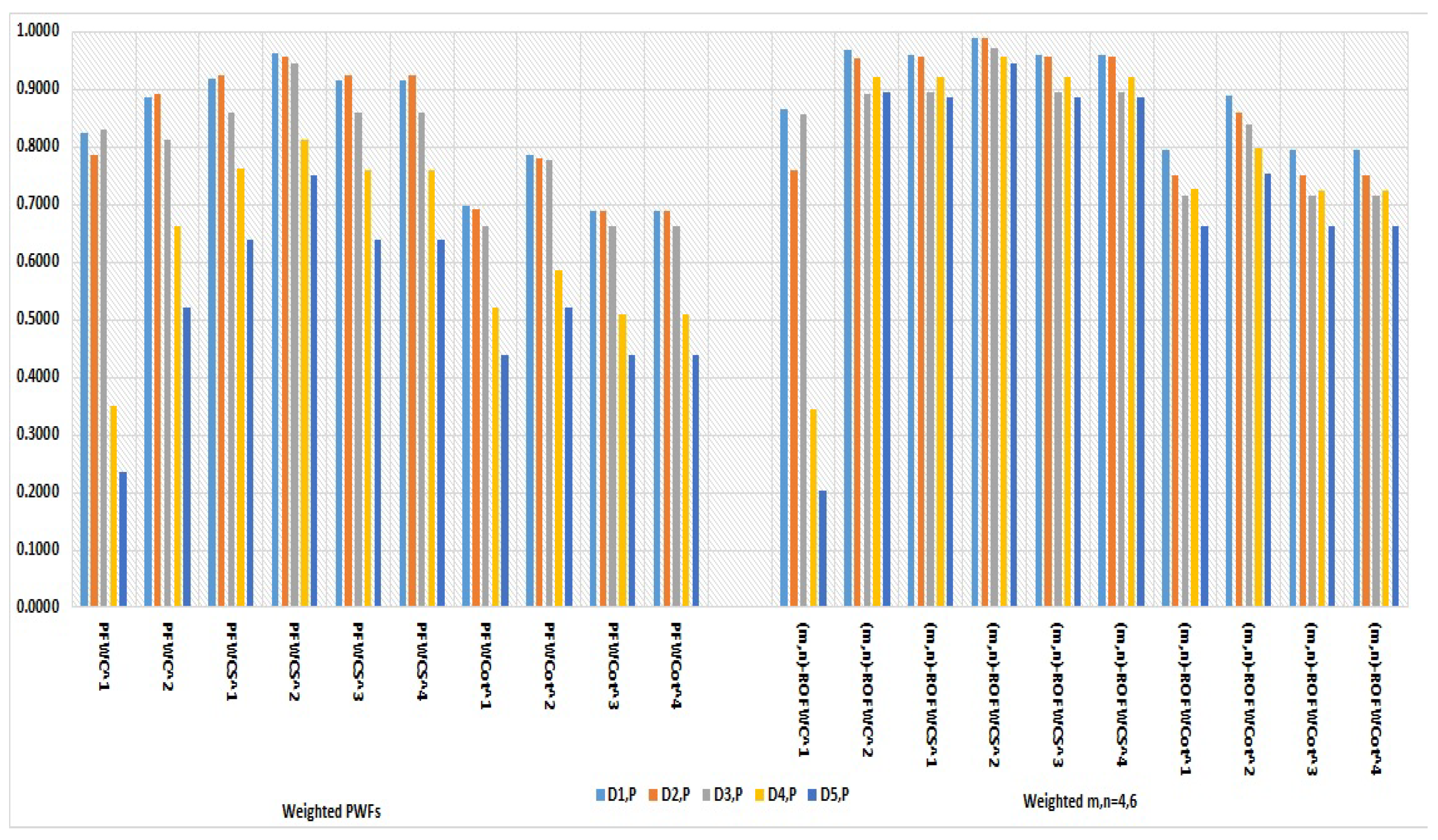
In this medical example containing all values of pythagorean fuzzy sets, Table 9 shows the results obtained using ten weighted pythagorean similarity measures (WPFSs). The calculated results reveal inconsistencies in

(D_{3}, E)

(D_{2}, E)

, and

(D_{1}, E)

, making it difficult to accurately diagnose the disease. Therefore, a specific disease should be considered.

Table 10 displays the results obtained using the proposed

(m, n) - R O F W S s

method with

m = 4

and

n = 6

. These results demonstrate that all ten weighted similarity measures identify patient

D

with disease

D_{1}

, with the highest degree of weighted similarity between

E

and

D_{1}

. These findings suggest that the proposed method is reliable and accurate in diagnosing the patient’s disease.

Upon comparing the results presented in Table 9 and Table 10, it becomes evident that the proposed weighted

(m, n) - R O F W S s

method is more accurate than the method proposed by Wei et al. [44] in assigning Disease to the consistent class

(D_{1}, E)

. Therefore, our proposed method is more reliable and accurate.

Figure 2. Comparison graph between weighted WPFSs and the proposed weighted (m,n)-ROWFSs. In this Figure it is evident that the WPFSs values in Table 9 are inconsistent and proposed weighted (m,n)-ROFWSs for

m, n = 4, 6

show that

D_{1}

has the largest and most consistent values. This indicates that the Patient

E

is having the disease to

D_{1}

which viral fever.

m, n = 4, 6

show that

D_{1}

has the largest and most consistent values. This indicates that the Patient

E

is having the disease to

D_{1}

which viral fever.

Example 6.

Let us consider[56] a scenario where there are five known building construction materials, represented by q-ROFSs

Z_{i}

(i=1,2,3,4,5), in the feature space

P = {p_{1}, p_{2}, p_{3}, p_{4}, p_{5}}

, as shown in Table 11. We also have an unknown building material

Z

that needs to be classified into one of the following classes:

Z_{1}

Z_{2}

Z_{3}

Z_{4}

Z_{5}

. Assuming that the weights w =( 0.15, 0.20,0.25,0.10,0.30)

^{T}

, we aim to determine the degree of similarity between

Z_{3}

and

E

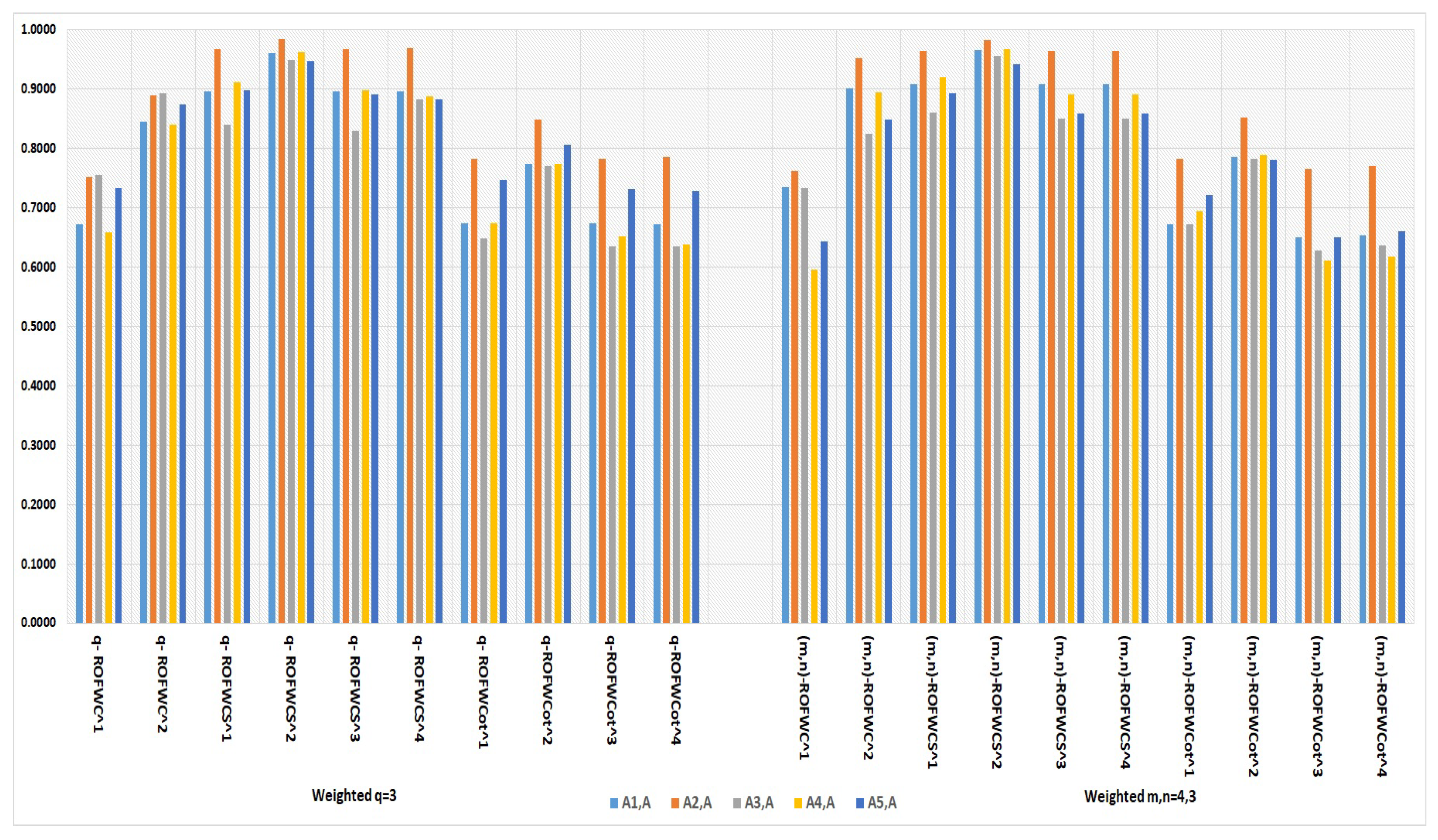
the results represented in Table 12 indicate that, degree of weighted similarity between

Z_{3}

and

E

is the largest among the ten weighted similarity measures, for all building materials except

q - R O F W C^{1}

. Therefore, based on the principle of maximum weighted The q-ROFSs smililarity, the ten similarity measures can define the unknown building material

E

as being similar to the known building material

E_{2}

Table 13 shows the results obtained by the proposed weighted similarity measures

(m, n) - R O F W S s

for

m = 4

and

n = 3

. Based on these results, it is evident in table [13] that all ten similarity measures allocate unknown building material

E

to building material

E_{2}

, with the degree of weighted similarity between

E

and

E_{2}

being the largest. This suggests that the proposed weighted

(m, n) - R O F W S s

method is accurate in allocating unknown building materials to known building materials.

By comparing the results presented in Table 12 and Table 13, it is clear that the proposed weighted

(m, n) - R O F W S s

method is more accurate than the method proposed by P. Wang et al. [56] for assigning unknown building materials to the consistent class (

E_{2}

E

). Therefore,our results are more reliable and accurate.

Figure 3. Comparison graph between weighted q-ROFWSs and proposed weighted (m,n)-ROWFSs. In this figure it is represented that, the value of weighted q-ROFWSs for all building materials except for

q - R O F W C^{1}

, the degree of weighted similarity between (

E_{3}

E

) is the largest among in ten weighted similarity measures and proposed weighted (m,n)-ROFWSs for

m = 4, n = 3

show that

E_{3}

has the largest and most consistent value. This indicates that the unknown pattern

E

is most similar to

E_{3}

q - R O F W C^{1}

, the degree of weighted similarity between (

E_{3}

E

) is the largest among in ten weighted similarity measures and proposed weighted (m,n)-ROFWSs for

m = 4, n = 3

show that

E_{3}

has the largest and most consistent value. This indicates that the unknown pattern

E

is most similar to

E_{3}

6. Applications of Proposed Similarity Measures in the Classification of Plant Leaf Disease

Plants are an integral component of our ecosystem that provides us with vital resources such as oxygen and food. However, these crucial organisms are vulnerable to various diseases that can have a significant impact on their growth and survival. One of the most prevalent problems that plants face is leaf disease, which can result in a considerable reduction in crop yield and quality, significantly affecting farmers livelihoods and the economy as a whole. This article aims to explore the issue of plant leaf disease and the measures that can be taken to prevent and manage it. Plant leaf diseases can be caused by several factors, such as bacteria, fungi, viruses, and other pathogens. Common types of leaf diseases include powdery mildew, downy mildew, leaf spot, and rust. These diseases can affect various parts of plants, including leaves, stems, and fruits, leading to discoloration, distortion, and wilting. In severe cases, the leaves may fall off, leading to stunted growth and reduced yield. Several factors can facilitate the spread of plant leaf diseases, such as high humidity, poor air circulation, and contaminated soil or water. Additionally, using infected planting materials and inadequate crop management practices can also contribute to the spread of these diseases.

plant leaf diseases pose a significant problem that can adversely affect crop yield and quality, ultimately impacting the livelihoods of farmers and the economy. Preventing and managing these diseases require a combination of preventive and curative measures, including the use of disease-resistant plant varieties, good agricultural practices, and judicious use of chemical treatments. By taking these measures, we can ensure that our plants remain healthy and continue to provide us with the essential resources we need for our survival.

Tomato plants are susceptible to various leaf diseases that can negatively impact their growth and yield. Preventing these diseases can be achieved through various methods, including planting disease-resistant tomato varieties, keeping the soil well-drained, and avoiding overhead watering. Additionally, it is important to remove any infected plant parts and keep the garden clean to prevent the spread of disease.

In the next example we proposed the method to classify the plant leaf disease using proposed cosine and cotangent similarity and weighted similarity measures.

Example 7.

Let us consider, a set of five symptoms

q = {q_{1}, q_{2}, q_{3}, q_{4}, q_{5}}

where

q_{1}

= Dark brown leaf,

q_{2}

= Brown Leaf,

q_{3}

= Yellow leaf,

q_{4}

= Patches,

q_{5}

= spots and a set of five diagnosis

Z_{i} (i = 1, 2, 3, 4, 5)

, which are presented by (m,n)-ROFSs,

Z_{1}

(Gray leaf spot),

Z_{2}

(Bacterial Canker),

Z_{3}

(Bacterial Speck),

Z_{4}

(Bacterial Spot),

Z_{5}

(Early Blight) defined in Table 14 and Consider a sample pattern

Z

that will be recognized.

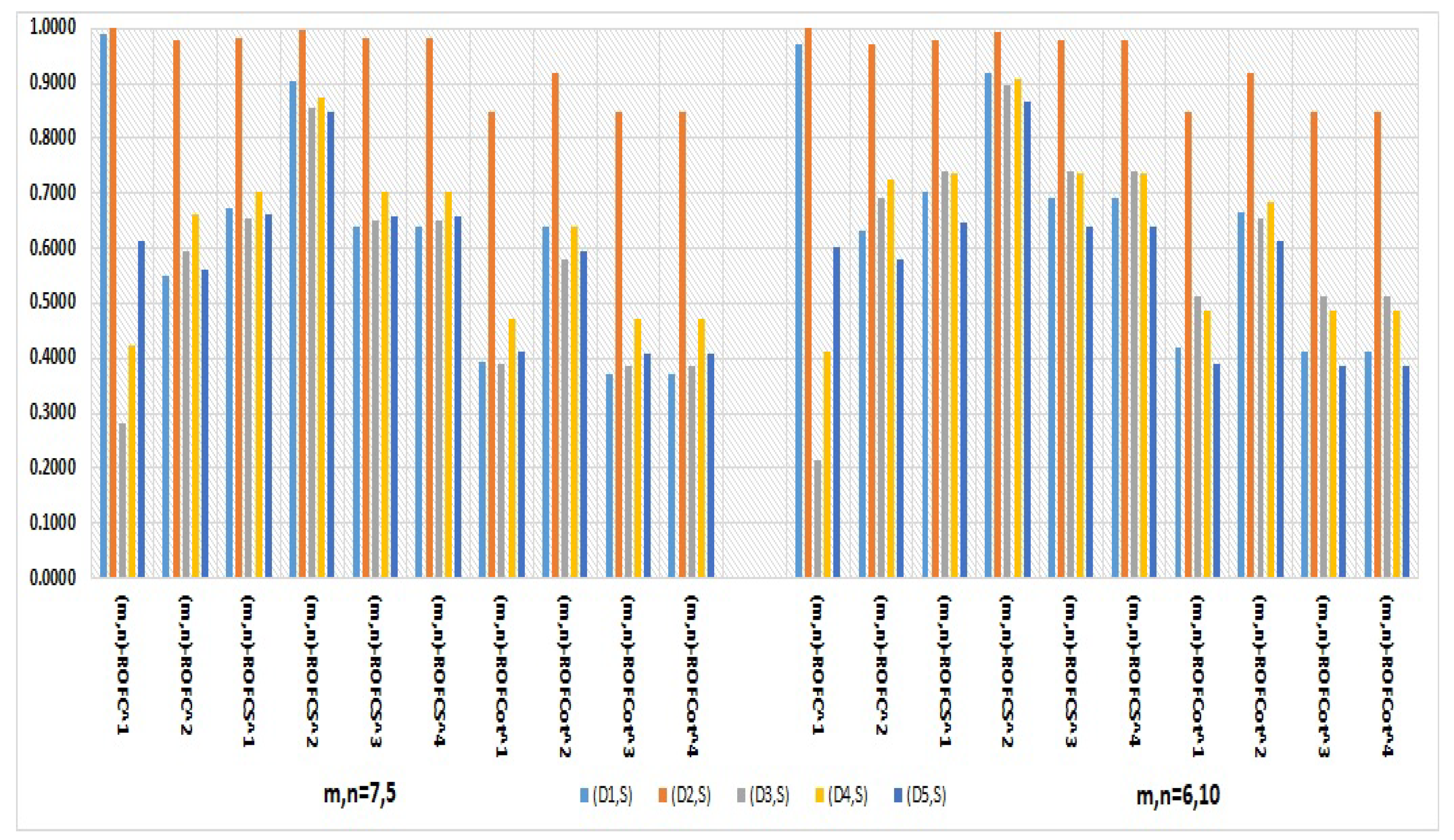
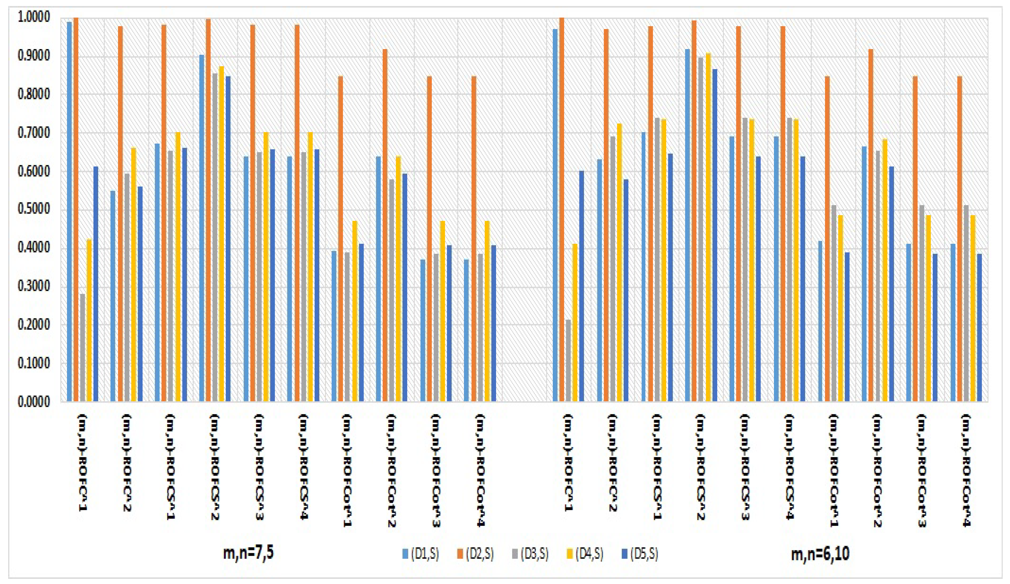
For the given plant leaf disease application,the proposed cosine and cotangent similarity measures for

(m, n) - R O F S s

for the values m=5,n=7 and m=6,n=10 are shown in Table 15 and Table 16. The similarity measures for m=7,n=5 and m=6,n=10 values respectively shows consistent and accurate results, indicating that all ten proposed similarity measures also shows

Z_{2}

as having the largest value, suggesting that the sample

Z

is most similar to

Z_{2}

Figure 4. Results of proposed (m,n)-ROFSs for two Different values of m and n. This figure represents a graph for ten similarity measures of (m,n)-ROWFs for different

m, n = 5, 7

and

m, n = 6, 10

, which shows that

Z_{2}

has the largest value. This suggests that the sample

Z

is most similar to the disease category of

Z_{2}

Figure 4. Results of proposed (m,n)-ROFSs for two Different values of m and n. This figure represents a graph for ten similarity measures of (m,n)-ROWFs for different

m, n = 5, 7

and

m, n = 6, 10

, which shows that

Z_{2}

has the largest value. This suggests that the sample

Z

is most similar to the disease category of

Z_{2}

If we consider the weights of

w = (0.10, 0.30, 0.25,

{0.15, 0.20)}^{T}

. The proposed weighted cosine and cotangent similarity measures (m, n)-ROFWSs for

m = 7

n = 5

,and

m = 6

n = 10

are presented in Table 17 and Table 18 respectively. The accurate and consistent results indicate that all ten proposed weighted similarity measures also shows

Z_{2}

as having the largest value, suggesting that the sample

Z

is most similar to

Z_{2}

Figure 5. Results of proposed weighted (m,n)-ROFWSs for two different values of m and n. this Figure represents a graph for ten weighted similarity measures of (m,n)-ROWFs for different

m, n = 5, 7

and

m, n = 6, 10

, which shows that

Z_{2}

has the largest value. This suggests that the sample

Z

is most similar to the disease category of

Z_{2}

Figure 5. Results of proposed weighted (m,n)-ROFWSs for two different values of m and n. this Figure represents a graph for ten weighted similarity measures of (m,n)-ROWFs for different

m, n = 5, 7

and

m, n = 6, 10

, which shows that

Z_{2}

has the largest value. This suggests that the sample

Z

is most similar to the disease category of

Z_{2}

7. Discussion

By comparing all the results shown in Table 15, Table 16, Table 17 and Table 18 it is clear that for four different conditions of m and n, we get the most accurate and consistent result, from which we can easily classify the sample disease leaf

Z

as belonging to Disease

Z_{2}

which is Bacterial canker.

Remark 11.

The cosine similarity measures proposed by Ye[31,35] and Shi, Ye[32] and cotangent similarity measures for IFSs proposed by Tian[33], Rajeshwari and Uma [34] can not classified the plant leaf disease for (m,n)-rung ortho pair fuzzy information which is not a intuitionistic fuzzy information given in Table 14.

Remark 12.

The cosine and cotangent similarity and weighted similarity measures for PFSs respectively listed in table1 and table 2 are failed to classified the plant leaf disease for (m,n)-ROFSs information which is not pythagorean fuzzy information given in Table 14.

Remark 13.

The cosine and cotangent similarity and weighted similarity measures for q-ROFSs respectively listed in table3 and table 4 are failed to classified the plant leaf disease for (m,n)-ROFSs information which is not q-ROFSs information (for q=3) given in Table 14.

8. Conclusions

The (m,n)-ROFSs is a highly effective generalization of fuzzy structures that is well-suited for addressing uncertainty and imprecision in decision-making problems. With its m and n parameters, the (m,n)-ROFS is capable of accommodating a broader range of information than IFS, PFS, FFS, and q-ROFS for q > 3. This paper presents cosine and cotangent similarity measures, as well as weighted similarity measures, for (m,n)-ROFSs. The measures established for (m,n)-ROFS information include those for IFS, PFS, and q-ROFS information as special cases. To assess their effectiveness, we apply our proposed similarity measures to medical diagnosis, pattern recognition, and building material problems compare them with existing cosine and cotangent measures for IFSs, PFSs, and q-ROFSs. Graphical representations are provided to represent the accuracy, reliability and effectiveness of the established measures. Finally, we present a numerical example to illustrate the practical application of these similarity measures in plant leaf disease classification. Our findings indicate that our defined similarity measures are more appropriate and generalizable for real-world problems than existing measures.

Author Contributions

All authors equally contributed to the design and implementation of the research, the analysis of the results, and the writing of the manuscript.

Funding

This research did not receive any specific grant from funding agencies in the public, commercial, or not-for-profit sectors.

Acknowledgments

We would like to thank the anonymous reviewers for their comments that helped us improve this manuscript.

Conflicts of Interest

The authors declare that they have no known competing financial interests or personal relationships that could have appeared to influence the work reported in this paper.

References

Zadeh, L.A. Fuzzy sets. Inf. Control. 1965, 8, 338–356. [Google Scholar] [CrossRef]
Atanassov, K. Intuitionistic fuzzy sets. Fuzzy Sets Systems 1986, 20, 87–96. [Google Scholar] [CrossRef]
Yager, R.R. Pythagorean fuzzy subsets. In Proceedings of the Joint IFSA World Congress and NAFIPS Annual Meeting (IFSA/NAFIPS), Edmonton, AB, Canada. 24–28 June, 2013, 57–61.
Yager, R.R. Generalized orthopair fuzzy sets. IEEE Trans. Fuzzy Syst. 2017, 25, 1222–1230. [Google Scholar] [CrossRef]
Senapati, T.; Yager, R.R. Fermatean fuzzy sets. Journal of Ambient Intelligence and Humanized Computing. 2020, 11, 663–674. [Google Scholar] [CrossRef]
Ibrahim, H. Z; Alshammari, I. n,m-Rung Orthopair Fuzzy Sets with applications to multicriteria decision making. IEEE Access 2022, 99562–99572. [Google Scholar] [CrossRef]
Jun, Y.B.; Kul, H. The (m, n)-fuzzy set and its application in BCK-algebras.Annals of Fuzzy Mathematics and Informatics 2022 24(1) 17-29.
Al-shami, T.; Mhemdi, A. Generalized frame for orthopair fuzzy sets:(m,n)-fuzzy sets and their applicationsto multicriteria decision making methods. Information 2023 14(1) 56. [CrossRef]
Adlassnig, K.P. Fuzzy set theory in medical diagnosis. IEEE Trans Syst Man Cybern. 1986, 16, 260–265. [Google Scholar] [CrossRef]
Zwick, R.; Carlstein, E.; Budescu, D.V. Measures of similarity among fuzzy concepts: a comparative analysis. lnternat. J. Approximate Reasoning 1987, 1, 221–242. [Google Scholar] [CrossRef]
Pappis, C.P.; Karacapilidis, N.I. A comparative assessment of measures of similarity of fuzzy values. Fuzzy Sets and Systems 1993, 56, 171–174. [Google Scholar] [CrossRef]
Chen, S.M. A comparison of measures of similarity of fuzzy values. Fuzzy Sets and Systems 1994, 56, 152–159. [Google Scholar]
Chen, S.M.; Yeh, M.S.; Hsiao, P.H. A comparison of similarity measures of fuzzy values. Fuzzy Sets and Systems 1995, 72, 79–79. [Google Scholar] [CrossRef]
Zeng, W.; Li, H. Relationship between similarity measure and entropy of interval valued fuzzy sets. Fuzzy Sets Syst 2006, 1477–1484. [Google Scholar] [CrossRef]
Mitchell, H.B. On the Dengfeng-Chuntian similarity measure and its application to pattern recognition. Pattern Recognit. Lett 2003, 3101–3104. [Google Scholar] [CrossRef]
Li, D.F.; Cheng, C.T. New similarity measures of intuitionistic fuzzy sets and application to pattern recognition. Pattern Recognit. Lett 2002, 23, 221–225. [Google Scholar]
Liang, Z.; Shi, P. Similarity Measures on intuitionistic fuzzy sets. Pattern Recognition Letters 2003, 2687–2693. [Google Scholar] [CrossRef]
Szmidt, E.; Kacprzyk, J. Distances between intuitionistic fuzzy sets. Fuzzy Sets and Systems 2000, 114, 505–518. [Google Scholar] [CrossRef]
Lee, S.H.; Pedrycz, W.; Sohn, G. Design of similarity and dissimilarity measures for fuzzy sets on the basis of distance measures. International Journal of Fuzzy Systems 2009, 11, 67–72. [Google Scholar]
De, S.K.; Biswas, R.; Roy, A.R. An application of intuitionistic fuzzy sets in medical diagnosis. Fuzzy Sets Syst 2001, 117, 209–213. [Google Scholar] [CrossRef]
Khatibi, V.; Montazer, G.A. Intuitionistic fuzzy set vs. fuzzy set application in medical pattern recognition. Artif Intell Med. 2009, 47, 43–52. [Google Scholar] [CrossRef]
Xia, M.; Xu, Z. Some new similarity measures for intuitionistic fuzzy values and their application in group decision making. J. Syst. Sci. Syst. Eng. 2010, 19, 430–452. [Google Scholar] [CrossRef]
Szmidt, E.; Kacprzyk, J. A new concept of similarity measure for intuitionistic fuzzy sets and its use in group decision making. Lecture Notes in Computer Science (Subseries LNAI) 2005, 3558, 272–282. [Google Scholar]
Szmidt, E. Distances and Similarities in Intuitionistic Fuzzy Sets. Springer International Publishing, Switzerland 2014.
Liang, Z.; Shi, P. Similarity measures on intuitionistic fuzzy sets. Pattern Recognition Letters 2003, 2687–2693. [Google Scholar] [CrossRef]
Szmidt, E. Distances and Similarities in Intuitionistic Fuzzy Sets. Springer, Berlin/Heidelberg, Germany 2014.
Chen, S.M.; Chang, C.H. A new similarity measure between intuitionistic fuzzy sets based on transformation techniques. In Proceedings of the International Conference on Machine Learning and Cybernetics, Lanzhou, China 2014 13-16 July, 396–402.
Hoang, L.; Pham, H.S.P. On the performance evaluation of intuitionistic vector similarity measures for medical diagnosis. Journal of Intelligent and Fuzzy Systems 2016, 1597–1608. [Google Scholar]
Nguyen, H. A novel similarity dissimilarity measure for intuitionistic fuzzy sets and its application in pattern recognition. Expert Systems with Applications 2016, 45, 97–107. [Google Scholar] [CrossRef]
Laijun, L.; Haiping, R. A new similarity measure of intuitionistic fuzzy set and application in MADM problem. AMSE Journals 2016, 53, 204–223. [Google Scholar]
Ye, J. Cosine similarity measures for intuitionistic fuzzy sets and their applications. Mathematical and Computer Modelling 2011, 53, 91–97. [Google Scholar] [CrossRef]
Shi, L.L.; Ye, J. Study on fault diagnosis of turbine using an improved cosine similarity measure for vague sets. Journal of Applied Sciences 2013, 1781–1786. [Google Scholar] [CrossRef]
Tian, M.Y. A new fuzzy similarity based on cotangent function for medical diagnosis. Advances in Modeling and Optimization 2013, 15, 151–156. [Google Scholar]
Rajarajeswari, P.; Uma, N. Intuitionistic fuzzy multi similarity measure based on cotangent function. International Journal of Engineering Research and Technology 2013, 1323–1329. [Google Scholar]
Ye, J. Similarity measures of intuitionistic fuzzy sets based on cosine function for the decision making of mechanical design schemes. J. Intell. Fuzzy Syst 2016, 30, 151–158. [Google Scholar] [CrossRef]
Zhou, L.; Tao, Z.; Chen, H. Intuitionistic fuzzy ordered weighted cosine similarity measure. Group Decis Negot 2014, 23, 879–900. [Google Scholar] [CrossRef]
Ye, J. Interval-valued intuitionistic fuzzy similarity measures for multiple attribute decision-making. International journal of General Systems 2013, 42, 883–891. [Google Scholar] [CrossRef]
Liu, D.; Chen, X.; Peng, D. Interval-valued intuitionistic fuzzy ordered weighted cosine similarity measure and its application in investment decision-making. Complexity 2017, 2017, 1–11. [Google Scholar] [CrossRef]
Liu, D. , Chen, X.; Peng, D. The intuitionistic fuzzy linguistic cosine similarity measure and its application in pattern recognition. Complexity 2018, 1, 1–11. [Google Scholar]
Garg, H. A novel correlation coefficient between Pythagorean fuzzy sets and its applications to decision-making processes. Int J Intell Syst. 2016, 1234–1252. [Google Scholar] [CrossRef]
Zeng, W. , Li, D.; Yin, Q. Distance and similarity measures of Pythagorean fuzzy sets and their applications to multiple criteria group decision making. Int. J. Intell. Syst 2018, 2236–2254. [Google Scholar] [CrossRef]
Peng, X.D. , Yuan, H.Y.; Yang, Y. Pythagorean Fuzzy Information Measures and Their Applications. Int. J. Intell. Syst. 2017, 32, 991–1029. [Google Scholar] [CrossRef]
Hussian, Z.; Yang, M.S. Distance and similarity measures of Pythagorean fuzzy sets based on Hausdorff metric with application to fuzzy TOPSIS. J Intell Syst. 2019, 1–22. [Google Scholar] [CrossRef]
Wei, G.W.; Wei, Y. Similarity measures of Pythagorean fuzzy sets based on the cosine function and their applications. Int. J. Intell. Syst. 2018, 33, 634–652. [Google Scholar] [CrossRef]
Aydın, S. A fuzzy MCDM method based on new Fermatean fuzzy theories. International Journal of Information Technology and Decision Making (IJITDM) 2021 20(03) 881-902. [CrossRef]
Ejegwa, P.A.; Onyeke, I.C. Fermatean fuzzy similarity measure algorithm and its application in students admission process. International Journal of Fuzzy Computation and Modelling 2022 4(1) 34-50. [CrossRef]
Sahoo, L. Similarity measures for Fermatean fuzzy sets and applications in group decision making. Decision Science Letters 2022, 11, 167–180. [Google Scholar] [CrossRef]
Khan, F.M. , Khan, I.; Ahmed, W. A benchmark similarity measure for Fermatean fuzzy sets. Bulletin of the Section of Logic 2022, 51, 207–226. [Google Scholar] [CrossRef]
Kirişci, M. New cosine similarity and distance measures for Fermatean fuzzy sets and TOPSIS approach. Knowledge and Information Systems 2023, 65, 855–868. [Google Scholar] [CrossRef] [PubMed]
Ashraf, A.S., Naeem, M., Khan, A., Rehman, N.; Pandit, M.K. Novel information measures for Fermatean fuzzy sets and their applications to pattern recognition and medical diagnosis. Computational Intelligence and Neuroscience 2023 2023:19. [CrossRef]
Peng, X.; Dai, J. Research on the assessment of classroom teaching quality with q-rung orthopair fuzzy information based on multiparametric similarity measure and combinative distance-based assessment. International Journal of Intelligent Systems 2019, 1543–1555. [Google Scholar] [CrossRef]
Zedam, N.J.L., Mahmood, T., Rak, E.; Ali, Z. Generalized dice similarity measures for q-rung orthopair fuzzy sets with applications. Complex and Intelligent Systems 2020 6 545–558. [CrossRef]
Farhadinia, B., Effati, S.; Chiclana, F. A family of similarity measures for q-rung orthopair fuzzy sets and their applications to multiple criteria decision making. International Journal of Intelligent Systems 2021 36 1535–1559. [CrossRef]
Peng, X.; Liu, L. Information measures for q-rung orthopair fuzzy sets. International Journal of Intelligent Systems 2019, 1795–1834. [Google Scholar] [CrossRef]
Liu, D., Chen, X.; Peng, D. Some cosine similarity measures and distance measures between q-rung orthopair fuzzy sets. International Journal of Intelligent Systems 2019 34 2454-2469. [CrossRef]
Wang, P., Wang, J., Wei, G.; Wei, C. Similarity measures of q-Rung orthopair fuzzy sets based on cosine function and their applications. Mathematics 2019 7 1037. [CrossRef]

Table 1. Cosine and cotangent based similarity measures between PFSs [44]

S. N.	Similarity measure
1	$P F C^{1} (E, F$ )= $\frac{1}{r} \sum_{j = 1}^{r} \frac{ϑ_{E}^{2} (p_{j}) ϑ_{F}^{2} (p_{j}) + ς_{E}^{2} (p_{j}) ς_{F}^{2} (p_{j})}{\sqrt{{(ϑ_{E}^{2} (p_{j}))}^{2} + {(ς_{E}^{2} (p_{j}))}^{2}} \sqrt{{(ϑ_{F}^{2} (p_{j}))}^{2} + {(ς_{F}^{2} (p_{j}))}^{2}}}$
2	$P F C^{2} (E, F)$ = $\frac{1}{r} \sum_{j = 1}^{r} [\frac{(ϑ_{E}^{2} (p_{j}) ϑ_{F}^{2} (p_{j}) + ς_{E}^{2} (p_{j}) ς_{F}^{2} (p_{j}) + π_{E}^{2} (p_{j}) π_{F}^{2} (p_{j}))}{\sqrt{{(ϑ_{E}^{2} (p_{j}))}^{2} + {(ς_{E}^{2} (p_{j}))}^{2} + {(π_{E}^{2} (p_{j}))}^{2}} \sqrt{{(ϑ_{F}^{2} (p_{j}))}^{2} + {(ς_{F}^{2} (p_{j}))}^{2} + {(π_{F}^{2} (p_{j}))}^{2}}}]$
3	$P F C S^{1}$ ( $E, F$ )= $\frac{1}{r} \sum_{j = 1}^{r} c o s [\frac{π}{2} (m a x (\| ϑ_{E}^{2} (p_{j}) - ϑ_{F}^{2} (p_{j}) \|, \| ς_{E}^{2} (p_{j}) - ς_{F}^{2} (p_{j}) \|))]$
4	$P F C S^{2}$ ( $E, F$ )= $\frac{1}{r} \sum_{j = 1}^{r} c o s [\frac{π}{4} (\| ϑ_{E}^{2} (p_{j}) - ϑ_{F}^{2} (p_{j}) \| + \| ς_{E}^{2} (p_{j}) - ς_{F}^{2} (p_{j}) \|)]$
5	$P F C S^{3}$ ( $E, F$ )= $\frac{1}{r} \sum_{j = 1}^{r} c o s [\frac{π}{2} (m a x (\| ϑ_{E}^{2} (p_{j}) - ϑ_{F}^{2} (p_{j}) \|, \| ς_{E}^{2} (p_{j}) - ς_{F}^{2} (p_{j}) \|, \| π_{E}^{2} (p_{j}) - π_{F}^{2} (p_{j}) \|))]$
6	$P F C S^{4}$ ( $E, F$ )= $\frac{1}{r} \sum_{j = 1}^{r} c o s [\frac{π}{4} (\| ϑ_{E}^{2} (p_{j}) - ϑ_{F}^{2} (p_{j}) \| + \| ς_{E}^{2} (p_{j}) - ς_{F}^{2} (p_{j}) \| + \| π_{E}^{2} (p_{j}) - π_{F}^{2} (p_{j}) \|)]$
7	$P F C T^{1} (E, F)$ = $\frac{1}{r} \sum_{j = 1}^{r} c o t [\frac{π}{4} + \frac{π}{4} (m a x (\| ϑ_{E}^{2} (p_{j}) - ϑ_{F}^{2} (p_{j}) \|, \| ς_{E}^{2} (p_{j}) - ς_{F}^{2} (p_{j}) \|))]$
8	$P F C T^{2} (E, F)$ = $\frac{1}{r} \sum_{j = 1}^{r} c o t [\frac{π}{4} + \frac{π}{8} (\| ϑ_{E}^{2} (p_{j}) - ϑ_{F}^{2} (p_{j}) \| + \| ς_{E}^{2} (p_{j}) - ς_{F}^{2} (p_{j}) \|)]$
9	$P F C T^{3}$ ( $E, F$ )= $\frac{1}{r} \sum_{j = 1}^{r} c o t [\frac{π}{4} + \frac{π}{4} (m a x (\| ϑ_{E}^{2} (p_{j}) - ϑ_{F}^{2} (p_{j}) \|, \| ς_{E}^{2} (p_{j}) - ς_{F}^{2} (p_{j}) \|, \| π_{E}^{2} (p_{j}) - π_{F}^{2} (p_{j}) \|))]$
10	$P F C T^{4}$ ( $E, F$ )= $\frac{1}{r} \sum_{j = 1}^{r} c o t [\frac{π}{4} + \frac{π}{8} (\| ϑ_{E}^{2} (p_{j}) - ϑ_{F}^{2} (p_{j}) \| + \| ς_{E}^{2} (p_{j}) - ς_{F}^{2} (p_{j}) \| + \| π_{E}^{2} (p_{j}) - π_{F}^{2} (p_{j}) \|))]$

Table 2. Cosine and cotangent based weighted similarity measures between PFSs [44]

S. N.	Similarity measure
1	$W P F C^{1} (E, F)$ = $\sum_{j = 1}^{r} ω_{j} [\frac{(ϑ_{E}^{2} (p_{j}) ϑ_{F}^{2} (p_{j}) + ς_{E}^{2} (p_{j}) ς_{F}^{2} (p_{j}))}{\sqrt{{(ϑ_{E}^{2} (p_{j}))}^{2} + {(ς_{E}^{2} (p_{j}))}^{2}} \sqrt{{(ϑ_{F}^{2} (p_{j}))}^{2} + {(ς_{F}^{2} (p_{j}))}^{2}}}]$
2	$W P F C^{2} (E, F)$ = $\sum_{j = 1}^{r} ω_{j} [\frac{(ϑ_{E}^{2} (p_{j}) ϑ_{F}^{2} (p_{j}) + ς_{E}^{2} (p_{j}) ς_{F}^{2} (p_{j}) + π_{E}^{2} (p_{j}) π_{F}^{2} (p_{j}))}{\sqrt{{(ϑ_{E}^{2} (p_{j}))}^{2} + {(ς_{E}^{2} (p_{j}))}^{2} + {(π_{E}^{2} (p_{j}))}^{2}} \sqrt{{(ϑ_{F}^{2} (p_{j}))}^{2} + {(ς_{F}^{2} (p_{j}))}^{2} + {(π_{F}^{2} (p_{j}))}^{2}}}]$
3	$W P F C S^{1}$ ( $E, F$ )= $\sum_{j = 1}^{r} ω_{j} c o s [\frac{π}{2} (m a x (\| ϑ_{E}^{2} (p_{j}) - ϑ_{F}^{2} (p_{j}) \|, \| ς_{E}^{2} (p_{j}) - ς_{F}^{2} (p_{j}) \|))]$
4	$W P F C S^{2}$ ( $E, F$ )= $\sum_{j = 1}^{r} ω_{j} c o s [\frac{π}{4} (\| ϑ_{E}^{2} (p_{j}) - ϑ_{F}^{2} (p_{j}) \| + \| ς_{E}^{2} (p_{j}) - ς_{F}^{2} (p_{j}) \|)]$
5	$W P F C S^{3}$ ( $E, F$ ) = $\sum_{j = 1}^{r} ω_{j} c o s [\frac{π}{2} (m a x (\| ϑ_{E}^{2} (p_{j}) - ϑ_{F}^{2} (p_{j}) \|, \| ς_{E}^{2} (p_{j}) - ς_{F}^{2} (p_{j}) \|, \| π_{E}^{2} (p_{j}) - π_{F}^{2} (p_{j}) \|))]$
6	$W P F C S^{4}$ ( $E, F$ ) = $\sum_{j = 1}^{r} ω_{j} c o s [\frac{π}{4} (\| ϑ_{E}^{2} (p_{j}) - ϑ_{F}^{2} (p_{j}) \| + \| ς_{E}^{2} (p_{j}) - ς_{F}^{2} (p_{j}) \| + \| π_{E}^{2} (p_{j}) - π_{F}^{2} (p_{j}) \|)]$
7	$W P F C T^{1} (E, F)$ = $\sum_{j = 1}^{r} ω_{j} c o t [\frac{π}{4} + \frac{π}{4} (m a x (\| ϑ_{E}^{2} (p_{j}) - ϑ_{F}^{2} (p_{j}) \|, \| ς_{E}^{2} (p_{j}) - ς_{F}^{2} (p_{j}) \|))]$
8	$W P F C T^{2} (E, F)$ = $\sum_{j = 1}^{r} ω_{j} c o t [\frac{π}{4} + \frac{π}{8} (\| ϑ_{E}^{2} (p_{j}) - ϑ_{F}^{2} (p_{j}) \| + \| ς_{E}^{2} (p_{j}) - ς_{F}^{2} (p_{j}) \|)]$
9	$W P F C T^{3}$ ( $E, F$ ) = $\sum_{j = 1}^{r} ω_{j} c o t [\frac{π}{4} + \frac{π}{4} (m a x (\| ϑ_{E}^{2} (p_{j}) - ϑ_{F}^{2} (p_{j}) \|, \| ς_{E}^{2} (p_{j}) - ς_{F}^{2} (p_{j}) \|, \| π_{E}^{2} (p_{j}) - π_{F}^{2} (p_{j}) \|))]$
10	$W P F C T^{4}$ ( $E, F$ ) = $\sum_{j = 1}^{r} ω_{j} c o t [\frac{π}{4} + \frac{π}{8} (\| ϑ_{E}^{2} (p_{j}) - ϑ_{F}^{2} (p_{j}) \| + \| ς_{E}^{2} (p_{j}) - ς_{F}^{2} (p_{j}) \| + \| π_{E}^{2} (p_{j}) - π_{F}^{2} (p_{j}) \|)]$

Table 3. Cosine and cotangent based measures of similarity between q-ROFSs [44]

S. N.	Similarity measure
1	$q - R O F C^{1} (E, F)$ = $\frac{1}{r} \sum_{j = 1}^{r} \frac{ϑ_{E}^{q} (p_{j}) ϑ_{F}^{q} (p_{j}) + ς_{E}^{q} (p_{j}) ς_{F}^{q} (p_{j})}{\sqrt{{(ϑ_{E}^{q} (p_{j}))}^{2} + {(ς_{E}^{q} (p_{j}))}^{2}} \sqrt{{(ϑ_{F}^{q} (p_{j}))}^{2} + {(ς_{F}^{q} (p_{j}))}^{2}}}$
2	$q - R O F C^{2} (E, F)$ = $\frac{1}{r} \sum_{j = 1}^{r} [\frac{(ϑ_{E}^{q} (p_{j}) ϑ_{F}^{q} (p_{j}) + ς_{E}^{q} (p_{j}) ς_{F}^{q} (p_{j}) + π_{E}^{q} (p_{j}) π_{F}^{q} (p_{j}))}{\sqrt{{(ϑ_{E}^{q} (p_{j}))}^{2} + {(ς_{E}^{q} (p_{j}))}^{2} + {(π_{E}^{q} (p_{j}))}^{2}} \sqrt{{(ϑ_{F}^{q} (p_{j}))}^{2} + {(ς_{F}^{q} (p_{j}))}^{2} + {(π_{F}^{q} (p_{j}))}^{2}}}]$
3	$q - R O F C S^{1}$ ( $E, F$ ) = $\frac{1}{r} \sum_{j = 1}^{r} c o s [\frac{π}{2} (m a x (\| ϑ_{E}^{q} (p_{j}) - ϑ_{F}^{q} (p_{j}) \|, \| ς_{E}^{q} (p_{j}) - ς_{F}^{q} (p_{j}) \|))]$
4	$q - R O F C S^{2}$ ( $E, F$ ) = $\frac{1}{r} \sum_{j = 1}^{r} c o s [\frac{π}{4} (\| ϑ_{E}^{q} (p_{j}) - ϑ_{F}^{q} (p_{j}) \| + \| ς_{E}^{q} (p_{j}) - ς_{F}^{q} (p_{j}) \|)]$
5	$q - R O F C S^{3}$ ( $E, F$ ) = $\frac{1}{r} \sum_{j = 1}^{r} c o s [\frac{π}{2} (m a x (\| ϑ_{E}^{q} (p_{j}) - ϑ_{F}^{q} (p_{j}) \|, \| ς_{E}^{q} (p_{j}) - ς_{F}^{q} (p_{j}) \|, \| π_{E}^{q} (p_{j}) - π_{F}^{q} (p_{j}) \|))]$
6	$q - R O F C S^{4}$ ( $E, F$ ) = $\frac{1}{r} \sum_{j = 1}^{r} c o s [\frac{π}{4} (\| ϑ_{E}^{q} (p_{j}) - ϑ_{F}^{q} (p_{j}) \| + \| ς_{E}^{q} (p_{j}) - ς_{F}^{q} (p_{j}) \| + \| π_{E}^{q} (p_{j}) - π_{F}^{q} (p_{j}) \|)]$
7	$q - R O F C o t^{1} (E, F)$ = $\frac{1}{r} \sum_{j = 1}^{r} c o t [\frac{π}{4} + \frac{π}{4} (m a x (\| ϑ_{E}^{q} (p_{j}) - ϑ_{F}^{q} (p_{j}) \|, \| ς_{E}^{q} (p_{j}) - ς_{F}^{q} (p_{j}) \|))]$
8	$q - R O F C o t^{2} (E, F)$ = $\frac{1}{r} \sum_{j = 1}^{r} c o t [\frac{π}{4} + \frac{π}{8} (\| ϑ_{E}^{q} (p_{j}) - ϑ_{F}^{q} (p_{j}) \| + \| ς_{E}^{q} (p_{j}) - ς_{F}^{q} (p_{j}) \|)]$
9	$q - R O F C o t^{3}$ ( $E, F$ )= $\frac{1}{r} \sum_{j = 1}^{r} c o t [\frac{π}{4} + \frac{π}{4} (m a x (\| ϑ_{E}^{q} (p_{j}) - ϑ_{F}^{q} (p_{j}) \|, \| ς_{E}^{q} (p_{j}) - ς_{F}^{q} (p_{j}) \|, \| π_{E}^{q} (p_{j}) - π_{F}^{q} (p_{j}) \|))]$
10	$q - R O F C o t^{4}$ ( $E, F$ ) = $\frac{1}{r} \sum_{j = 1}^{r} c o t [\frac{π}{4} + \frac{π}{8} (\| ϑ_{E}^{q} (p_{j}) - ϑ_{F}^{q} (p_{j}) \| + \| ς_{E}^{q} (p_{j}) - ς_{F}^{q} (p_{j}) \| + \| π_{E}^{q} (p_{j}) - π_{F}^{q} (p_{j}) \|))]$

Table 4. Cosine and cotangent based weighted similarity measures between q-ROFSs [56]

S. N.	Similarity measure
1	$q - R O F W C^{1} (E, F)$ = $\sum_{j = 1}^{r} ω_{j} [\frac{(ϑ_{E}^{q} (p_{j}) ϑ_{F}^{q} (p_{j}) + ς_{E}^{q} (p_{j}) ς_{F}^{q} (p_{j}))}{\sqrt{{(ϑ_{E}^{q} (p_{j}))}^{2} + {(ς_{E}^{q} (p_{j}))}^{2}} \sqrt{{(ϑ_{F}^{q} (p_{j}))}^{2} + {(ς_{F}^{q} (p_{j}))}^{2}}}]$
2	$q - R O F W C^{2} (E, F)$ = $\sum_{j = 1}^{r} ω_{j} [\frac{(ϑ_{E}^{q} (p_{j}) ϑ_{F}^{q} (p_{j}) + ς_{E}^{q} (p_{j}) ς_{F}^{q} (p_{j}) + π_{E}^{q} (p_{j}) π_{F}^{q} (p_{j}))}{\sqrt{{(ϑ_{E}^{q} (p_{j}))}^{2} + {(ς_{E}^{q} (p_{j}))}^{2} + {(π_{E}^{q} (p_{j}))}^{2}} \sqrt{{(ϑ_{F}^{q} (p_{j}))}^{2} + {(ς_{F}^{q} (p_{j}))}^{2} + {(π_{F}^{q} (p_{j}))}^{2}}}]$
3	$q - R O F W C S^{1}$ ( $E, F$ ) = $\sum_{j = 1}^{r} ω_{j} c o s [\frac{π}{2} (m a x (\| ϑ_{E}^{q} (p_{j}) - ϑ_{F}^{q} (p_{j}) \|, \| ς_{E}^{q} (p_{j}) - ς_{F}^{q} (p_{j}) \|))]$
4	$q - R O F W C S^{2}$ ( $E, F$ ) = $\sum_{j = 1}^{r} ω_{j} c o s [\frac{π}{4} (\| ϑ_{E}^{q} (p_{j}) - ϑ_{F}^{q} (p_{j}) \| + \| ς_{E}^{q} (p_{j}) - ς_{F}^{q} (p_{j}) \|)]$
5	$q - R O F W C S^{3}$ ( $E, F$ ) = $\sum_{j = 1}^{r} ω_{j} c o s [\frac{π}{2} (m a x (\| ϑ_{E}^{q} (p_{j}) - ϑ_{F}^{q} (p_{j}) \|, \| ς_{E}^{q} (p_{j}) - ς_{F}^{q} (p_{j}) \|, \| π_{E}^{q} (p_{j}) - π_{F}^{q} (p_{j}) \|))]$
6	$q - R O F W C S^{4}$ ( $E, F$ ) = $\sum_{j = 1}^{r} ω_{j} c o s [\frac{π}{4} (\| ϑ_{E}^{q} (p_{j}) - ϑ_{F}^{q} (p_{j}) \| + \| ς_{E}^{q} (p_{j}) - ς_{F}^{q} (p_{j}) \| + \| π_{E}^{q} (p_{j}) - π_{F}^{q} (p_{j}) \|)]$
7	$q - R O F W C o t^{1} (E, F)$ = $\sum_{j = 1}^{r} ω_{j} c o t [\frac{π}{4} + \frac{π}{4} (m a x (\| ϑ_{E}^{q} (p_{j}) - ϑ_{F}^{q} (p_{j}) \|, \| ς_{E}^{q} (p_{j}) - ς_{F}^{q} (p_{j}) \|))]$
8	$q - R O F W C o t^{2} (E, F)$ = $\sum_{j = 1}^{r} ω_{j} c o t [\frac{π}{4} + \frac{π}{8} (\| ϑ_{E}^{q} (p_{j}) - ϑ_{F}^{q} (p_{j}) \| + \| ς_{E}^{q} (p_{j}) - ς_{F}^{q} (p_{j}) \|)]$
9	$q - R O F W C o t^{3}$ ( $E, F$ ) = $\sum_{j = 1}^{r} ω_{j} c o t [\frac{π}{4} + \frac{π}{4} (m a x (\| ϑ_{E}^{q} (p_{j}) - ϑ_{F}^{q} (p_{j}) \|, \| ς_{E}^{q} (p_{j}) - ς_{F}^{q} (p_{j}) \|, \| π_{E}^{q} (p_{j}) - π_{F}^{q} (p_{j}) \|))]$
10	$q - R O F W C o t^{4}$ ( $E, F$ ) = $\sum_{j = 1}^{r} ω_{j} c o t [\frac{π}{4} + \frac{π}{8} (\| ϑ_{E}^{q} (p_{j}) - ϑ_{F}^{q} (p_{j}) \| + \| ς_{E}^{q} (p_{j}) - ς_{F}^{q} (p_{j}) \| + \| π_{E}^{q} (p_{j}) - π_{F}^{q} (p_{j}) \|)]$

Table 5. Intuitionistic fuzzy data for patterns [44]

Feature	$E_{1}$	$E_{2}$	$E_{3}$	$E$
$p_{1}$	(1.0, 0.0)	(0.8, 0.1)	(0.6, 0.2)	(0.5, 0.3)
$p_{2}$	(0.8, 0.0)	(1.0, 0.0)	(0.8, 0.0)	(0.6, 0.2)
$p_{3}$	(0.7, 0.1)	(0.9, 0.1)	(1.0, 0.0)	(0.8, 0.1)

Table 6. Weighted intuitionistic fuzzy similarity measures for the data of Table 5

Weighted Similarity measures	$(E_{1}, E)$	$(E_{2}, E)$	$(E_{3}, E)$
$W I F C^{1}$	0.9133	0.9419	0.9711
$W I F C^{2}$	0.8884	0.9191	0.9712
$W I F C S^{1}$	0.8364	0.8857	0.9693
$W I F C S^{2}$	0.8892	0.9286	0.9736
$W I F C S^{3}$	0.8364	0.8857	0.9693
$W I F C S^{4}$	0.8364	0.8857	0.9693
$W I F C T^{1}$	0.5958	0.6300	0.6696
$W I F C t^{2}$	0.6576	0.6751	0.7520
$W I F C T^{3}$	0.5958	0.6300	0.7903
$W I F C T^{4}$	0.5958	0.6300	0.7903

Table 7. (m,n)-ROFW similarity measures for the data of Table 5 for m=5,n=7

Weighted Similarity measures	$(E_{1}, E)$	$(E_{2}, E)$	$(E_{3}, E)$
$(m, n) - R O F W C^{1}$	0.999987	0.999987	0.999988
$(m, n) - R O F W C^{2}$	0.489463	0.655952	0.866716
$(m, n) - R O F W C S^{1}$	0.495459	0.666520	0.874302
$(m, n) - R O F W C S^{2}$	0.854733	0.906927	0.966661
$(m, n) - R O F W C S^{3}$	0.495459	0.666520	0.874302
$(m, n) - R O F W C S^{4}$	0.495459	0.666520	0.874302
$(m, n) - R O F W C o t^{1}$	0.367989	0.457421	0.717863
$(m, n) - R O F W C o t^{2}$	0.636302	0.692085	0.842296
$(m, n) - R O F W C o t^{3}$	0.367989	0.457421	0.717863
$(m, n) - R O F W C o t^{4}$	0.367989	0.457421	0.717863

Table 8. Pythagorean fuzzy data for pattern of disease[44]

symptom	$D_{1}$	$D_{2}$	$D_{3}$	$D_{4}$	$D_{5}$	$E$
$s_{1}$	(0.4, 0.0)	(0.7, 0.0)	(0.3, 0.3)	(0.1, 0.7)	(0.1, 0.8)	(0.8, 0.1)
$s_{2}$	(0.3, 0.5)	(0.2, 0.6)	(0.6, 0.1)	(0.2, 0.4)	(0.0, 0.8)	(0.6, 0.1)
$s_{3}$	(0.1, 0.7)	(0.0, 0.9)	(0.2, 0.7)	(0.0, 0.8)	(0.2, 0.8)	(0.2, 0.8)
$s_{4}$	(0.4, 0.3)	(0.7, 0.0)	(0.2, 0.6)	(0.2, 0.7)	(0.2, 0.8)	(0.6, 0.1)
$s_{5}$	(0.1, 0.7)	(0.1, 0.8)	(0.1, 0.9)	(0.2, 0.7)	(0.8, 0.1)	(0.1, 0.6)

Table 9. Weighted pythagorean fuzzy similarity measures for the data of Table 8

Weighted Similarity measures	$(D_{1}, E)$	$(D_{2}, E)$	$(D_{3}, E)$	$(D_{4}, E)$	$(D_{5}, E)$
$W P F C^{1}$	0.8237	0.7840	0.8283	0.3512	0.2360
$W P F C^{2}$	0.8865	0.8904	0.8116	0.6629	0.5205
$W P F C S^{1}$	0.9191	0.9250	0.8599	0.7627	0.6392
$W P F C S^{2}$	0.9623	0.9554	0.9449	0.8115	0.7502
$W P F C S^{3}$	0.9151	0.9244	0.8599	0.7601	0.6392
$W P F C S^{4}$	0.9151	0.9244	0.8599	0.7601	0.6392
$W P F C T^{1}$	0.6965	0.6917	0.6623	0.5193	0.4393
$W P F C T^{2}$	0.7861	0.7802	0.7778	0.5844	0.5210
$W P F C T^{3}$	0.6876	0.6898	0.6623	0.5096	0.4393
$W P F C T^{4}$	0.6876	0.6898	0.6623	0.5096	0.4393

Table 10. Weighted(m,n)-ROFSs for the data of Table 8 for m=4,n=6

Weighted Similarity measures	$(D_{1}, E)$	$(D_{2}, E)$	$(D_{3}, E)$	$(D_{4}, E)$	$(D_{5}, E)$
(m,n)- $R O F W C^{1}$	0.8650	0.7586	0.8545	0.3443	0.2015
(m,n)- $R O F W C^{2}$	0.9666	0.9527	0.8921	0.9208	0.8941
(m,n)- $R O F W C S^{1}$	0.9603	0.9556	0.8939	0.9207	0.8866
(m,n)- $R O F W C S^{2}$	0.9896	0.9877	0.9720	0.9557	0.9450
(m,n)- $R O F W C S^{3}$	0.9602	0.9556	0.8939	0.9207	0.8866
(m,n)- $R O F W C S^{4}$	0.9602	0.9556	0.8939	0.9207	0.8866
(m,n)- $R O F W C o t^{1}$	0.7951	0.7511	0.7149	0.7256	0.6619
(m,n)- $R O F W C o t^{2}$	0.8877	0.8589	0.8372	0.7980	0.7523
(m,n)- $R O F W C o t^{3}$	0.7947	0.7511	0.7149	0.7251	0.6619
(m,n)- $R O F W C o t^{4}$	0.7947	0.7511	0.7149	0.7251	0.6619

Table 11. q-ortho pair fuzzy data for pattern of material (for q=3)[56]

Feature	$Z_{1}$	$Z_{2}$	$Z_{3}$	$Z_{4}$	$Z_{5}$	$Z$
$p_{1}$	(0.5, 0.8)	(0.6, 0.7)	(0.3, 0.4)	(0.5, 0.3)	(0.4, 0.7)	(0.7, 0.6)
$p_{2}$	(0.6, 0.4)	(0.7, 0.3)	(0.7, 0.5)	(0.4, 0.4)	(0.2, 0.6)	(0.8, 0.2)
$p_{3}$	(0.8, 0.3)	(0.6, 0.2)	(0.9, 0.3)	(0.6, 0.2)	(0.5, 0.4)	(0.4, 0.3)
$p_{4}$	(0.6, 0.9)	(0.8, 0.6)	(0.4, 0.8)	(0.4, 0.7)	(0.5, 0.3)	(0.7, 0.8)
$p_{5}$	(0.1, 0.4)	(0.3, 0.5)	(0.2, 0.3)	(0.2, 0.6)	(0.4, 0.2)	(0.4, 0.2)

Table 12. q-ROF weighted similarity measures for the data of Table 11 for q=3

Weighted similarity measure	$(Z_{1}, Z)$	$(Z_{2}, Z)$	$(Z_{3}, Z)$	$(Z_{4}, Z)$	$(Z_{5}, Z)$
$q - R O F W C^{1}$	0.6728	0.7515	0.7553	0.6584	0.7336
$q - R O F W C^{2}$	0.8457	0.8901	0.8937	0.8406	0.8735
$q - R O F W C S^{1}$	0.8962	0.9673	0.8398	0.9114	0.8976
$q - R O F W C S^{2}$	0.9601	0.9838	0.9487	0.9621	0.9464
$q - R O F W C S^{3}$	0.8962	0.9673	0.8299	0.8986	0.8910
$q - R O F W C S^{4}$	0.8961	0.9693	0.8830	0.8883	0.8830
$q - R O F W C o t^{1}$	0.6740	0.7831	0.6478	0.6735	0.7474
$q - R O F W C o t^{2}$	0.7740	0.8482	0.7700	0.7733	0.8065
$q - R O F W C o t^{3}$	0.6740	0.7831	0.6356	0.6522	0.7324
$q - R O F W C o t^{4}$	0.6727	0.7866	0.6356	0.6389	0.7284

Table 13. Weighted (m,n)-ROFSs for the data of Table 11 for m=4,n=3.

Weighted similarity measure	$(Z_{1}, Z)$	$(Z_{2}, Z)$	$(Z_{3}, Z)$	$(Z_{4}, Z)$	$(Z_{5}, Z)$
$(m, n) - R O F W C^{1}$	0.7353	0.7620	0.7334	0.5957	0.6426
$(m, n) - R O F W C^{2}$	0.9008	0.9527	0.8244	0.8947	0.8481
$(m, n) - R O F W C S^{1}$	0.9073	0.9648	0.8614	0.9203	0.8930
$(m, n) - R O F W C S^{2}$	0.9661	0.9828	0.9557	0.9669	0.9417
$(m, n) - R O F W C S^{3}$	0.9073	0.9648	0.8503	0.8906	0.8590
$(m, n) - R O F W C S^{4}$	0.9073	0.9648	0.8503	0.8906	0.8590
$(m, n) - R O F W C o t^{1}$	0.6726	0.7819	0.6717	0.6936	0.7215
$(m, n) - R O F W C o t^{2}$	0.7853	0.8515	0.7818	0.7895	0.7803
$(m, n) - R O F W C o t^{3}$	0.6497	0.7664	0.6277	0.6119	0.6500
$(m, n) - R O F W C o t^{4}$	0.6530	0.7704	0.6372	0.6183	0.6603

Table 14. (m,n)-ortho pair fuzzy data for pattern of plant leaf disease

Symptom	$Z_{1}$	$Z_{2}$	$Z_{3}$	$Z_{4}$	$Z_{5}$	$Z$
$q_{1}$	(0.45, 0.95)	(0.25, 0.75)	(0.95, 0.55)	(0.85, 0.45)	(0.15, 0.95)	(0.35, 0.70)
$q_{2}$	(0.95, 0.35)	(0.85, 0.25)	(0.35, 0.85)	(0.65, 0.45)	(0.25, 0.65)	(0.80, 0.30)
$q_{3}$	(0.95, 0.65)	(0.75, 0.35)	(0.95, 0.45)	(0.15, 0.95)	(0.95, 0.15)	(0.70, 0.40)
$q_{4}$	(0.45, 0.65)	(0.15, 0.95)	(0.85, 0.15)	(0.45, 0.75)	(0.95, 0.55)	(0.20, 0.90)
$q_{5}$	(0.55, 0.95)	(0.15, 0.85)	(0.55, 0.35)	(0.95, 0.15)	(0.55, 0.95)	(0.25, 0.80)

Table 15. (m,n)-ROF similarity measures for data of Table 14 for m=7,n=5.

Similarity Measure	$(Z_{1}, Z)$	$(Z_{2}, Z)$	$(Z_{3}, Z)$	$(Z_{4}, Z)$	$(Z_{5}, Z)$
(m,n)- $R O F C^{1}$	0.9897	0.9993	0.2821	0.4250	0.6132
(m,n)- $R O F C^{2}$	0.5495	0.9802	0.5954	0.6602	0.5617
(m,n)- $R O F C S^{1}$	0.6733	0.9836	0.6536	0.7028	0.6630
(m,n)- $R O F C S^{2}$	0.9047	0.9958	0.8552	0.8728	0.8472
(m,n)- $R O F C S^{3}$	0.6400	0.9836	0.6515	0.7028	0.6598
(m,n)- $R O F C S^{4}$	0.6400	0.9836	0.6515	0.7028	0.6598
(m,n)- $R O F C o t^{1}$	0.3917	0.8477	0.3889	0.4705	0.4105
(m,n)- $R O F C o t^{2}$	0.6402	0.9194	0.5816	0.6395	0.5958
(m,n)- $R O F C o t^{3}$	0.3699	0.8477	0.3875	0.4705	0.4076
(m,n)- $R O F C o t^{4}$	0.3699	0.8477	0.3875	0.4705	0.4076

Table 16. (m,n)-ROF similarity measures for data of Table 14 for m=6,n=10.

Similarity Measure	$(Z_{1}, Z)$	$(Z_{2}, Z)$	$(Z_{3}, Z)$	$(Z_{4}, Z)$	$(Z_{5}, Z)$
(m,n)- $R O F C^{1}$	0.9698	0.9996	0.2162	0.4117	0.6037
(m,n)- $R O F C^{2}$	0.6335	0.9703	0.6921	0.7239	0.5816
(m,n)- $R O F C S^{1}$	0.7015	0.9784	0.7411	0.7358	0.6455
(m,n)- $R O F C S^{2}$	0.9185	0.9946	0.8969	0.9093	0.8682
(m,n)- $R O F C S^{3}$	0.6903	0.9784	0.7410	0.7358	0.6394
(m,n)- $R O F C S^{4}$	0.6903	0.9784	0.7410	0.7358	0.6394
(m,n)- $R O F C o t^{1}$	0.4195	0.8474	0.5111	0.4871	0.3897
(m,n)- $R O F C o t^{2}$	0.6648	0.9193	0.6545	0.6832	0.6141
(m,n)- $R O F C o t^{3}$	0.4110	0.8474	0.5111	0.4871	0.3847
(m,n)- $R O F C o t^{4}$	0.4110	0.8474	0.5111	0.4871	0.3847

Table 17. weighted (m,n)-ROFSs for data of Table 14 for m=7,n=5.

Weighted similarity Measure	$(Z_{1}, Z)$	$(Z_{2}, Z)$	$(Z_{3}, Z)$	$(Z_{4}, Z)$	$(Z_{5}, Z)$
(m,n)- $R O F W C^{1}$	0.9897	0.9991	0.3256	0.4690	0.5595
(m,n)- $R O F W C^{2}$	0.5483	0.9815	0.6338	0.6444	0.6225
(m,n)- $R O F W C S^{1}$	0.6789	0.9846	0.6832	0.6876	0.7051
(m,n)- $R O F W C S^{2}$	0.9042	0.9961	0.8687	0.8699	0.8710
(m,n)- $R O F W C S^{3}$	0.6384	0.9846	0.6805	0.6876	0.7020
(m,n)- $R O F W C S^{4}$	0.6384	0.9846	0.6805	0.6876	0.7020
(m,n)- $R O F W C o t^{1}$	0.3958	0.8507	0.4105	0.4704	0.4534
(m,n)- $R O F W C o t^{2}$	0.6401	0.9209	0.5972	0.6447	0.6266
(m,n)- $R O F W C o t^{3}$	0.3696	0.8507	0.4088	0.4704	0.4506
(m,n)- $R O F W C o t^{4}$	0.3696	0.8507	0.4088	0.4704	0.4506

Table 18. Weighted (m,n)-ROF similarity measures for the data of Table 14 for m,n=6,10.

Weighted similarity Measure	$(Z_{1}, Z)$	$(Z_{2}, Z)$	$(Z_{3}, Z)$	$(Z_{4}, Z)$	$(Z_{5}, Z)$
(m,n)- $R O F W C^{1}$	0.9773	0.9998	0.2603	0.4557	0.5556
(m,n)- $R O F W C^{2}$	0.6175	0.9740	0.7352	0.7171	0.6258
(m,n)- $R O F W C S^{1}$	0.6978	0.9805	0.7789	0.7331	0.6828
(m,n)- $R O F W C S^{2}$	0.9176	0.9951	0.9099	0.9069	0.8870
(m,n)- $R O F W C S^{3}$	0.6865	0.9805	0.7788	0.7331	0.6766
(m,n)- $R O F W C S^{4}$	0.6865	0.9805	0.7788	0.7331	0.6766
(m,n)- $R O F W C o t^{1}$	0.4151	0.8471	0.5444	0.4931	0.4251
(m,n)- $R O F W C o t^{2}$	0.6624	0.9196	0.6736	0.6852	0.6430
(m,n)- $R O F W C o t^{3}$	0.4066	0.8471	0.5443	0.4931	0.4200
(m,n)- $R O F W C o t^{4}$	0.4066	0.8471	0.5443	0.4931	0.4200

Disclaimer/Publisher’s Note: The statements, opinions and data contained in all publications are solely those of the individual author(s) and contributor(s) and not of MDPI and/or the editor(s). MDPI and/or the editor(s) disclaim responsibility for any injury to people or property resulting from any ideas, methods, instructions or products referred to in the content.

© 2023 by the authors. Licensee MDPI, Basel, Switzerland. This article is an open access article distributed under the terms and conditions of the Creative Commons Attribution (CC BY) license (http://creativecommons.org/licenses/by/4.0/).

Copyright: This open access article is published under a Creative Commons CC BY 4.0 license, which permit the free download, distribution, and reuse, provided that the author and preprint are cited in any reuse.

MDPI Initiatives

Important Links

Choose an area of interest and we will send you notifications of new preprints at your preferred frequency.

Disclaimer

S. N.	Similarity measure
1	$P F C^{1} (E, F$ )= $\frac{1}{r} \sum_{j = 1}^{r} \frac{ϑ_{E}^{2} (p_{j}) ϑ_{F}^{2} (p_{j}) + ς_{E}^{2} (p_{j}) ς_{F}^{2} (p_{j})}{\sqrt{{(ϑ_{E}^{2} (p_{j}))}^{2} + {(ς_{E}^{2} (p_{j}))}^{2}} \sqrt{{(ϑ_{F}^{2} (p_{j}))}^{2} + {(ς_{F}^{2} (p_{j}))}^{2}}}$
2	$P F C^{2} (E, F)$ = $\frac{1}{r} \sum_{j = 1}^{r} [\frac{(ϑ_{E}^{2} (p_{j}) ϑ_{F}^{2} (p_{j}) + ς_{E}^{2} (p_{j}) ς_{F}^{2} (p_{j}) + π_{E}^{2} (p_{j}) π_{F}^{2} (p_{j}))}{\sqrt{{(ϑ_{E}^{2} (p_{j}))}^{2} + {(ς_{E}^{2} (p_{j}))}^{2} + {(π_{E}^{2} (p_{j}))}^{2}} \sqrt{{(ϑ_{F}^{2} (p_{j}))}^{2} + {(ς_{F}^{2} (p_{j}))}^{2} + {(π_{F}^{2} (p_{j}))}^{2}}}]$
3	$P F C S^{1}$ ( $E, F$ )= $\frac{1}{r} \sum_{j = 1}^{r} c o s [\frac{π}{2} (m a x (\| ϑ_{E}^{2} (p_{j}) - ϑ_{F}^{2} (p_{j}) \|, \| ς_{E}^{2} (p_{j}) - ς_{F}^{2} (p_{j}) \|))]$
4	$P F C S^{2}$ ( $E, F$ )= $\frac{1}{r} \sum_{j = 1}^{r} c o s [\frac{π}{4} (\| ϑ_{E}^{2} (p_{j}) - ϑ_{F}^{2} (p_{j}) \| + \| ς_{E}^{2} (p_{j}) - ς_{F}^{2} (p_{j}) \|)]$
5	$P F C S^{3}$ ( $E, F$ )= $\frac{1}{r} \sum_{j = 1}^{r} c o s [\frac{π}{2} (m a x (\| ϑ_{E}^{2} (p_{j}) - ϑ_{F}^{2} (p_{j}) \|, \| ς_{E}^{2} (p_{j}) - ς_{F}^{2} (p_{j}) \|, \| π_{E}^{2} (p_{j}) - π_{F}^{2} (p_{j}) \|))]$
6	$P F C S^{4}$ ( $E, F$ )= $\frac{1}{r} \sum_{j = 1}^{r} c o s [\frac{π}{4} (\| ϑ_{E}^{2} (p_{j}) - ϑ_{F}^{2} (p_{j}) \| + \| ς_{E}^{2} (p_{j}) - ς_{F}^{2} (p_{j}) \| + \| π_{E}^{2} (p_{j}) - π_{F}^{2} (p_{j}) \|)]$
7	$P F C T^{1} (E, F)$ = $\frac{1}{r} \sum_{j = 1}^{r} c o t [\frac{π}{4} + \frac{π}{4} (m a x (\| ϑ_{E}^{2} (p_{j}) - ϑ_{F}^{2} (p_{j}) \|, \| ς_{E}^{2} (p_{j}) - ς_{F}^{2} (p_{j}) \|))]$
8	$P F C T^{2} (E, F)$ = $\frac{1}{r} \sum_{j = 1}^{r} c o t [\frac{π}{4} + \frac{π}{8} (\| ϑ_{E}^{2} (p_{j}) - ϑ_{F}^{2} (p_{j}) \| + \| ς_{E}^{2} (p_{j}) - ς_{F}^{2} (p_{j}) \|)]$
9	$P F C T^{3}$ ( $E, F$ )= $\frac{1}{r} \sum_{j = 1}^{r} c o t [\frac{π}{4} + \frac{π}{4} (m a x (\| ϑ_{E}^{2} (p_{j}) - ϑ_{F}^{2} (p_{j}) \|, \| ς_{E}^{2} (p_{j}) - ς_{F}^{2} (p_{j}) \|, \| π_{E}^{2} (p_{j}) - π_{F}^{2} (p_{j}) \|))]$
10	$P F C T^{4}$ ( $E, F$ )= $\frac{1}{r} \sum_{j = 1}^{r} c o t [\frac{π}{4} + \frac{π}{8} (\| ϑ_{E}^{2} (p_{j}) - ϑ_{F}^{2} (p_{j}) \| + \| ς_{E}^{2} (p_{j}) - ς_{F}^{2} (p_{j}) \| + \| π_{E}^{2} (p_{j}) - π_{F}^{2} (p_{j}) \|))]$

S. N.	Similarity measure
1	$W P F C^{1} (E, F)$ = $\sum_{j = 1}^{r} ω_{j} [\frac{(ϑ_{E}^{2} (p_{j}) ϑ_{F}^{2} (p_{j}) + ς_{E}^{2} (p_{j}) ς_{F}^{2} (p_{j}))}{\sqrt{{(ϑ_{E}^{2} (p_{j}))}^{2} + {(ς_{E}^{2} (p_{j}))}^{2}} \sqrt{{(ϑ_{F}^{2} (p_{j}))}^{2} + {(ς_{F}^{2} (p_{j}))}^{2}}}]$
2	$W P F C^{2} (E, F)$ = $\sum_{j = 1}^{r} ω_{j} [\frac{(ϑ_{E}^{2} (p_{j}) ϑ_{F}^{2} (p_{j}) + ς_{E}^{2} (p_{j}) ς_{F}^{2} (p_{j}) + π_{E}^{2} (p_{j}) π_{F}^{2} (p_{j}))}{\sqrt{{(ϑ_{E}^{2} (p_{j}))}^{2} + {(ς_{E}^{2} (p_{j}))}^{2} + {(π_{E}^{2} (p_{j}))}^{2}} \sqrt{{(ϑ_{F}^{2} (p_{j}))}^{2} + {(ς_{F}^{2} (p_{j}))}^{2} + {(π_{F}^{2} (p_{j}))}^{2}}}]$
3	$W P F C S^{1}$ ( $E, F$ )= $\sum_{j = 1}^{r} ω_{j} c o s [\frac{π}{2} (m a x (\| ϑ_{E}^{2} (p_{j}) - ϑ_{F}^{2} (p_{j}) \|, \| ς_{E}^{2} (p_{j}) - ς_{F}^{2} (p_{j}) \|))]$
4	$W P F C S^{2}$ ( $E, F$ )= $\sum_{j = 1}^{r} ω_{j} c o s [\frac{π}{4} (\| ϑ_{E}^{2} (p_{j}) - ϑ_{F}^{2} (p_{j}) \| + \| ς_{E}^{2} (p_{j}) - ς_{F}^{2} (p_{j}) \|)]$
5	$W P F C S^{3}$ ( $E, F$ ) = $\sum_{j = 1}^{r} ω_{j} c o s [\frac{π}{2} (m a x (\| ϑ_{E}^{2} (p_{j}) - ϑ_{F}^{2} (p_{j}) \|, \| ς_{E}^{2} (p_{j}) - ς_{F}^{2} (p_{j}) \|, \| π_{E}^{2} (p_{j}) - π_{F}^{2} (p_{j}) \|))]$
6	$W P F C S^{4}$ ( $E, F$ ) = $\sum_{j = 1}^{r} ω_{j} c o s [\frac{π}{4} (\| ϑ_{E}^{2} (p_{j}) - ϑ_{F}^{2} (p_{j}) \| + \| ς_{E}^{2} (p_{j}) - ς_{F}^{2} (p_{j}) \| + \| π_{E}^{2} (p_{j}) - π_{F}^{2} (p_{j}) \|)]$
7	$W P F C T^{1} (E, F)$ = $\sum_{j = 1}^{r} ω_{j} c o t [\frac{π}{4} + \frac{π}{4} (m a x (\| ϑ_{E}^{2} (p_{j}) - ϑ_{F}^{2} (p_{j}) \|, \| ς_{E}^{2} (p_{j}) - ς_{F}^{2} (p_{j}) \|))]$
8	$W P F C T^{2} (E, F)$ = $\sum_{j = 1}^{r} ω_{j} c o t [\frac{π}{4} + \frac{π}{8} (\| ϑ_{E}^{2} (p_{j}) - ϑ_{F}^{2} (p_{j}) \| + \| ς_{E}^{2} (p_{j}) - ς_{F}^{2} (p_{j}) \|)]$
9	$W P F C T^{3}$ ( $E, F$ ) = $\sum_{j = 1}^{r} ω_{j} c o t [\frac{π}{4} + \frac{π}{4} (m a x (\| ϑ_{E}^{2} (p_{j}) - ϑ_{F}^{2} (p_{j}) \|, \| ς_{E}^{2} (p_{j}) - ς_{F}^{2} (p_{j}) \|, \| π_{E}^{2} (p_{j}) - π_{F}^{2} (p_{j}) \|))]$
10	$W P F C T^{4}$ ( $E, F$ ) = $\sum_{j = 1}^{r} ω_{j} c o t [\frac{π}{4} + \frac{π}{8} (\| ϑ_{E}^{2} (p_{j}) - ϑ_{F}^{2} (p_{j}) \| + \| ς_{E}^{2} (p_{j}) - ς_{F}^{2} (p_{j}) \| + \| π_{E}^{2} (p_{j}) - π_{F}^{2} (p_{j}) \|)]$

S. N.	Similarity measure
1	$q - R O F C^{1} (E, F)$ = $\frac{1}{r} \sum_{j = 1}^{r} \frac{ϑ_{E}^{q} (p_{j}) ϑ_{F}^{q} (p_{j}) + ς_{E}^{q} (p_{j}) ς_{F}^{q} (p_{j})}{\sqrt{{(ϑ_{E}^{q} (p_{j}))}^{2} + {(ς_{E}^{q} (p_{j}))}^{2}} \sqrt{{(ϑ_{F}^{q} (p_{j}))}^{2} + {(ς_{F}^{q} (p_{j}))}^{2}}}$
2	$q - R O F C^{2} (E, F)$ = $\frac{1}{r} \sum_{j = 1}^{r} [\frac{(ϑ_{E}^{q} (p_{j}) ϑ_{F}^{q} (p_{j}) + ς_{E}^{q} (p_{j}) ς_{F}^{q} (p_{j}) + π_{E}^{q} (p_{j}) π_{F}^{q} (p_{j}))}{\sqrt{{(ϑ_{E}^{q} (p_{j}))}^{2} + {(ς_{E}^{q} (p_{j}))}^{2} + {(π_{E}^{q} (p_{j}))}^{2}} \sqrt{{(ϑ_{F}^{q} (p_{j}))}^{2} + {(ς_{F}^{q} (p_{j}))}^{2} + {(π_{F}^{q} (p_{j}))}^{2}}}]$
3	$q - R O F C S^{1}$ ( $E, F$ ) = $\frac{1}{r} \sum_{j = 1}^{r} c o s [\frac{π}{2} (m a x (\| ϑ_{E}^{q} (p_{j}) - ϑ_{F}^{q} (p_{j}) \|, \| ς_{E}^{q} (p_{j}) - ς_{F}^{q} (p_{j}) \|))]$
4	$q - R O F C S^{2}$ ( $E, F$ ) = $\frac{1}{r} \sum_{j = 1}^{r} c o s [\frac{π}{4} (\| ϑ_{E}^{q} (p_{j}) - ϑ_{F}^{q} (p_{j}) \| + \| ς_{E}^{q} (p_{j}) - ς_{F}^{q} (p_{j}) \|)]$
5	$q - R O F C S^{3}$ ( $E, F$ ) = $\frac{1}{r} \sum_{j = 1}^{r} c o s [\frac{π}{2} (m a x (\| ϑ_{E}^{q} (p_{j}) - ϑ_{F}^{q} (p_{j}) \|, \| ς_{E}^{q} (p_{j}) - ς_{F}^{q} (p_{j}) \|, \| π_{E}^{q} (p_{j}) - π_{F}^{q} (p_{j}) \|))]$
6	$q - R O F C S^{4}$ ( $E, F$ ) = $\frac{1}{r} \sum_{j = 1}^{r} c o s [\frac{π}{4} (\| ϑ_{E}^{q} (p_{j}) - ϑ_{F}^{q} (p_{j}) \| + \| ς_{E}^{q} (p_{j}) - ς_{F}^{q} (p_{j}) \| + \| π_{E}^{q} (p_{j}) - π_{F}^{q} (p_{j}) \|)]$
7	$q - R O F C o t^{1} (E, F)$ = $\frac{1}{r} \sum_{j = 1}^{r} c o t [\frac{π}{4} + \frac{π}{4} (m a x (\| ϑ_{E}^{q} (p_{j}) - ϑ_{F}^{q} (p_{j}) \|, \| ς_{E}^{q} (p_{j}) - ς_{F}^{q} (p_{j}) \|))]$
8	$q - R O F C o t^{2} (E, F)$ = $\frac{1}{r} \sum_{j = 1}^{r} c o t [\frac{π}{4} + \frac{π}{8} (\| ϑ_{E}^{q} (p_{j}) - ϑ_{F}^{q} (p_{j}) \| + \| ς_{E}^{q} (p_{j}) - ς_{F}^{q} (p_{j}) \|)]$
9	$q - R O F C o t^{3}$ ( $E, F$ )= $\frac{1}{r} \sum_{j = 1}^{r} c o t [\frac{π}{4} + \frac{π}{4} (m a x (\| ϑ_{E}^{q} (p_{j}) - ϑ_{F}^{q} (p_{j}) \|, \| ς_{E}^{q} (p_{j}) - ς_{F}^{q} (p_{j}) \|, \| π_{E}^{q} (p_{j}) - π_{F}^{q} (p_{j}) \|))]$
10	$q - R O F C o t^{4}$ ( $E, F$ ) = $\frac{1}{r} \sum_{j = 1}^{r} c o t [\frac{π}{4} + \frac{π}{8} (\| ϑ_{E}^{q} (p_{j}) - ϑ_{F}^{q} (p_{j}) \| + \| ς_{E}^{q} (p_{j}) - ς_{F}^{q} (p_{j}) \| + \| π_{E}^{q} (p_{j}) - π_{F}^{q} (p_{j}) \|))]$

S. N.	Similarity measure
1	$q - R O F W C^{1} (E, F)$ = $\sum_{j = 1}^{r} ω_{j} [\frac{(ϑ_{E}^{q} (p_{j}) ϑ_{F}^{q} (p_{j}) + ς_{E}^{q} (p_{j}) ς_{F}^{q} (p_{j}))}{\sqrt{{(ϑ_{E}^{q} (p_{j}))}^{2} + {(ς_{E}^{q} (p_{j}))}^{2}} \sqrt{{(ϑ_{F}^{q} (p_{j}))}^{2} + {(ς_{F}^{q} (p_{j}))}^{2}}}]$
2	$q - R O F W C^{2} (E, F)$ = $\sum_{j = 1}^{r} ω_{j} [\frac{(ϑ_{E}^{q} (p_{j}) ϑ_{F}^{q} (p_{j}) + ς_{E}^{q} (p_{j}) ς_{F}^{q} (p_{j}) + π_{E}^{q} (p_{j}) π_{F}^{q} (p_{j}))}{\sqrt{{(ϑ_{E}^{q} (p_{j}))}^{2} + {(ς_{E}^{q} (p_{j}))}^{2} + {(π_{E}^{q} (p_{j}))}^{2}} \sqrt{{(ϑ_{F}^{q} (p_{j}))}^{2} + {(ς_{F}^{q} (p_{j}))}^{2} + {(π_{F}^{q} (p_{j}))}^{2}}}]$
3	$q - R O F W C S^{1}$ ( $E, F$ ) = $\sum_{j = 1}^{r} ω_{j} c o s [\frac{π}{2} (m a x (\| ϑ_{E}^{q} (p_{j}) - ϑ_{F}^{q} (p_{j}) \|, \| ς_{E}^{q} (p_{j}) - ς_{F}^{q} (p_{j}) \|))]$
4	$q - R O F W C S^{2}$ ( $E, F$ ) = $\sum_{j = 1}^{r} ω_{j} c o s [\frac{π}{4} (\| ϑ_{E}^{q} (p_{j}) - ϑ_{F}^{q} (p_{j}) \| + \| ς_{E}^{q} (p_{j}) - ς_{F}^{q} (p_{j}) \|)]$
5	$q - R O F W C S^{3}$ ( $E, F$ ) = $\sum_{j = 1}^{r} ω_{j} c o s [\frac{π}{2} (m a x (\| ϑ_{E}^{q} (p_{j}) - ϑ_{F}^{q} (p_{j}) \|, \| ς_{E}^{q} (p_{j}) - ς_{F}^{q} (p_{j}) \|, \| π_{E}^{q} (p_{j}) - π_{F}^{q} (p_{j}) \|))]$
6	$q - R O F W C S^{4}$ ( $E, F$ ) = $\sum_{j = 1}^{r} ω_{j} c o s [\frac{π}{4} (\| ϑ_{E}^{q} (p_{j}) - ϑ_{F}^{q} (p_{j}) \| + \| ς_{E}^{q} (p_{j}) - ς_{F}^{q} (p_{j}) \| + \| π_{E}^{q} (p_{j}) - π_{F}^{q} (p_{j}) \|)]$
7	$q - R O F W C o t^{1} (E, F)$ = $\sum_{j = 1}^{r} ω_{j} c o t [\frac{π}{4} + \frac{π}{4} (m a x (\| ϑ_{E}^{q} (p_{j}) - ϑ_{F}^{q} (p_{j}) \|, \| ς_{E}^{q} (p_{j}) - ς_{F}^{q} (p_{j}) \|))]$
8	$q - R O F W C o t^{2} (E, F)$ = $\sum_{j = 1}^{r} ω_{j} c o t [\frac{π}{4} + \frac{π}{8} (\| ϑ_{E}^{q} (p_{j}) - ϑ_{F}^{q} (p_{j}) \| + \| ς_{E}^{q} (p_{j}) - ς_{F}^{q} (p_{j}) \|)]$
9	$q - R O F W C o t^{3}$ ( $E, F$ ) = $\sum_{j = 1}^{r} ω_{j} c o t [\frac{π}{4} + \frac{π}{4} (m a x (\| ϑ_{E}^{q} (p_{j}) - ϑ_{F}^{q} (p_{j}) \|, \| ς_{E}^{q} (p_{j}) - ς_{F}^{q} (p_{j}) \|, \| π_{E}^{q} (p_{j}) - π_{F}^{q} (p_{j}) \|))]$
10	$q - R O F W C o t^{4}$ ( $E, F$ ) = $\sum_{j = 1}^{r} ω_{j} c o t [\frac{π}{4} + \frac{π}{8} (\| ϑ_{E}^{q} (p_{j}) - ϑ_{F}^{q} (p_{j}) \| + \| ς_{E}^{q} (p_{j}) - ς_{F}^{q} (p_{j}) \| + \| π_{E}^{q} (p_{j}) - π_{F}^{q} (p_{j}) \|)]$

Cosine Similarity Measures of (m, n)-Rung Orthopair Fuzzy Sets and Their Applications in Plant Leaf Diseases Classification

Abstract

1. Introduction

2. Preliminaries

3. Preliminaries

3.1. Generalized Fuzzy Structures

3.2. Cosine and Cotangent Similarity Measures for Generalized Fuzzy Structures

4. Cosine and Cotangent Similarity Measures for (m,n)-ROFSs

4.1. Cosine similarity measures for (m,n)-ROFSs

4.2. Similarity Measures of (m,n)-ROFSs Based on Cosine Function

4.3. Cotangent Based Similarity Measures for (m,n)-ROFSs

5. Comparisons of Existing Similarity Measures and Proposed Similarity Measures

6. Applications of Proposed Similarity Measures in the Classification of Plant Leaf Disease

7. Discussion

8. Conclusions

Author Contributions

Funding

Acknowledgments

Conflicts of Interest

References

MDPI Initiatives

Important Links

Subscribe