1. Introduction
1.1. Context and Background
At present, under the background of continuous development of science and technology, technology in the field of hydrology and water resources has also made some achievements NWC implements national flood surveying and mapping (HAND) from the nearest drainage height in the continental United States, and NWCH has a large coverage area and high precision [
1]. However, its implementation relies heavily on the use of NHDPlus data sets, which limits its processing of user-defined data sets [
2]. With the increasing prominence of some related disaster problems, for example, the surge of total runoff and peak discharge causes urban inundation, which is a serious challenge at present (Oudin et al, 2018 [
3]). In the context of climate change, the frequency and intensity of extreme precipitation events of rainfall 2 are increasing, exacerbating the risk of urban inundation (Hosseinzadehtalaei et al., 2020 [
4]). In order to effectively solve these problems in water resources and realize the rational development and utilization of water resources, the world began to seek research on the application of new technologies. Once there is a flood disaster, the economy will be directly affected and the life safety of the people will be threatened. Urbanization exacerbates urban flooding by increasing evaporation, infiltration, retention and other factors, increasing runoff and higher discharge peak [
5]. For example, on July 20, 2021, an extreme rainstorm triggered severe flooding in Zhengzhou, resulting in at least 398 deaths and direct economic losses of 120 billion yuan (Disaster Investigation Team of The State Council of China, 2022) [
6]. Therefore, it is necessary to strengthen the management of hydrology and water resources, master the law of water environment change, and effectively cope with disastrous weather.Li-Chiu Chang, NARX was used to establish multi-step-ahead flood forecast models for the next hour at a 10-minute scale.the PCA-SOM-NARX approach not only produced more stable and accurate multi-step-ahead forecasts on flood inundation depth[
7].
Studies related to flood risk management have been reported in many countries over the years (Nkwunonwo et al., 2020
[8]). The ongoing need to develop advanced flood numerical models to mitigate the negative effects of flooding is more acute. These advanced models are needed to forecast related flood hazards, conduct risk mapping, post-assessment analysis, flood protection and prevention, water resources management, and real-time flood forecasting.
To establish a flood inundation analysis model with strong applicability, extensibility and practical physical significance is an important prerequisite for realizing rainstorm flood disaster warning and forecast. The traditional method of early warning and prediction is based on the warning indicators such as critical rainfall and combined with the topography and geomorphology of risk areas. However, due to the lack of scientific basis for determining the critical value of warning index by this method, accurate inundation information of rainstorm and flood disaster cannot be obtained, which brings difficulties to decision-makers in formulating effective flood prevention measures. Combined with the development of dike monitoring and sensors, Developed flood warning system technology [
9], physical study of dike failure mechanism [
10], dike stability analysis software [
11,
12] simulated dike breach, flood, urban evacuation [
13,
14,
15].
Running a real-time inundation map model can help support rapid response decisions to unplanned flooding, such as how to allocate limited resources and people [
16] so that the most flood-prone areas are adequately mitigated, and how to execute evacuations that keep people safe while causing the least unnecessary damage. The combination of GIS and distributed hydrological model is the recommended method for flood disaster early warning and forecast. The availability of rain data and the extensibility of early warning and forecast technology can be considered. The hydrologic model which is relatively simple and has certain physical significance is one of the most widely used methods at present.
Although lumped prediction is effective, its real-time performance and distributed early warning effect are not ideal, and there is still a large potential for flood disaster. The rapid urbanization process has led to a series of negative environmental impacts in urban areas. This process alters the quality and quantity of runoff, which can increase flood magnitude[
17].
With the development of technology, object detection technologies based on deep learning are mainly divided into two categories [
18]. The first is a two-stage method based on candidate regions, such as R-CNN series algorithm [
19,
20,
21], while the second is a one-stage method, such as SSD [
22]and YOLO series algorithm [
23,
24,
25,
26,
27,
28]. Two-stage method classification and regression of a sparse series of candidate boxes is obtained mainly through heuristic methods and other operations. These two processes enable the model to achieve the highest level of accuracy. The one-stage approach involves intensive sampling of different scales and proportions at different locations of the image, and then using neural networks (CNN) to extract image features and classify objects. The single-stage method has high computational efficiency and fast classification speed. However, due to the uniform and dense sampling of this method, the unbalanced distribution of positive and negative samples will lead to model training and fitting challenges[
29].
In order to process the data at the fastest speed, with the improvement of computer conditions and the continuous development of image recognition and prediction functions, the possibility of research on distributed areas is also enhanced. Therefore, this paper uses three parts to illustrate the process of short-term urban inundation analysis.
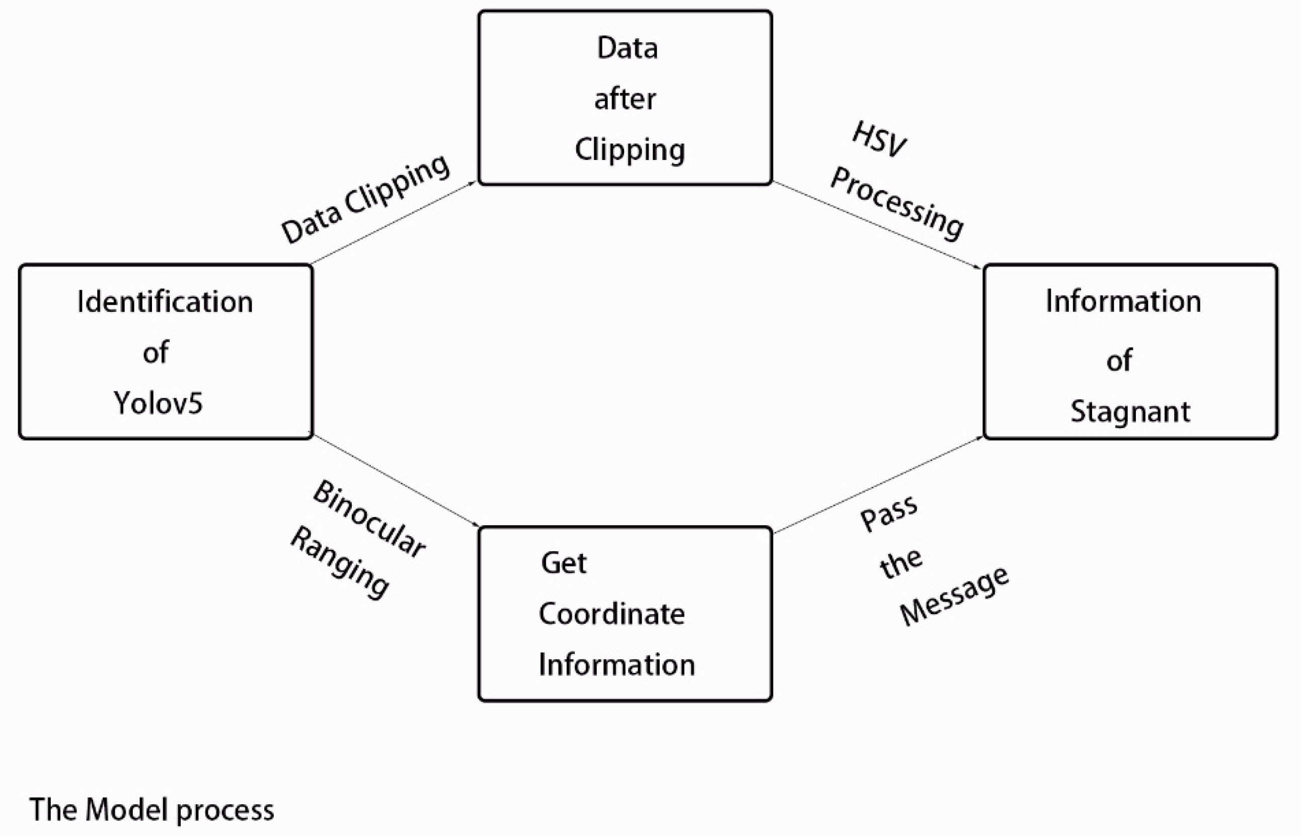
Part I: Using the improved YOLOV5 to identify the hydrops.
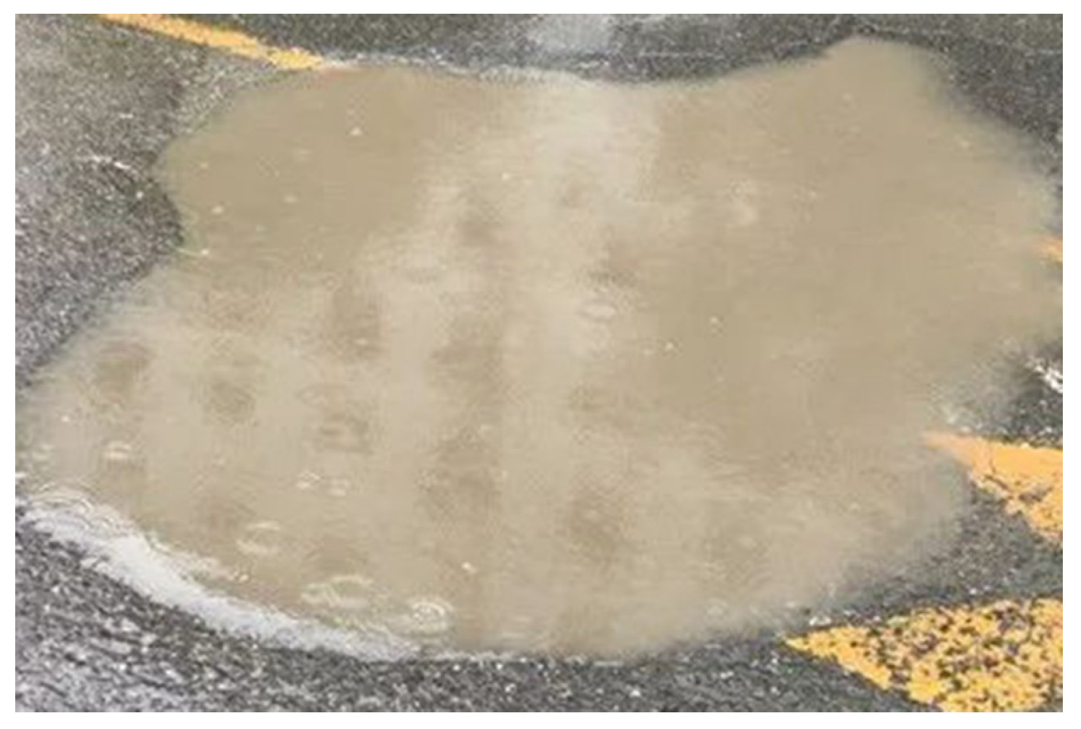
Part II: picture clipping, the above identified water frame for clipping. The binocular distance measurement material can obtain the actual distance in the actual situation and the three-dimensional coordinates of the key points needed at that time to obtain the real-time elevation data.
Part III: the outline obtained by the binarization of HSV and the image, the obfuscation processing and calculation by Opencv, and the contour area and circumference of the proportionally constrained contour obtained by binocular ranging are used to determine the current scene's inundation. The flow chart is shown in
Figure 1.
2. Materials and Methods
2.1. Images Data and Experimental Tool
This paper looks for 100 pictures of yellow water and shoots a video of yellow water. The video uses python scripts to capture images at a rate of five frames per second. The algorithms used for detection and classification (recognition) need to be trained, so images should be prepared for training. This work uses two schemes to use or generate training images. First, a still picture from the waterlogged category is used, and second, an extracted picture taken from one of the video recordings from the data set is generated and used. Then, each prepared image was enhanced in the first and second modes to enrich the data for better training process, and then all the material was flipped 90° 4 times using the action and batch processing method of PS software. The material enhancement technique used in this work [
30,
31] was used to obtain the last 500 pictures for training.
Use marking procedures during training steps. In this work, the conventional type of labeling is used [
32]. Traditional marking techniques are the most commonly used and can meet the training material requirements in most cases.
2.2. Improved Yolov5
2.2.1. Original Yolov5 Structure
YOLO (You only look once) [
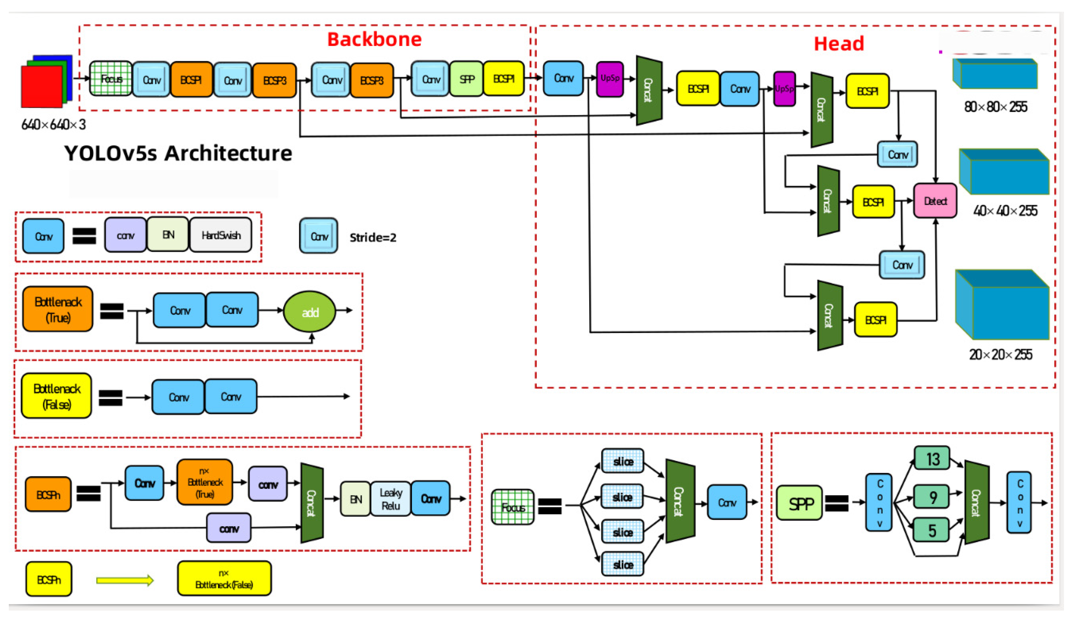
33] is used as a recognition algorithm. This algorithm is very popular and is called real-time object detector. Because of its speed and accuracy, the Yolov5 network structure mainly consists of the following parts: Backbone: New CSP-Darknet53, Neck: SPPF, New CSP-PAN, Head: YOLOv3 Head, Yolov5 Structure diagram is shown in
Figure 2.
The overall architecture of YOLOv5 is the same for different network sizes (n, s, m, l, x), but with different depths and widths for each submodule, dealing with depth_multiple and width_multiple parameters in the yaml file, respectively. Residual network can avoid the problem of disappearing gradient in deep network learning [
34]. In addition to the n, s, m, l and x versions, there are also n6, s6, m6, l6 and x6. The difference lies in that the latter is for pictures with a larger resolution, such as 1280x1280. Of course, there are some differences in structure. The former will only downsample to 32 times and use 3 prediction feature layers.
2.2.2. GAMAttention
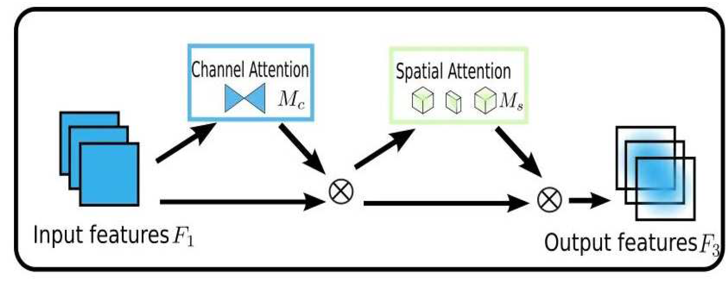
The target design of GAM is to reduce information reduction and amplify the mechanism of global unique interaction features, and optimize the channel attention module and spatial attention module in CBAM [
35]. The flow chart of GAM is shown as
Figure 3.
The main role of the channel attention module is to retain 3D information using 3D permutation, in which the relationship between the cross-dimensional channel and the space bar is amplified using a two-layer multi-layer perceptron.
In the spatial attention submodule, two convolution layers are used to reduce the spatial focus information, which solves the problem of overfitting and underfitting.
2.2.3. BoTNet Transformer
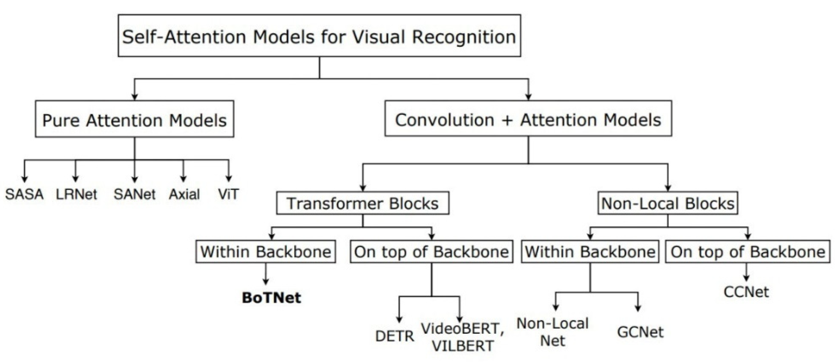
BoTNet brings self-attention to ResNet, very simple, but very powerful. Because it is not easy to obtain global information, CNN-based model pays more attention to the aggregation of local information. Transformer-based models are inherently capable of accessing global information. A simple way to use self-attention in computer vision is to directly replace the convolutional layer with multi-head self-attention (MHSA) [
36]. Currently, the users of self-attention in computer vision can be classified as
Figure 4:
2.3. Validation Matrix
Validation matrix Confusion matrix is used to evaluate the output of the model. The matrix consists of four blocks; TP, TN, FP and FN. TP(True Positive) : indicates that the positive class is predicted to be positive. If the true value is 0, the prediction is also 0. FN(False Negative) : predicts the positive class number as negative, the true value is 0, and the predicted value is 1; FP(False Positive) : The negative class was predicted as positive, the true value was 1, and the prediction was 0. TN(True Negative) : indicates that the negative class is predicted as the number of negative classes. If the true value is 1, the prediction is also 1. TP (true positive) is defined as when the model can correctly detect stagnant water, TN (true negative) is defined as when the model cannot correctly detect non-existent water, which was not measured in this work, FP (false positive) is defined as when the model incorrectly detects stagnant water, and FN (false negative) is defined as when the model fails to detect stagnant water. From the confusion matrix, the accuracy can be defined to evaluate the output of the model. It can be obtained from a comparison between the basic facts and the total blocks, as described by the following equation:
TP = true positive, FP= false positive, FN = missed positive.
2.4. RGB&HSV
RGB model is usually used to interpret color coding in visual information processing. However, in order to represent the subtle changes in the environment that trigger the regulation of pupil light reflex and DA/LA process, we use the HSV model. Compared with the supervised learning algorithm, the sensitivity improvement of the proposed model does not require additional computational resources and the image can be processed quickly.
2.4.1. Basic Principles of HSV
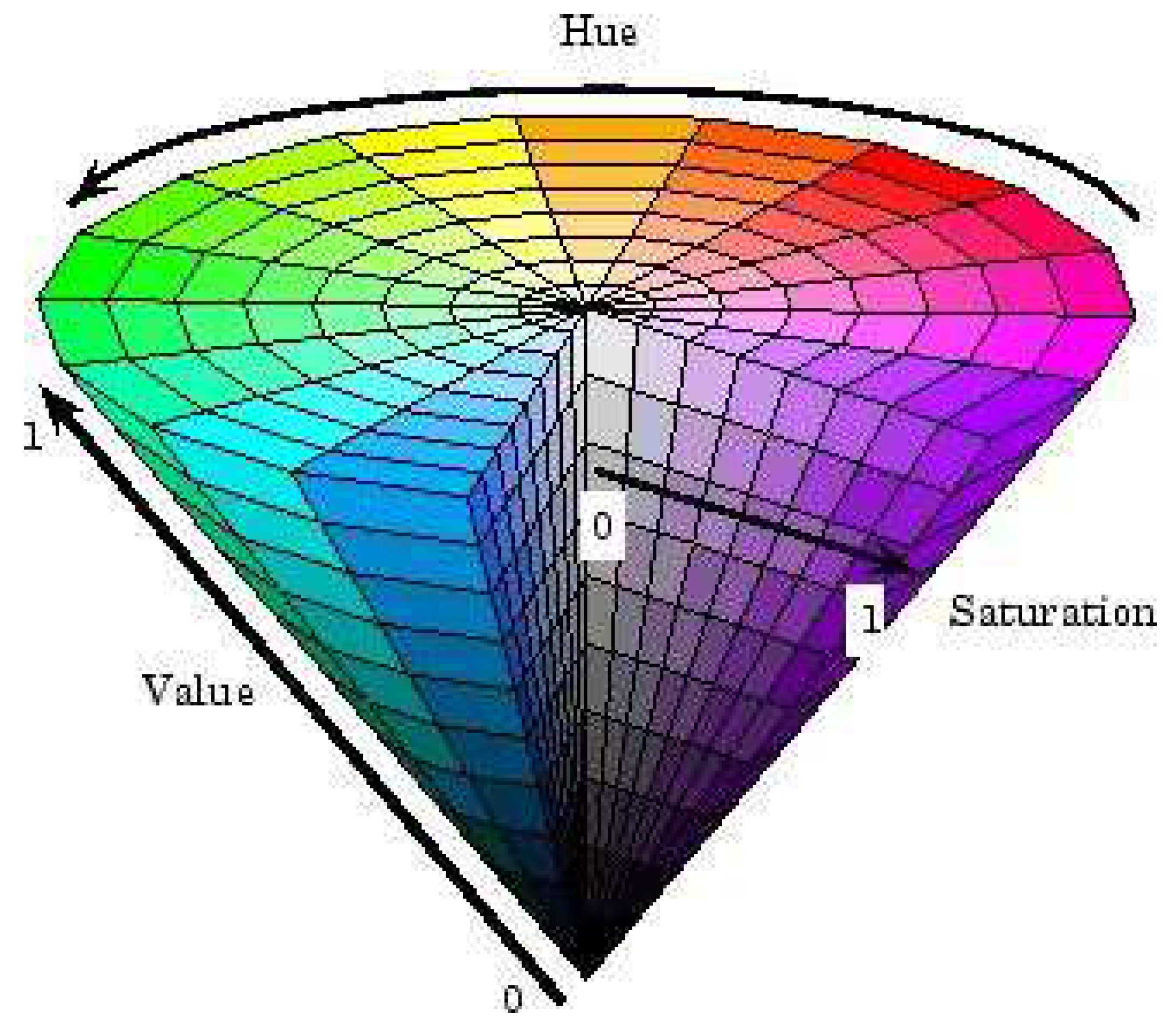
HSV(Hue, Saturation, Value) is Hue saturation (HSV) Color space was created by Alvy Ray Smith in 1978. Originally, it was designed to improve the color selection interface in computer graphics software, also known as Hexcone Model (see Baidu). In the HSV model, color is composed of Hue, Saturation and Value. HSV schematic diagram is shown as
Figure 5:
The channels of the HSV color space Q represent Hue, Saturation and Value respectively, and can directly express the brightness, hues and vividness of colors. The HSV color space can be described by a conical space model.
At the apex of the cone V=0, H and S are undefined, representing black, and at the center of the top surface of the cone V=max, S=0, H is undefined, representing white. When S= 1.v =1, any color represented by H is called a solid color: when S=0, saturation is 0, the color is lightest, the lightest is described as gray, the brightness of gray is determined by V, then H is meaningless, when V=0, the color is darkest, the darkest is described as black, then H and S are meaningless, no matter what the value is black.
The conversion process between them is as follows:
First, the number of components R, G and B is scaled to the range 0 to 1, that is, divided by 255, and then converted according to the following formula:
According to formula (3), (4) and (5), H, S and V are all between 0 and 1 after conversion, and H is between 0° and 360° (the calculation result may be less than 0, if it is less than 0, 360 will be added).
Suppose you want to convert pixels (11,43,46) respectively to RGB and convert them into the HSV model space:
2.5. Binocular Ranging
A series of systematic errors and error scenario errors will be generated by ToF method due to the principle and influence of measurement limiting external environmental factors [
37]. These errors will result in the error of image information obtained by the ToF depth camera for distortion[
38]. Binocu localization is more bionic in principle, has a wider range of applications and lower equipment cost [
39].The general steps of binocular distance measurement are:
Binocular calibration -> stereo correction (including distortion elimination) -> stereo matching -> parallax calculation -> depth calculation (3D coordinate) calculation.
The calibration of binocular camera not only needs to obtain the internal parameters of each camera, but also needs to measure the relative position between two cameras through calibration (that is, the translation vector t and rotation matrix R of the right camera relative to the left camera).
The calibration results are read into OpenCV for subsequent image calibration and matching.
Radial distortion and tangential distortion are generally modeled using polynomial functions, as shown below.
Radial distortion can be modeled as:
Tangential distortion can be modeled as:
where, x and y are normalized plane coordinates. According to the above modeling method, there are altogether 5 distortion parameters required:
In general, these 5 distortion factors are sufficient. For some cameras, higher order parameters may be required to model image distortion more accurately. For example:
From (6)-(11), the part of model can get accurate actual xyz and distance data.
2.6. Opencv Contour
2.6.1. Principles of Opencv Contour Acquisition
The basic principle of contour extraction: for a binary image with black background and white target, if a white point is found in the image, and its 8 neighborhood (or 4 neighborhood) is also white, it means that the point is the internal point of the target. If it is set as black, it will look like the interior is hollowed out. Otherwise, keep the white color unchanged. This point is the contour point of the target. Generally, before finding the contour, the image should be thresholding or Canny edge detection, and converted into a binary image. A curve of consecutive points having the same color (in a color picture) or intensity (a grayscale image is to be transformed into a binary image).
2.6.2. Contour Approximation Method
The contour approximation uses the Ramer-Douglas-Peucker(RDP) algorithm, which first simplifies the polyline by reducing the vertices of the polyline by a given scent value. Given the starting point and end point of the curve, the algorithm will first find the vertex with the greatest distance from the line connecting the two reference points. Let's call it the maximum point. If the maximum point is located at a distance less than the smell value, we automatically ignore all vertices between the starting point and the ending point, making the curve a straight line.
3. Results
3.1. Using Static Pictures for Training Data
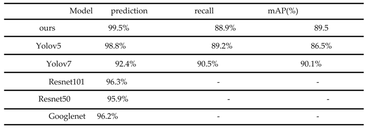
At this stage, extracted pictures were used as training image data,.After the train of Yolov5、Yolov7、Resnet and Goolenet,These experiments get a group of data compared with the improved Yolov5 model.All data of training as
Table 1.
The prediction rate of the improved Yolov5 is 7.1% higher than that of Yolov7 and 1.7% higher than that of Yolov5. The mAP is 3% higher than that of the traditional Yolov5, and the recall is slightly lower than that of other models. Although the recall and mAP of Yolov7 are slightly higher than that of the new model, the prediction rate of the improved YOLOV7 is significantly lower than that of other models. The improved Yolov5 has obvious improvements and advantages compared with other models.
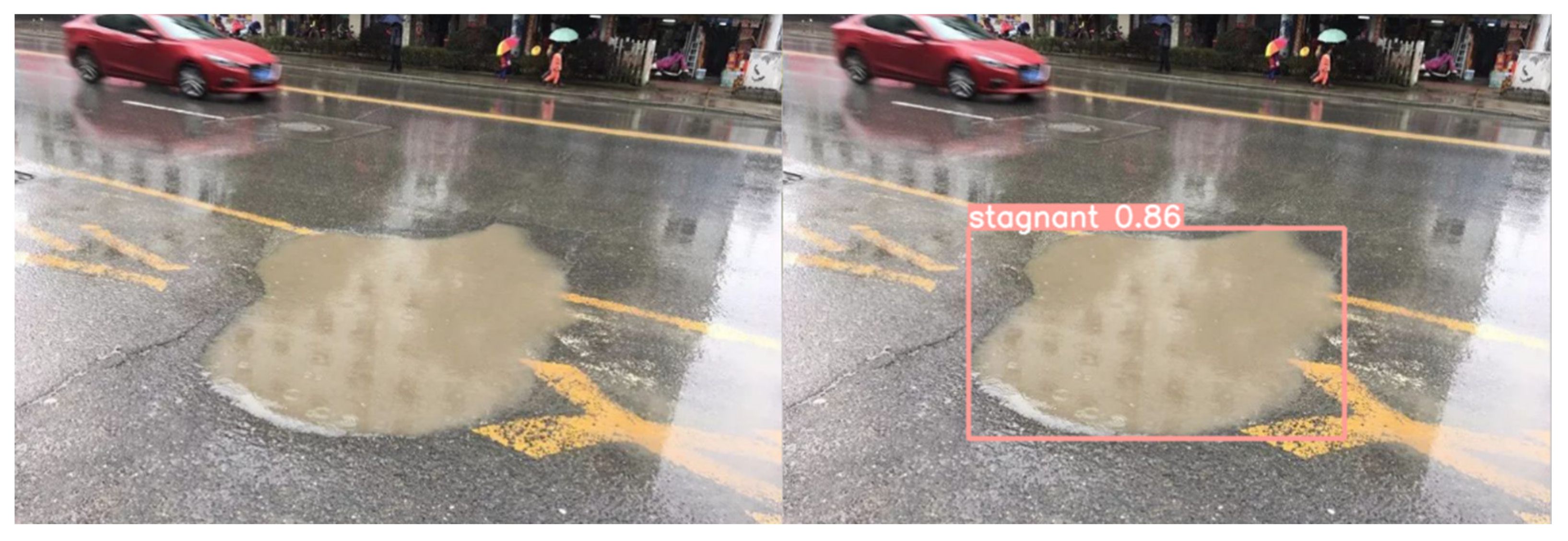
The weight trained by our method can be used to effectively identify water. The identification results are shown in
Figure 6.
3.2.cutting Materials
Although the identified picture can identify the water, if the subsequent processing continues, there will be many factors interference of backgrounds, reduce the later use efficiency, so we cut the required part of the box, reduce the influence factors as far as possible, and obtain a better effect for our contour area.
Figure 7.
The Material Cutting.
Figure 7.
The Material Cutting.
3.3. Comparison Whether with HSV
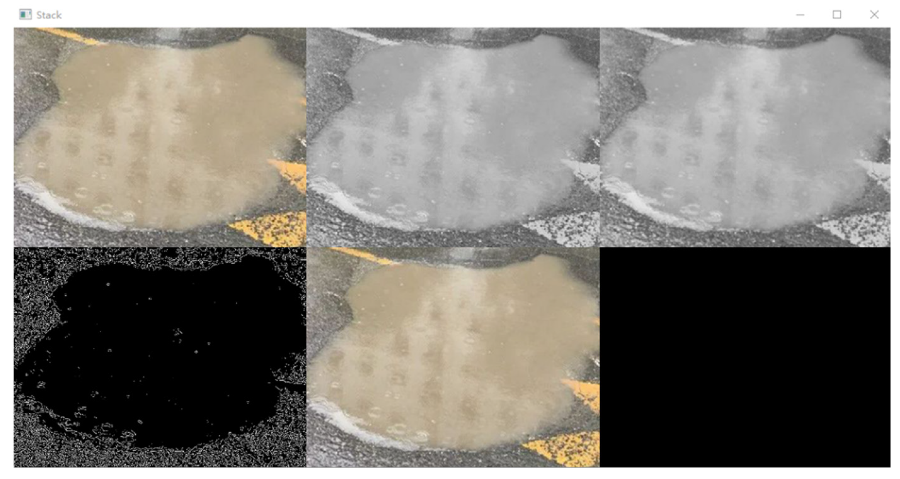
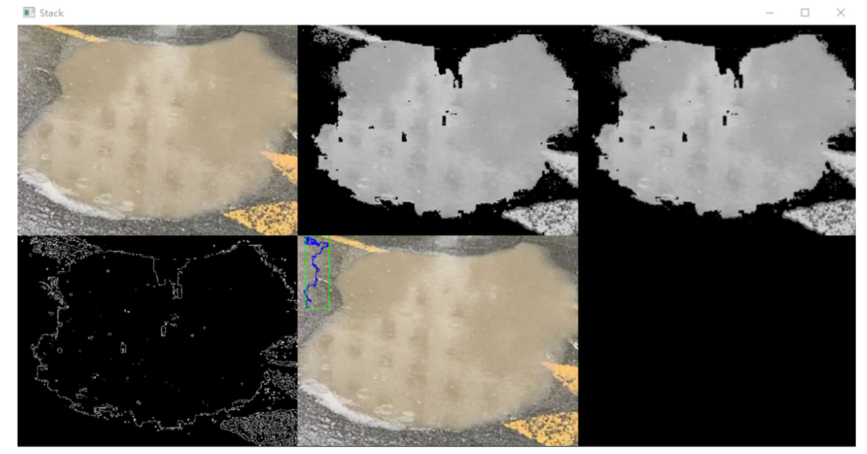
Before HSV processing and recognition, it is very necessary to carry out binarization and Gaussian blur processing in the contour recognition of computer. Without these treatments, the contours of the images are so poor that they cannot be prepared for recognition and analysis, and then we can use HSV processing method to screen and extract the color of the image. The threshold of yellow color used in the experiment was selected (LowerYellow = np.array([11, 43, 46]). UpperYellow = np.array([25, 255, 255])), which is then processed by the computer to clearly obtain the desired outline
Figure 8.
Material without HSV Process.
Figure 8.
Material without HSV Process.
It can be clearly seen from
Figure 9 and
Figure 10 that after color processing, there are obvious differences and contrasts between the second and third images of the two Figures. The HSV processed binarization, noise reduction and Gaussian blur have better contour display with fewer influencing factors. Compared with the first drawing in the second row, the final contour obtained will have much less invalid area and more delicate outline.
3.4. Get Data of Stagnant
This part is a step to calculate the result quantitatively. After calculating the area with the contour, Opencv calculates the actual proportion of the binocular distance measurement, and finally obtains a result of the actual area.
In this part, we still compare the results from the starting point of whether HSV processing is carried out or not. The results are shown in
Figure 11 and Figure 12:
The results of
Figure 10 and
Figure 11 show that there is a gap of accuracy. This is caused by the difference in the previous processing steps. We can see that
Figure 11 obtained after HSV processing are more delicate and have fewer influencing factors. Quantitatively, the area treated by HSV is
more correct and closer to the reality. Finally, the ratio of binocular ranging can be determined, and the real size of the processed data can be obtained.
4. Limitations and Future Developments
The analysis of limitations and future development is necessary. This experiment for the selection of data and the use of image processing technology for future development, such as strengthening the form of water in a particular area, water shape, water is universal everywhere that will be a huge and arduous project; As for the weight selection of Yolov7, there is a better possibility that the weight of 7 has not been discovered in this experiment due to the limited equipment. We can also combine the method with other classification algorithms or unsupervised learning. An adjustment or inference method may be proposed to optimize the accuracy of the method in this work. In addition, statistical hypothesis analysis can be carried out, using a variety of different recognition types such as cv tool recognition, tensorflow tool recognition.
In terms of technical extension, this technology can only be used as a simple water body analysis technology at present. In the future, it can be combined with GIS system to analyze the water body of a certain area. In this case, the server and video card support are more stringent than now.
5. Conclusions
This paper puts forward an idea and method of urban road inundation analysis. This paper takes the water that can be seen everywhere on the road as an example to analyze. In this method, improved YOLOv5 and conventional drawing methods were used to extract images as training data, and the accuracy of model recognition was 99.5%. After a series of techniques to get water body identification, cutting, actual distance, binary Gaussian blur and HSV image processing, finally get its image area circumference. In this way, it can get a general picture of the current water body. Therefore, we draw the following conclusions to summarize the role of the model:
1. Models with more accurate accuracy than traditional identification models
In the recognition part of this model, DAMAttention is used to improve the recognition focus and BoTNet to improve the constraint ability, so as to achieve more accurate recognition than traditional Yolov5 and other models.
2. Distributed real-time data acquisition model faster than traditional
In this model, the fixed-point data acquisition model carries out real-time data acquisition for a certain area, monitors the signs of important areas, and makes corresponding actions at the corresponding time.
3. More accurate models than traditional data
This model identifies and quantitatively detects water bodies, and uses binocular ranging to restrict the quantity, so as to achieve the maximum possible consistency with the actual data, so as to cooperate with the follow-up traditional GIS inundation analysis.
Author Contributions
All authors have equally contributed. All authors have read and agreed to the published version of the manuscript.
Funding
This study is funded by National Key R&D Program of China(No. 2021YFC3000200), the Research Programme of the Kunming Engineering Corporation Limited (No. DJ-HXGG-2021-04), the Key Research and Development Programme of Yunnan (No. 202203AA080010) as part of the Science and Technology Plan Project of Yunnan Provincial Department of Science and Technology, the Science and Technology Project of China Huaneng Group Research on Integrated Meteorology and Hydrology Forecasting System in Lancang River Basin (No:HNKJ21-HF241).
Conflicts of Interest
The authors declare no conflict of interest.
References
- Krestenitis, Y.N.; Androulidakis, Y.S.; Kontos, Y.N.; Georgakopoulos, G. Coastal inundation in the north-eastern mediterra-nean coastal zone due to storm surge events. J. Coast. Conserv. 2011, 15, 353–368. [Google Scholar] [CrossRef]
- Li Felipe Quintero Duque , Trevor Grout , Bradford Bates , Ibrahim Demir, Comparative analysis of performance and mechanisms of flood inundation map generation using Height Above Nearest Drainage.
- Oudin, L., Salavati, B., Furusho-Percot, C., Ribstein, P., Saadi, M. Hydrological impacts of urbanization at the catchment scale. J. Hydrol. 2018, 559, 774–786. [CrossRef]
- Hosseinzadehtalaei, P., Tabari, H., Willems, P. Climate change impact on shortduration extreme precipitation and intensity–duration–frequency curves over Europe. J. Hydrol. 2020, 590.
- Perini, L.; Calabrese, L.; Salerno, G.; Ciavola, P.; Armaroli, C. Evaluation of coastal vulnerability to flooding: Comparison of two different methodologies adopted by the Emilia-Romagna region (Italy). Nat. Hazards Earth Syst. Sci. 2016, 16, 181–194. [Google Scholar] [CrossRef]
- Mingfu Guan a, Kaihua Guo a, Haochen Yan a, Nigel Wright b,Bottom-up multilevel flood hazard mapping by integrated inundation modelling in data scarce cities.
- Li-Chiu Chang a, Jia-Yi Liou b, Fi-John Chang, Spatial-temporal flood inundation nowcasts by fusing machine learning methods and principal component analysis.
- Nkwunonwo, U., Whitworth, M., Baily, B. A review of the current status of flood modelling for urban flood risk management in the developing countries. Sci. Afr. 2020, 7, 1–16.
- Pengel, B.E. et al. Flood Early Warning System: Sensors and Internet. IAHS Red Book N 357, Floods: From Risk to Opportunity. pp.445-453, January 2013. ISBN 978-1-907161-35-3, IAHS Press. 20 January.
- Pyayt, A.L. et al. Machine Learning Methods for Environmental Monitoring and Flood Protection. World Academy of Science, Engineering and Technology, Issue 54, pp. 118–123, June 2011. http://waset.org/journals/waset/v54/v54-23.pdf .IjkDijk project.http://www.ijkdijk.eu. 20 June.
- Pyayt, A.L. et al. Artificial Intelligence and Finite Element Modelling for Monitoring Flood Defence Structures. Proc. 2011 IEEE.Workshop on Environmental, Energy, and Structural Monitoring Systems. Milan, Italy, September 2011, p. 1-7.
- Melnikova, N.B.; Shirshov, G.S.; Krzhizhanovskaya, V.V. Virtual Dike: multiscale simulation of dike stability. Procedia Computer Science, V. 4, p. 791-800, 2011.
- Melnikova, N.B. et al. Virtual Dike and Flood Simulator: Parallel distributed computing for flood early warning systems. Proc. International Conference on Parallel Computational Technologies (PAVT-2011). Publ. Centre of the South Ural State University. Chelyabinsk, p. 365-373. e/PaVT2011/short/139.pdf.
- Gouldby, B.; Krzhizhanovskaya, V.V.; Simm, J. Multiscale modelling in real-time flood forecasting systems: From sand grain to dike failure and inundation. Procedia Computer Science, V.1, p. 809, 2010. [CrossRef]
- Mordvintsev, A.; Krzhizhanovskaya, V.V.; Lees, M.; Sloot, P.M.A. Simulation of City Evacuation Coupled to Flood Dynamics. Proc. of the 6th International Conference on Pedestrian and Evacuation Dynamics, PED2012. Springer, 2013.
- Li, Ibrahim Demir, A comprehensive web-based system for flood inundation map generation and comparative analysis based on height above nearest drainage.
- Li, N. Qin, C.; Du, P. Optimization of China sponge city design: The case of Lincang Technology Innovation Park. Water 2018, 10, 1189. [CrossRef]
- Zhang, J.; Nong, C.; Yang, Z. Review of object detection algorithms based on convolutional neural network. J. Ordnance Equip.Eng. 2022, 43, 37–47. [Google Scholar]
- Girshick, R.; Donahue, J.; Darrell, T.; Malik, J. Rich Feature Hierarchies for Accurate Object Detection and Semantic Segmentation. In Proceedings of the 2014 IEEE Conference on Computer Vision and Pattern Recognition, Columbus, OH, USA, 23–28 June 2014; pp. 580–587. [Google Scholar]
- Girshick, R. Fast R-CNN. In Proceedings of the 2015 IEEE International Conference on Computer Vision (ICCV), Santiago, Chile, 7–13 December 2015; pp. 1440–1448. [Google Scholar]
- Ren, S.; He, K.; Girshick, R.; Sun, J. Faster R-CNN: Towards Real-Time Object Detection with Region Proposal Networks. IEEE,Trans. Pattern Anal. Mach. Intell. 2017, 39, 1137–1149. [Google Scholar] [CrossRef] [PubMed]
- Liu, W.; Anguelov, D.; Erhan, D.; Szegedy, C.; Reed, S.; Fu, C.Y.; Berg, A.C. SSD: Single Shot MultiBox Detector. Proceedings ofthe European Conferenceon Computer Vision; Springer International Publishing: Berlin/Heidelberg, Germany; 2016. [Google Scholar]
- Redmon, J.; Divvala, S.; Girshick, R.; Farhadi, A. You Only Look Once: Unified, Real-Time Object Detection. In Proceedings of the 2016 IEEE Conference on Computer Vision and Pattern Recognition (CVPR), Las Vegas, NV, USA, 27–30 June 2016; pp. 779–788. [Google Scholar]
- Redmon, J.; Farhadi, A. YOLO9000: Better, Faster, Stronger. In Proceedings of the 2017 IEEE Conference on Computer Vision and Pattern Recognition (CVPR), Honolulu, HI, USA, 21–26 July 2017; pp. 6517–6525. [Google Scholar]
- Redmon, J.; Farhadi, A. YOLOv3: An Incremental Improvement. arXiv arXiv:1804.02767, 2018.
- Bochkovskiy, A.; Wang, C.-Y.; Liao, H.-Y.M. YOLOv4: Optimal Speed and Accuracy of Object Detection. arXiv arXiv:2004.10934, 2020.
- Li, C.; Li, L.; Jiang, H.; Weng, K.; Geng, Y.; Li, L.; Ke, Z.; Li, Q.; Cheng, M.; Nie, W.; et al. YOLOv6:A Single-Stage Object Detection Framework for Industrial Applications. arXiv arXiv:2209.02976, 2022.
- Wang, C.-Y.; Bochkovskiy, A.; Liao, H.-Y.M. YOLOv7: Trainable bag-of-freebies sets new state-of-the-art for real-time object detectors. arXiv arXiv:2207.02696, 2022.
- Shf, P.; Zhao, C. Review on Deep based Object Detection. In Proceedings of the 2020 International Conference on Intelligent Computing and Human-Computer Interaction (ICHCI), Sanya, China, 4–6 December 2020; pp. 372–377. [Google Scholar]
- Liu, Z.; Jia, X.; Xu, X. Study of shrimp recognition methods using smart networks. Comput. Electron. Agric. 2019, 165, 104926. [Google Scholar] [CrossRef]
- Sonali Bhutad, Kailas Patil, Dataset of Stagnant Water and Wet Surface Label Images for Detection.
- Kuswantori, A.; Suesut, T.; Tangsrirat, W.; Nunak, N. Development of object detection and classification with YOLOv4 for similar and structural deformed fish. EUREKA Phys. Eng. 2022, 2, 154–165. [Google Scholar]
- Jiang Du, Zheng Z, Li G, Sun Y, Kong J, Jiang G, et al. Gesture recognition based on binocular vision. Cluster Comput 2019;22(S6):13261–71. [CrossRef]
- Redmon, J.; Divvala, S.; Girshick, R.; Farhadi, A. You only look once:Unified, real-time object detection, in: 2016 IEEE Conference on Computer Vision and Pattern Recognition, CVPR, 2016, pp. 779–78.
- Yichao Liu, Zongru Shao, Nico Hoffmann. Global Attention Mechanism: Retain Information to Enhance Channel-Spatial Interactions. arXiv:2112.05561v1 [cs.CV] 10 Dec 2021.
- Aravind Srinivas,Tsung-Yi Lin,Niki Parmar,Jonathon Shlens,Pieter Abbeel, Ashish Vaswani,UC Berkeley,Google Research. Bottleneck Transformers for Visual Recognition. {aravind}@cs.berkeley.edu.
- Lu C, Song Y, Wu Y, Yang M. 3D information acquisition and error analysis based on ToF Computational imaging. Infrared Laser Eng 2018;47:1–7. [CrossRef]
- Li Z, Yan S, Liu Y, Guo Y, Hong T, Lu¨ S. Error analysis and compensation method for ToF depth-sensing camera. Mod Electron Tech 2021;44:50–5.
- He, K.; Zhang, X.; Ren, S.; Sun, J. Deep residual learning for image recognition, in: 2016 IEEE Conference on.
- Computer Vision and Pattern Recognition, CVPR, 2016, pp. 770–778, http://dx.doi.org/10.48550/arXiv.1512.03385.
|
Disclaimer/Publisher’s Note: The statements, opinions and data contained in all publications are solely those of the individual author(s) and contributor(s) and not of MDPI and/or the editor(s). MDPI and/or the editor(s) disclaim responsibility for any injury to people or property resulting from any ideas, methods, instructions or products referred to in the content. |
© 2023 by the authors. Licensee MDPI, Basel, Switzerland. This article is an open access article distributed under the terms and conditions of the Creative Commons Attribution (CC BY) license (http://creativecommons.org/licenses/by/4.0/).
