Extended Laplace Power Series Method for Solving Non-linear Caputo Fractional Volterra Integro-differential Equations

In this paper, we compile the fractional power series method and the Laplace transform to design a new algorithm for solving the fractional Volterra integro-differential equation. For that, we assume the Laplace power series (LPS) solution in terms of power q=1m,m∈Z+, where the fractional derivative of order α=qγ for which γ∈Z+. This assumption will help us to write the integral, the kernel, and the nonhomogeneous terms as a LPS with the same power. The recurrence relations for finding the series coefficients can be constructed using this form. To demonstrate the algorithm's accuracy, the residual error is defined and calculated for several values of the fractional derivative. Two strongly nonlinear examples are discussed to provide the efficiency of the algorithm. The algorithm gains powerful results for this kind of problem. Under Caputo meaning the obtained results are illustrated numerically, and graphically. Geometrically, the behavior of the solution declares that the changing of the fractional derivative parameter values' in their domain alters the style of the attained solution in a symmetrical meaning and fully coinciding to the ordinary derivative value'. From these simulations, the results report that the recommended novel algorithm is a straightforward, accurate, and superb tool to generate analytic-approximate solutions for Integral, and integro-differental equations of fractional order.

Keywords:

Subject: Computer Science and Mathematics - Applied Mathematics

1. Introduction

Fractional calculus (FC) is a mathematical discipline that dates back 300 years, defined in the 19th century by Rieman and Liouville as “the generalization of the ordinary derivative to non-integer values”, and was later developed by Euler, Liouville, and Abel (1823). For more details, see [1,2,3]. In the last decades, FC starts to attract much more attention from researchers. It was found that different, particularly interdisciplinary applications can be superbly modeled with the help of fractional derivatives. For instance, robotics, nonlinear oscillation of earthquakes, control theory, signal processing, and viscoelasticity [4,5,6,7]. For more details and applications of FC, we refer the reader to [8,9,10,11,12,13,14]. Since the ordinary differential is a local operator, but the fractional order differential operator is non-local, the non-local property is considered the most significant aspect of using fractional differential equations (FDEs), which indicates the following state of a phenomenon does not rely only upon its current state but considers its historical states as well. For this reason, FDEs have drawn great attention from researchers for their realism in the interpretation of real-world phenomena and it has become a more popular mathematical discipline: such as circuit systems [15], electrochemistry of corrosion [16], heat conduction [17], optics and signal processing [18], probability and statistics [19], inviscid fluid [20], fluid flow [21], and so on. In the literature, eminent researchers have introduced and developed various ways to define the fractional derivatives (FD), such as Atangana–Baleanu, Riemann– Liouville, Abel, Weyl, Riesz, Caputo–Fabrizio, and Caputo operators. The Riemann–Liouville, and Caputo FDs are the most popular, they give a high degree of freedom in the description and simulation of the physical phenomena compared with ordinary derivatives. To learn about these FDs, (see [22,23,24,25,26,27,28]).

Various mathematical forming of science and engineering phenomena involve linear and non-linear differential equations, Integral equations, or Integro-differential equations (DEs, IEs, IDEs) that play a vital role to simulate a wide range of both linear and non-linear phenomena in varied science and engineering fields. However, when converting these phenomena to one of DEs, IEs, or IDEs some of them are complicated and cannot be treated with the help of ordinary calculus. In this regard, many scientists have concentrated on employing FDEs and fractional IDEs (FIDEs) as convenient tools in modeling the phenomenon and play an important role in exploring solutions utilizing varied methods, which is in line with the rapid growth in explaining the various phenomena originating from the natural sciences more accurately than ordinary DEs. But, there remain challenges to solving the non-linear models of such phenomena theoretically or numerically. Recently, many researchers have devoted more effective methods to provide a solution, approximate, analytical, numerical, or exact to such models. Exploring the analytic solution of FDEs and FIDEs is difficult hard in most cases. Even though, abundant efforts had been introduced recently to develop emerging numerical and approximate-analytical techniques for finding out the solutions to linear and nonlinear fractional problems. Among these methods, reproducing kernel Hilbert space method [29], the Haar wavelet method [30], the Adomian decomposition method [31], the homotopy analysis method [32], the finite difference method [33], the Taylor series expansion method [34], collocation method [35], the power series method [36,37,38], and the Aboodh transform decomposition method [39]. One of the novel and efficient techniques for generating analytic-approximate of wide classes of FDEs and FIDEs is the Laplace fractional power series (LFPS) method. LFPS approach had been suggested as a modern algorithm which is a mixture of two strong approaches, fractional power series (FPS) and Laplace transform (LT). The LFPS algorithm is a considerable algorithm to be appropriate for handling several linear and non-linear fractional models and investigating their solutions: such as time-fractional Swift-Hohenberg equations [40], time-fractional Black–Scholes option pricing equations [41], time-fractional Kolmogorov and Rosenau–Hyman models [42], temporal time-fractional gas dynamics equations [43], time-fractional generalized biology population model [44], and fractional reaction–diffusion for bacteria growth model [45].

Motivated by the aforementioned works, this article extends the application of LPSM for solving non-linear FIDEs in the Volterra sense, as shown in the underlying form.

D_{t}^{α} u (t) = f (t) + \int_{0}^{t} k (x, t) g (u (x)) d x, α \in (0,1], t \geq 0,

(1)

where

α

, is the parameter defining the Caputo-FD, the functions

f (t)

k (x, t)

are continuous real-valued functions, and

g (u (x))

, is the non-linear function of

u (x) .

In the Volterra sense, the solution of FIDEs is crucial for describing the pattern of linear and non-linear physical phenomena, particularly, the phenomena excited in harmony or to evaluate the probabilistic response of randomly-excited analytical models, the dynamics of nuclear reactors, and so forth. A functional expansion of a dynamic, nonlinear, and time-invariant functional is referred to as Volterra Series.

The main contribution of this work is to design a modern modified algorithm to generate the analytic-approximate solutions of the non-linear fractional Volterra integro–differential equation (FVIDE) in the framework of employing Caputo-FD. This kind of FD is chosen in the present analysis due to its simplicity in handling both linear and non-linear FIDEs and its compatibility with initial conditions, that is; when solving FDEs or FIDEs, initial conditions are often involved. As well, the Caputo-FD handles initial conditions naturally and allows for a direct and consistent incorporation of these conditions into the formulation of the problem. Furthermore, it satisfies the causality property, which means that the value of FD at a particular time depends only on the values of the function up to that time. This property aligns well with the physical interpretation of FDs in many applications, where the current behavior of a system depends on its history. The principle of exploring approximate solutions is discussed. The remaining sections of this work are structured as follows: In section two, some elementary results of FC theory and LT features are presented. Next, a modified LFPS algorithm to examine and establish the approximate solution of the target model (1) is presented in section three. In section four, the simplicity, potential, and accuracy of the recommended scheme are provided by two non-linear FVIDEs with appropriate initial conditions. Toward the end, some concluding remarks are drawn in the last section.

2. Preliminaries and Basic Concepts

FC theory deals with generalizing the concepts of differentiation and integration to non-integer orders. It introduces the notion of FDs and FIs, allowing for the analysis and modeling of phenomena that exhibit fractal behavior, memory effects, and long-range dependencies. The Caputo-FD is one of the widely used definitions in FC theory. In this section, we retrieved the basic definitions and features of FC theory, as well as the LT operator and FPS method within the framework of the Caputo-FD.

Definition 1.

[2] The

α

th-FD in the Caputo sense of

u \in C_{μ}, μ \geq - 1,

denoted by

D_{t}^{α}

, and given by

D_{t}^{α} u (t) = \{\begin{array}{l} u^{(n)} (t), & α = 0 \\ J_{t}^{n - α} (u^{(n)} (t)), & α \in (n - 1, n), n \in N \end{array} .

(2)

Theorem 1.

[47] Assume that the transform function

U (ξ) = L \{u (t)\}

, could be given in the following fractional series expansion(FSE):

U (ξ) = \sum_{n = 0}^{\infty} \frac{u_{n}}{ξ^{n α + 1}}, ξ > 0, α \in (0, 1],

(3)

where the coefficients

u_{n} = (D_{t}^{n α} u (t)) (0) .

Definition 2.

[47] Suppose that

u (t)

is of exponential order

γ

, and piecewise continuous on

[0, \infty)

, then the LT of

u (t)

is defined as:

U (ξ) = L \{u (t)\} = \int_{0}^{\infty} u (t) e^{- ξ t} d t, ξ > γ,

(4)

and the inverse LT of the transform function

U (ξ)

is defined as:

L^{- 1} \{U (ξ)\} = u (t) = \int_{δ - i \infty}^{δ + i \infty} U (ξ) e^{ξ t} d ξ, δ = R e (ξ) > δ_{0} .

(5)

Lemma 1.

Let

u_{1} (t)

, and

u_{2} (t),

are two piecewise continuous on

[0, \infty)

and be of exponential order. Then, the following are hold for the constants

c_{1}

c_{2}

, and

U_{1} (ξ) = L \{u_{1} (t)\}, U_{2} (ξ) = L \{u_{2} (t)\}

$L \{c_{1} u_{1} (t) + c_{2} u_{2} (t)\} = c_{1} U_{1} (ξ) + c_{2} U_{2} (ξ)$ .
$L^{- 1} \{c_{1} U_{1} (ξ) + c_{2} U_{2} (ξ)\} = c_{1} u_{1} (t) + c_{2} u_{2} (t) .$
$\lim_{ξ \to \infty} ξ U (ξ) = u (0)$ .
$L \{D_{t}^{α} u (t)\} = ξ^{α} U (ξ) - \sum_{k = 0}^{n - 1} ξ^{α - k - 1} u^{(k)} (0), α \in (n - 1, n], n \in N .$

Theorem 2.

[47] Assume that the transform function

U (ξ) = L \{u (t)\}

, could be expanded in a FSE (5). If

|ξ L [D_{t}^{(n + 1) α} u (t)]| \leq l

, on

(0, s]

where

0 < α \leq 1

. Then, the remainder of the new series form in Theorem 2, satisfies the following inequality:

|R_{n} (ξ)| \leq \frac{l}{ξ^{1 + (n + 1) α}}, 0 < ξ \leq s .

(6)

3. Principle of the LFPS Algorithm

The LFPS scheme is analytic-numeric algorithm specifically extended to deal with arising FDEs, and FPDEs in diverse linear and non-linear dynamical phenomena. This algorithm depends on the investigation of the series solution of the target problem in a new space called Laplace space with the simulation of the generalized arbitrary order Taylor series to find out the unknown components of the suggested series solution. The proposed scheme has sensational merits and superb capability to handle non-linear terms profitably without no inserting any physical hypotheses of the studied models. In this segment, a modified algorithm of LFPS scheme is developed for determining accurate analytic-approximate solutions of the certain class of FIDEs. In this context, let us consider the non-linear FVIDE (1) subject to the initial condition

u (0) = β .

It is needful to start with the following theorem that is required in the strategy of solving the target equation (1).

Theorem 3.

Suppose that for

ξ > 0, V (ξ) = \sum_{i = 0}^{n} \frac{v_{i}}{ξ^{i q + 1}}

, and

W (ξ) = \sum_{i = 0}^{m} \frac{ω_{i}}{ξ^{i q + 1}}

, then

V (ξ) W (ξ) = \sum_{i = 0}^{m + n} ξ^{- q i - 2} \sum_{j = \min [0, n]}^{\max [j, m]} v_{j} ω_{i - j}

Proof.

Define

δ (0) = 1, δ (i) = 0

for

i = 1,2, 3, \dots .

The product of the two series gives

\sum_{i = 0}^{n} \frac{v_{i}}{ξ^{i q + 1}} \sum_{i = 0}^{m} \frac{ω_{i}}{ξ^{i q + 1}} = \sum_{i = 0}^{n} \sum_{j = 0}^{m} v_{i} ω_{j} ξ^{- q (i + j) - 2} = \sum_{k = 0}^{n + m} \sum_{i = 0}^{n} \sum_{j = 0}^{m} v_{i} ω_{j} ξ^{- q (i + j) - 2} δ (k - (i + j)) = \sum_{k = 0}^{n + m} \sum_{i = 0}^{n} v_{i} [\sum_{j = 0}^{m} ω_{j} ξ^{- q (i + j) - 2} δ (j - (k - i))],

Since

δ (j - (k - i)) = 1

only if

j - (k - i) = 0

, which happened at

j = k - i

. Then

\sum_{j = 0}^{m} ω_{j} ξ^{- q (i + j) - 2} δ (j - (k - i)) = ω_{k - i} ξ^{- q k - 2} .

But

0 \leq k - i \leq m \Rightarrow k - m \leq i \leq k

, and

0 \leq i \leq n

. So that

\max [0, k - n] \leq i \leq \min [k, m]

□

Now, to solve FVIDE (1), we should transform it into the Laplace space as follows:

U (ξ) = \frac{u (0)}{ξ} + F (ξ) + \frac{1}{ξ^{α}} (L \{k (t)\} . L \{g (u (t))\}) .

(7)

Herein, let the order of Caputo-FD

α = γ q

, where

q = \frac{1}{m}, m \in Z^{+}, γ \in Z^{+}

such that if

α = 0.9 = γ \times q = 9 \times \frac{1}{10}

The proposed solution of (7) has the FSE form:

U (ξ) = \sum_{i = 0}^{\infty} \frac{u_{i}}{ξ^{i α + 1}},

(8)

provided that

u (0) = \lim_{ξ \to \infty} ξ U (ξ) = β

. Thus, the

J

-th truncated FSE form

U_{j} (ξ)

, could be expressed as:

U_{J} (ξ) = \frac{β}{ξ} + \sum_{i = 1}^{J} \frac{u_{i}}{ξ^{i α + 1}} .

(9)

Let

f (t)

and

k (t)

be analytic functions, then its LT can be written as

F (s) = \sum_{i = 0}^{J} \frac{f_{i}}{ξ^{q i + 1}}

and

L \{k (t)\} = \sum_{i = 0}^{J} \frac{k_{i}}{ξ^{q i + 1}}

. Then, by substitution these expansions series with FSE (9) into Equation (7), we get

\sum_{i = 1}^{J} \frac{u_{i}}{ξ^{q i + 1}} = \frac{1}{ξ^{γ q}} \sum_{i = 0}^{J} \frac{f_{i}}{ξ^{q i + 1}} + \frac{1}{ξ^{γ q}} \sum_{i = 0}^{J} \frac{k_{i}}{ξ^{q i + 1}} \sum_{i = 0}^{N} \frac{g_{i}}{ξ^{q i + 1}} .

(10)

Using Theorem 3, Equation (10) becomes as follows:

\sum_{i = 1}^{J} \frac{u_{i}}{ξ^{q i + 1}} = \frac{1}{ξ^{γ q}} \sum_{i = 0}^{J} \frac{f_{i}}{ξ^{q i + 1}} + \frac{1}{ξ^{γ q}} \sum_{i = 0}^{J + N} \frac{1}{ξ^{q i + 2}} \sum_{j = m a x [0, J]}^{m i n [i, N]} k_{i} g_{i - j} = \sum_{i = 0}^{J} \frac{f_{i}}{ξ^{q (i + γ) + 1}} + \sum_{i = 0}^{J + N} \frac{1}{ξ^{q (i + \frac{1}{q} + γ) + 1}} \sum_{j = m a x [0, J]}^{m i n [i, N]} k_{i} g_{i - j} .

(11)

Multiply Equation (11) by

ξ^{m q + 1}

for

m = 1,2, \dots J

, we have

\sum_{i = 1}^{J} \frac{u_{i}}{ξ^{q (i - m)}} = \sum_{i = 0}^{J} \frac{f_{i}}{ξ^{q (i + γ - m)}} + \sum_{i = 0}^{J + N} \frac{1}{ξ^{q (i + \frac{1}{q} + γ - m)}} \sum_{j = m a x [0, J]}^{m i n [i, N]} k_{i} g_{i - j} .

(12)

By taking the limit of the obtained Equation (12) as

ξ \to \infty

, such that

\lim_{ξ \to \infty} (\sum_{i = 1}^{J} \frac{u_{i}}{ξ^{q (i - m)}} - \sum_{i = 0}^{J} \frac{f_{i}}{ξ^{q (i + γ - m)}} - \sum_{i = 0}^{J + N} \frac{1}{ξ^{q (i + \frac{1}{q} + γ - m)}} \sum_{j = m a x [0, J]}^{m i n [i, N]} k_{i} g_{i - j}) = 0 .

(13)

Then, for the first, second, and third sums respectively; let

i = m, i = m - γ

, and

i = m - \frac{1}{q} - γ

. We have

u_{m} = f_{m - γ} + \sum_{j = \max [0, J]}^{\min [m - \frac{1}{q} - γ, N]} g_{j} k_{m - \frac{1}{q} - γ - j}, m = 1,2, 3, \dots

(14)

Thus, the proposed solution of (7) could be reformulated in the following FSE form:

U_{j} (ξ) = \frac{β}{ξ} + \sum_{i = 1}^{J} (f_{i - γ} + \sum_{j = \max [0, J]}^{\min [i - \frac{1}{q} - γ, N]} g_{j} k_{i - \frac{1}{q} - γ - j}) \frac{1}{ξ^{i α + 1}} .

(15)

Correspondingly, by performing the inverse LT operator on both sides of (15), one can reach the following analytic-approximate series solution of FVIDE (1) along with the given initial condition.

u (t) = L^{- 1} \{\frac{β}{ξ} + \sum_{i = 1}^{J} (f_{i - γ} + \sum_{j = \max [0, J]}^{\min [i - \frac{1}{q} - γ, N]} g_{j} k_{m - \frac{1}{q} - γ - j}) \frac{1}{ξ^{i α + 1}}\} = β + \sum_{i = 1}^{J} (f_{i - γ} + \sum_{j = \max [0, J]}^{\min [i - \frac{1}{q} - γ, N]} g_{j} k_{m - \frac{1}{q} - γ - j}) \frac{t^{q i}}{Γ (q i + 1)} .

(16)

4. Illustrated Examples

In this section, the LFPS algorithm is implemented to investigate analytical-approximate solutions of non-linear FVIDEs using Caputo-FD. Some graphical and numerical simulations are illustrated to show the performance and accuracy of our recommended algorithm. In this portion, we utilize Mathematica package 12 to perform computations.

Example 1.

Consider the following non-linear FVIDE:

D_{t}^{α} u (t) = \frac{3}{2} e^{t} - \frac{1}{2} e^{3 t} + \int_{0}^{t} e^{t - x} u^{3} (x) d x, 0 < α \leq 1,

(17)

subject to initial condition

u (0) = 1

. The exact solution of the system of non-linear FVIDE (17) at

α = 1

u (t) = e^{t}

, [46].

Following the process of the proposed algorithm in the last. Running LT into (17), we get

U (ξ) = \frac{u (0)}{ξ} + \frac{3}{2 ξ^{α}} L \{e^{t}\} + \frac{1}{2 ξ^{α}} L \{e^{3 t}\} + \frac{1}{ξ^{α}} L \{e^{t}\} \times L \{u^{3} (t)\} .

(18)

Utilizing the following series expansions:

L \{e^{t}\} = \sum_{i = 0}^{J} \frac{1}{ξ^{q i + 1}} = \sum_{i = 0}^{J} \frac{f_{i}}{ξ^{q i + 1}}, q i \in Z^{+}, L \{e^{3 t}\} = \sum_{i = 0}^{J} \frac{{(3)}^{q i}}{ξ^{q i + 1}} = \sum_{i = 0}^{J} \frac{c_{i}}{ξ^{q i + 1}}, q i \in Z^{+},

(19)

and

L \{u^{3} (t)\} = L \{{(L^{- 1} U (ξ))}^{3}\} = L \{{(\sum_{i = 0}^{J} \frac{u_{i}}{Γ (q i + 1)} t^{q i})}^{3}\} .

(20)

where

{(\sum_{i = 0}^{J} \frac{u_{i} t^{q i}}{Γ (q i + 1)})}^{3} = \sum_{i = 0}^{3 J} t^{q i} \sum_{j = \max [0, J]}^{\min [i, 2 J]} \frac{u_{i - j}}{Γ (q (i - j) + 1)} \sum_{v = \max [0, J]}^{\min [j, J]} \frac{u_{v} u_{j - v}}{Γ (v q + 1) Γ (q (j - v) + 1)} .

(21)

By performing LT operator into both sides of (21), we get

L \{{(\sum_{i = 0}^{J} \frac{u_{i}}{Γ (q i + 1)} t^{q i})}^{3}\} = \sum_{i = 0}^{3 J} \frac{Γ (q i + 1)}{ξ^{q i + 1}} \sum_{j = \max [0, J]}^{\min [i, 2 J]} \frac{u_{i - j}}{Γ (q (i - j) + 1)} \sum_{v = \max [0, J]}^{\min [j, J]} \frac{u_{v} u_{j - v}}{Γ (v q + 1) Γ (q (j - v) + 1)} .

(22)

Using Theorem 3, we have

L \{e^{t}\} \times L \{u^{3} (t)\} = \sum_{i = 0}^{J} \frac{f_{i}}{ξ^{q i + 1}} \sum_{i = 0}^{3 J} \frac{Γ (q i + 1)}{ξ^{q i + 1}} \sum_{j = \max [0, J]}^{\min [i, 2 J]} \frac{u_{i - j}}{Γ (q (i - j) + 1)} \sum_{v = \max [0, J]}^{\min [j, J]} \frac{u_{v} u_{j - v}}{Γ (v q + 1) Γ (q (j - v) + 1)} = \sum_{i = 0}^{4 J} \frac{1}{ξ^{q i + 2}} \sum_{n = \max [0, J]}^{\min [i, 3 J]} f_{i - n} Γ (n q + 1) \sum_{j = \max [0, J]}^{\min [i, 2 J]} \frac{u_{i - j}}{Γ (q (i - j) + 1)} \sum_{v = \max [0, J]}^{\min [j, J]} \frac{u_{v} u_{j - v}}{Γ (v q + 1) Γ (q (j - v) + 1)} .

(23)

By substitute

ξ^{α} = ξ^{γ q}

, the

j

-th truncated Laplace residual error function (L-REF) of the series form for the Laplace equation (18) can be given as:

L \{{R e s}_{U_{J}} (ξ)\} = \sum_{i = 1}^{J} \frac{u_{i}}{ξ^{q i + 1}} - \frac{3}{2} \sum_{i = 0}^{J} \frac{f_{i}}{ξ^{q (i + γ) + 1}} + \frac{1}{2} \sum_{i = 0}^{J} \frac{c_{i}}{ξ^{q (i + γ) + 1}} - \sum_{i = 0}^{4 J} \frac{1}{ξ^{q (i + γ + \frac{1}{q}) + 1}} \sum_{n = \max [0, J]}^{\min [i, 3 J]} f_{i - n} Γ (n q + 1) \sum_{j = \max [0, J]}^{\min [i, 2 J]} \frac{u_{i - j}}{Γ (q (i - j) + 1)} \sum_{v = \max [0, J]}^{\min [j, J]} \frac{u_{v} u_{j - v}}{Γ (v q + 1) Γ (q (j - v) + 1)} .

(24)

Multiply both sides of Equation (24) by the factor

ξ^{m α + 1}

, and take the limit as

ξ \to \infty

, we have

\underset{ξ \to \infty}{l i m} ξ^{m α + 1} L \{{R e s}_{U_{J}} (ξ)\} = \underset{ξ \to \infty}{l i m} \sum_{i = 1}^{J} \frac{u_{i}}{ξ^{q (i - m)}} - \frac{3}{2} \sum_{i = 0}^{J} \frac{f_{i}}{ξ^{q (i + γ - m)}} + \frac{1}{2} \sum_{i = 0}^{J} \frac{c_{i}}{ξ^{q (i + γ - m)}} - \sum_{i = 0}^{4 J} \frac{1}{ξ^{q (i + γ + \frac{1}{q} - m)}} \sum_{n = \max [0, J]}^{\min [i, 3 J]} f_{i - n} Γ (n q + 1) \sum_{j = \max [0, J]}^{\min [n, 2 J]} \frac{u_{n - j}}{Γ (q (n - j) + 1)} \sum_{v = \max [0, J]}^{\min [j, J]} \frac{u_{v} u_{j - v}}{Γ (v q + 1) Γ (q (j - v) + 1)} .

(25)

Then, by solving

\underset{ξ \to \infty}{l i m} ξ^{m α + 1} L \{{R e s}_{U_{J}} (ξ)\} = 0

, we get the following recurrence formula:

u_{m} = \frac{3}{2} f_{m - γ} - \frac{1}{2} c_{m - γ} + \sum_{n = \max [0, J]}^{\min [m - \frac{1}{q} - γ, 3 J]} f_{m - \frac{1}{q} - γ - n} Γ (n q + 1) \sum_{j = \max [0, J]}^{\min [n, 2 J]} \frac{u_{n - j}}{Γ (q (n - j) + 1)} \sum_{v = \max [0, J]}^{\min [j, J]} \frac{u_{v} u_{j - v}}{Γ (v q + 1) Γ (q (j - v) + 1)} .

(26)

For

m = γ, γ + 1, γ + 2, \dots M .

In case

α = 0.9

, we choose

q = \frac{1}{10}, γ = 9

, then

u_{0} = 1, u_{i} = 0;

for

i = 1,2, \dots, 8

. Then, the recurrence formula (26) gives the following first nonzero coefficients:

u_{9} = u_{19} = 1, u_{28} = 3, u_{29} = - 2, u_{37} = \frac{3 Γ (\frac{14}{5})}{Γ {(\frac{19}{10})}^{2}} .

Thus, the analytic-approximate series solution of FVIDE (17) becomes as:

u (t) = L^{- 1} [\sum_{i = 0}^{M} \frac{u_{i}}{ξ^{q i + 1}}] .

(27)

Particularly for

M = 40

, we have:

u_{M} (t) \approx 1 + \frac{t^{9 / 10}}{Γ (\frac{19}{10})} + \frac{t^{19 / 10}}{Γ (\frac{29}{10})} + \frac{3 t^{14 / 5}}{Γ (\frac{19}{5})} - \frac{2 t^{29 / 10}}{Γ (\frac{39}{10})} + \frac{3 t^{37 / 10} Γ (\frac{14}{5})}{Γ {(\frac{19}{10})}^{2} Γ (\frac{47}{10})} + \frac{6 t^{19 / 5}}{Γ (\frac{24}{5})} - \frac{11 t^{39 / 10}}{Γ (\frac{49}{10})} .

(28)

In a similar way, we calculate the solution for varying the fractional derivative

α

The residual error

(R . E .)

J

-th LFPS approximate solution of FVIDE (17) is defined as:

R . E . (t) = |D_{t}^{α} u_{J} (t) - \frac{3}{2} e^{t} + \frac{1}{2} e^{3 t} - \int_{0}^{t} e^{t - x} u_{J}^{3} (x) d x|,

(29)

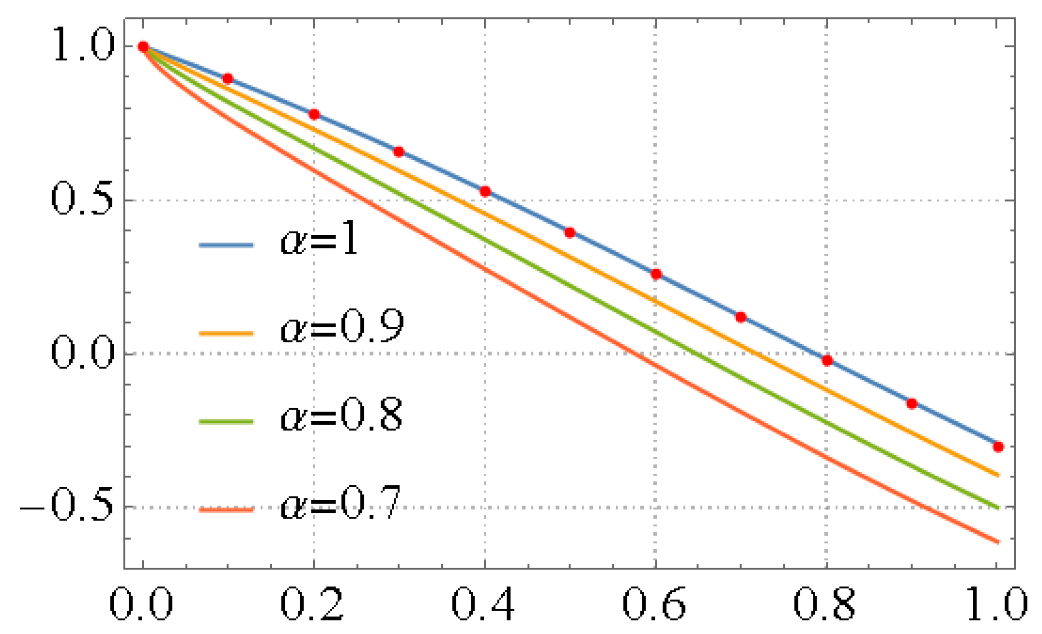
To confirm the accuracy of the recommended approach, we calculate the

R . E .

of the LFPS approximate solution at different numbers of iterations and varied values of fractional order derivative

α

, and summarized in Table 1. One can observe from Table 1 that the numerical comparisons simulation reflects the accuracy of LFPS approach. Graphically, the behavior of attained analytic-approximate series solution of FVIDE (17) is displayed in a 2D plot as in Figure 1. It’s clear that from the graphical representation, the LFPS solutions in different cases of fractional order derivative

α

, simulate the exact solution. Finally, we provided the residual error for Example 1 at different terms and times when fixed value of FD

α = 0.8

. Its clear that, from mentioned simulation in Table 2, the values of residual errors will further decrease via increasing terms. So, the accuracy, efficiency, and convergences of designed algorithm is confirmed.

Example 2.

Consider the following non-linear FVIDE:

D_{t}^{α} u (t) = - 2 \sin (t) - \frac{1}{3} \cos (t) - \frac{2}{3} \cos (2 t) + \int_{0}^{t} \cos (t - x) u^{2} (x) d x, α \in (0,1],

(29)

Subject to the initial condition

u (0) = 1

. The exact solution of (29) at

α = 1

, is

u (t) = \cos (t) - \sin (t)

. [46]

As we do in Example 1, we should be firstly transformed (29) into the new Laplace space; that is:

ξ^{α} U (ξ) - ξ^{α - 1} u (0) = - 2 L [\sin (t)] - \frac{1}{3} L [\cos (t)] - \frac{2}{3} L [\cos (2 t)] + L [\cos (t)] \times L [u^{2} (t)] .

(30)

and the L-REF of (30) can be identified as:

L \{{R e s}_{U} (ξ)\} = U (ξ) - \frac{u (0)}{ξ} - \frac{1}{ξ^{γ q}} (L [\sin (t)] - \frac{1}{3} L [\cos (t)] - \frac{2}{3} L [\cos (2 t)] + L [\cos (t)] \times L [u^{2} (t)]) .

(31)

Write the LTs of (31) in the following FSE:

If $q i$ is odd, then

$L [\sin (t)] = \sum_{i = 0}^{J} \frac{a_{i}}{ξ^{q i + 1}} = \sum_{i = 0}^{J} \frac{{(- 1)}^{\frac{q i - 1}{2}}}{ξ^{q i + 1}},$

(32)
If $q i$ is even, then

$L [\cos (t)] = \sum_{i = 0}^{J} \frac{c_{i}}{ξ^{q i + 1}} = \sum_{i = 0}^{J} \frac{{(- 1)}^{\frac{q i}{2}}}{ξ^{q i + 1}}, L [\cos (2 t)] = \sum_{i = 0}^{J} \frac{b_{i}}{ξ^{q i + 1}} = \sum_{i = 0}^{J} \frac{{(- 1)}^{\frac{q i}{2}} {(2)}^{q i}}{ξ^{q i + 1}},$

(33)
The non-linear term

$L [\cos (t)] \times L [u^{2} (t)] = \sum_{i = 0}^{J} \frac{c_{i}}{ξ^{q i + 1}} \sum_{i = 0}^{2 J} \frac{Γ (q i + 1)}{ξ^{q i + 1}} \sum_{n = \max [0, i - J]}^{\min [J, i]} \frac{u_{n} u_{i - n}}{Γ (n q + 1) Γ (q (i - n) + 1)} = \sum_{i = 0}^{3 J} \frac{1}{ξ^{q (i + \frac{1}{q}) + 1}} \sum_{n = \max [0, i - J]}^{\min [i, 2 J]} Γ (q n + 1) c_{i - n} \sum_{j = \max [0, i - J]}^{\min [J, i]} \frac{u_{j} u_{n - j}}{Γ (q j + 1) Γ (q (n - j) + 1)},$

(34)

Using the FSEs (9, 32-34), the

j

-th L-REF of (32) can be written as:

L \{{R e s}_{U_{J}} (ξ)\} = \sum_{i = 1}^{J} \frac{u_{i}}{ξ^{q i + 1}} + (2 \sum_{i = 0}^{J} \frac{a_{i}}{ξ^{q (i + γ) + 1}} + \frac{1}{3} \sum_{i = 0}^{J} \frac{c_{i}}{ξ^{q (i + γ) + 1}} + \frac{2}{3} \sum_{i = 0}^{J} \frac{b_{i}}{ξ^{q (i + γ) + 1}} - \sum_{i = 0}^{3 J} \frac{1}{ξ^{q (i + \frac{1}{q} + γ) + 1}} \sum_{n = \max [0, i - J]}^{\min [i, 2 J]} Γ (q n + 1) c_{i - n} \sum_{j = \max [0, i - J]}^{\min [J, i]} \frac{u_{j} u_{n - j}}{Γ (q j + 1) Γ (q (n - j) + 1)}) .

(35)

By solving

\underset{ξ \to \infty}{l i m} ξ^{m α + 1} L \{{R e s}_{U_{J}} (ξ)\} = 0

, we have

u_{m} = - (2 a_{m - γ} + \frac{1}{3} c_{m - γ} + \frac{2}{3} b_{m - γ}) + \sum_{n = \max [0, i - J]}^{\min [m - \frac{1}{q} - γ, 2 J]} Γ (q n + 1) c_{m - \frac{1}{q} - γ - n} \sum_{j = \max [0, i - J]}^{\min [J, i]} \frac{u_{j} u_{n - j}}{Γ (q j + 1) Γ (q (n - j) + 1)},

(36)

for

m = γ, γ + 1, \dots, J

, and

u_{0} = 1, u_{i} = 0

for

i = 1,2, \dots, γ - 1 .

In the case of

α = 0.9

, we can choose

q = \frac{1}{10}, γ = 9 .

Setting

u_{0} = 1, u_{i} = 0,

for

i = 1,2, \dots, 8

, then the non-zero terms for

m

from 9 to 40 are

u_{9} = - 1, u_{19} = - 1, u_{28} = - 2, u_{29} = 3, u_{37} = \frac{Γ (\frac{14}{5})}{{Γ (\frac{19}{10})}^{2}}, u_{38} = - 2, u_{39} = 1 .

So, the analytic-approximate solution is given by

u (t) = 1 - \frac{t^{\frac{9}{10}}}{Γ (\frac{19}{10})} - \frac{t^{\frac{19}{10}}}{Γ (\frac{29}{10})} - \frac{2 t^{\frac{14}{5}}}{Γ (\frac{19}{5})} + \frac{3 t^{\frac{29}{10}}}{Γ (\frac{39}{10})} + \frac{t^{\frac{37}{10}} Γ (\frac{14}{5})}{Γ {(\frac{19}{10})}^{2} Γ (\frac{47}{10})} - \frac{2 t^{\frac{19}{5}}}{Γ (\frac{24}{5})} + \frac{t^{\frac{39}{10}}}{Γ (\frac{49}{10})} .

(37)

In the same manner, we gain

γ = 8,7

for

α = 0.8, 0.7

, respectively.

Table 3 compares the residual errors for gained LFPS approximate solutions to FVIDE (29) at varied values of

α

. From Table 3, obvious that the effect of FD parameter on the values of residual errors will further decrease over intrest domain of obtained solutions and this confirms the accuracy of our proposed method. Figure 2 displays the 2D plot of the exact and LFPS solutions for Example 2 when

α \in \{0.7,0.8,0.9,1.0\}

in the domain

t \in [0,1]

. This graphical representation indicates that the attained solutions via recommended algorithm converge to the exact solution when

α

, tends to 1, and these solutions overlap at

α = 1

. Finally, we provided the residual error attained resuts forExample 2 at different terms and times when fixed of FD

α = 0.8

in Table 4 to demonstrate the convergence of the proposed method. From this table, one notice that the values of residual errors will further decrease via increasing terms of obtained solutions, and this proves the accuracy, efficiency, and convergency of LFPS scheme.

5. Conclusions

In this article, a modified LFPS algorithm has been profitably implemented to explore the analytic-approximate solution of non-linear FVIDEs involving the Caputo-FD of order

α : 0 < α \leq 1

, with fitting ICs. The essence and procedure of our recommended algorithm is the construction of the solutions via solving studied equations using LT principle and simulating FPS approach in Laplace space. The accuracy and effectiveness are clarified of LFPS algorithm by graphical and numerical simulations of results. The impact of Caputo-FD order can be observed in the behaviors of LFPS-curves for various values of

α

. Analysis of acquired results declares that the recommended algorithm is considered to be a convenient, reliable computational algorithm to treat wide aspects of non-linear fractional models with high accuracy.

Author Contributions

Conceptualization, A.-K. A. and M. A.; Formal analysis, A.-K. A.; Funding acquisition, M. A. and A.-K. A.; Investigation, M. A., N. T. and A. A.; Methodology, M. A.; Software, A.-K. A.; Supervision, A.-K. A and N. T.; Validation, N. T. and A. A.; Writing – original draft, M. A.; Writing – review & editing, A.-K. A. and N. T. All authors have read and agreed to the published version of the manuscript.

Data Availability Statement

Not applicable.

Conflicts of Interest

The authors declare no conflict of interest.

References

Loverro, A. Fractional calculus: history, definitions and applications for the engineer, Rapport technique, Univeristy of Notre Dame: Department of Aerospace and Mechanical Engineering, 2004.
Mainardi, F. Fractional calculus and waves in linear viscoelasticity: an introduction to mathematical models. World Scientific, 2022.
Yang, X. J. General fractional derivatives: theory, methods and applications. CRC press, 2019.
Kilbas, A. A., Srivastava, H. M., & Trujillo, J. J.” Theory and applications of fractional differential equations”, 2006, 204, elsevier.
Inc, M. Yusuf, A. Aliyu, A. I. and Baleanu, D. Soliton solutions and stability analysis for some conformable nonlinear partial differential equations in mathematical physics, Optical and Quantum Electronics,Volume 50, article 190, 2018. [CrossRef]
Akdemir, A. O., Dutta, H., Atangana, A. “Fractional order analysis: theory, methods and applications”. John Wiley & Sons, 2020.
Bagley R. L. and Torvik, P. J. “Fractional calculus in the transient analysis of viscoelastically damped structures”, AIAA Journal, 1985, 23(6), 918–925, 1985. [CrossRef]
Al-Smadi, M.; Djeddi, N.; Momani, S. Al-Omari, S; Araci, S. “An attractive numerical algorithm for solving nonlinear Caputo–Fabrizio fractional Abel differential equation in a Hilbert space”, Advances in Difference Equations, Volume 2021, Article ID 271, 2021. [CrossRef]
Ragb, O. Wazwaz, A. M. Mohamed, M. Matbuly, M. S. Salah, M. “Fractional differential quadrature techniques for fractional order Cauchy reaction--diffusion equations”. Mathematical Methods in the Applied Sciences, 2023. [CrossRef]
Hashim, I.; Sharadga, M.; Syam, M.I.; Al-Refai, M. A Reliable Approach for Solving Delay Fractional Differential Equations. Fractal Fract. 2022, 6, 124. [CrossRef]
Bataineh M.; Alaroud M, Al-Omari S, Agarwal P. “Series Representations for Uncertain Fractional IVPs in the Fuzzy Conformable Fractional Sense”. Entropy. 2021; 23(12):1646. [CrossRef]
Syam, M.; Al-Refai, M. “First order delay equations Implicit hybrid method”. Alex. Eng. J. 2020, 59, 2677–2681.
Al-qudah, Y.; Alaroud, M.; Qoqazeh, H.; Jaradat, A.; Alhazmi, S.E.; Al-Omari, S. Approximate Analytic–Numeric Fuzzy Solutions of Fuzzy Fractional Equations Using a Residual Power Series Approach. Symmetry 2022, 14, 804. [CrossRef]
Hengamian Asl, E., Saberi-Nadjafi, J., Gachpazan, M. “Numerical Solution of Fractional-Order Population Growth Model Using Fractional-Order Muntz–Legender Collocation Method and Pade–Approximations”, Jordan Journal of Mathematics and Statistics, (2022),15.
Hartley,T. T., Lorenzo, C. F. and Killory Qammer, H. “Chaos in a fractional order Chua's system”, IEEE Transactions on Circuits and Systems I: Fundamental Theory and Applications, 1995, 42(8), 485–490.
Oldham, K. B. “The reformulation of an infinite sum via semiintegration”, SIAM Journal on Mathematical Analysis, 1983, 14, (5), 974–981.
Povstenko, Y. Z, “Thermoelasticity that uses fractional heat conduction equation”, Journal of Mathematical Sciences, 2009, 162 (2), 296–305.
Baskin, E. and Iomin, A. Electro-chemical manifestation of nanoplasmonics in fractal media, Central European Journal of Physics, 2013, 11(6), 676–684.
Bapna, I. B. and Mathur, N. Application of fractional calculus in statistics, International Journal of Contemporary Mathematical Sciences, 2012, 7(17-20), 849–856.
Goncalves E. and Zeidan,D, “Numerical simulation of unsteady cavitation in liquid hydrogen flows”, Journal of Engineering Systems Modelling and Simulation, 2017, 9(1)pp. 41–51, 2017.
Kulish V. V. and Lage, J. L, “Application of fractional calculus to fluid mechanics”, Journal of Fluids Engineering, 2002, 124, (3), 803–806.
Derdar, N. “Nonlinear Implicit Caputo-Hadamard Fractional Differential Equation with Fractional Boundary Conditions”. Jordan Journal of Mathematics and Statistics (JJMS), 2022, 15(4B), 999-1014.
Bendouma, B. “Monotone Iterative Technique for a Coupled System of Nonlinear Conformable Fractional Dynamic Equations on Time Scales”. Jordan J. Math. Stat. JJMS, 2023, 16, 41–55.
Al-Smadi, M., Al-Omari, S., Karaca, Y., and Momani, S. Effective Analytical Computational Technique for Conformable Time-Fractional Nonlinear Gardner Equation and Cahn-Hilliard Equations of Fourth and Sixth Order Emerging in Dispersive Media, Journal of Function Spaces, 2022.
Alaroud, M.; Alomari, A.-K.; Tahat, N.; Al-Omari, S.; Ishak, A. “A Novel Solution Approach for Time-Fractional Hyperbolic Telegraph Differential Equation with Caputo Time Differentiation”. Mathematics 2023, 11, 2181. [CrossRef]
Alaroud, M.; Al-Smadi, M.; Rozita Ahmad, R.; Salma Din, U.K. “An Analytical Numerical Method for Solving Fuzzy Fractional Volterra Integro-Differential Equations”. Symmetry 2019, 11, 205. [CrossRef]
Ma, C. “A Novel Computational Technique for Impulsive Fractional Differential Equations”. Symmetry 2019, 11, 216. [CrossRef]
Mahmood, S.; Shah, R.; khan, H.; Arif, M. “Laplace Adomian Decomposition Method for Multi Dimensional Time Fractional Model of Navier-Stokes Equation. Symmetry 2019, 11, 149. [CrossRef]
Youbi, F.; Momani, S.; Hasan, S.; Al-Smadi, M. “Effective numerical technique for nonlinear Caputo-Fabrizio systems of fractional Volterra integro-differential equations in Hilbert space”. Alex. Eng. J. 61(3), 1778-1786, 2022.
Zedan, H. A.; Alaidarous, E., “Haar wavelet method for the system of integral equations”, Abstract and Applied Analysis, vol. 2014, Article ID 418909, 9 pages, 2014.
Biazar, J. “Solution of systems of integral-differential equations by Adomian decomposition method”, Applied Mathematics and Computation, vol. 168, no. 2, pp. 1232–1238, 2005.
S. Abbasbandy, M. S. Hashemi, and I. Hashim, “On convergence of homotopy analysis method and its application to fractional integro-differential equations”, Quaestiones Mathematicae, vol. 36, no. 1, pp. 93–105, 2013.
D. Baleanu, S. Zibaei, M. Namjoo, and A. Jajarmi, “A nonstandard finite difference scheme for the modeling and non-identical synchronization of a novel fractional chaotic system”, Advances in Difference Equations, vol. 2021, no. 1, pp. 1–19, 2021.
K. Maleknejad, N. Aghazadeh, and M. Rabbani, Numerical solution of second kind Fredholm integral equations system by using a Taylor-series expansion method, Applied Mathematics and Computation, vol. 175, no. 2, pp. 1229–1234, 2006.
N. Sahin, S. Yuzbasi, and M. Gulsu, A collocation approach for solving systems of linear Volterra integral equations with variable coefficients, Computers & Mathematics with Applications, vol. 62, no. 2, pp. 755–769, 2011.
M. Alaroud, M. Al-smadi, R. R. Ahmad, and U. K. S. Din, “Numerical computation of fractional Fredholm integro-differential equation of order 2β arising in natural sciences”. In Journal of Physics: Conference Series (Vol. 1212, No. 1, p. 012022). IOP Publishing, (2019, April).
H. Aljarrah, M. Alaroud, A. Ishak, M. Darus, “Adaptation of Residual-Error Series Algorithm to Handle Fractional System of Partial Differential Equations”. Mathematics 2021, 9, 2868. [CrossRef]
M. A. Hammad, M. Alaroud, O. A. Arqub, R. Edwan, M. Al-Smadi and S. Momani, “Solving Fuzzy Fractional IVPs of order 2β by Residual Power Series Algorithm”, 2019 IEEE Jordan International Joint Conference on Electrical Engineering and Information Technology (JEEIT), Amman, Jordan, 2019, pp. 52–57. [CrossRef]
M. I. Liaqat, A. Khan, M. Alam, and M. K. Pandit, “A highly accurate technique to obtain exact solutions to time-fractional quantum mechanics problems with zero and nonzero trapping potential”, Journal of Mathematics, vol. 2022, Article ID 9999070, 20 pages, 2022.
Alaroud, M., Tahat, N., Al-Omari, S., Suthar, D. L., & Gulyaz-Ozyurt, S. , “An Attractive Approach Associated with Transform Functions for Solving Certain Fractional Swift-Hohenberg Equation”, Journal of Function Spaces, vol. 2021, Article ID 3230272, 14 pages, 2021. [CrossRef]
Liaqat, M. I., and Okyere, E. “Comparative Analysis of the Time-Fractional Black–Scholes Option Pricing Equations (BSOPE) by the Laplace Residual Power Series Method (LRPSM)”. Journal of Mathematics, 2023.
Aljarrah, H.; Alaroud, M.; Ishak, A.; Darus, M. Approximate Solution of Nonlinear Time-Fractional PDEs by Laplace Residual Power Series Method. Mathematics 2022, 10, 1980. [CrossRef]
Alaroud, M.; Ababneh, O.; Tahat, N.; Al-Omari, S. “Analytic technique for solving temporal time-fractional gas dynamics equations with Caputo fractional derivative”. AIMS Math 2022, 7, 17647–17669.
Alaroud, M.; Alomari, A.-K.; Tahat, N.; Ishak, A. “Analytical Computational Scheme for Multivariate Nonlinear Time-Fractional Generalized Biological Population Model”. Fractal Fract. 2023, 7, 176. [CrossRef]
Oqielat, M.A.N.; Eriqat, T.; Al-Zhour, Z.; Ogilat, O.; El-Ajou, A.; Hashim, I. “Construction of fractional series solutions to nonlinear fractional reaction–diffusion for bacteria growth model via Laplace residual power series method”. Int. J. Dyn. Control 2023, 11, 520–527.
Wazwaz, A. M. “The combined Laplace transform–Adomian decomposition method for handling nonlinear Volterra integro–differential equations. Applied Mathematics and Computation”, 2010), 216(4), 1304-1309.
Moa’ath, N. O., El-Ajou, A., Al-Zhour, Z., Eriqat, T., and Al-Smadi, M. A new approach to solving fuzzy quadratic Riccati differential equations. International Journal of Fuzzy Logic and Intelligent Systems, 2022, 22(1), 23-47.

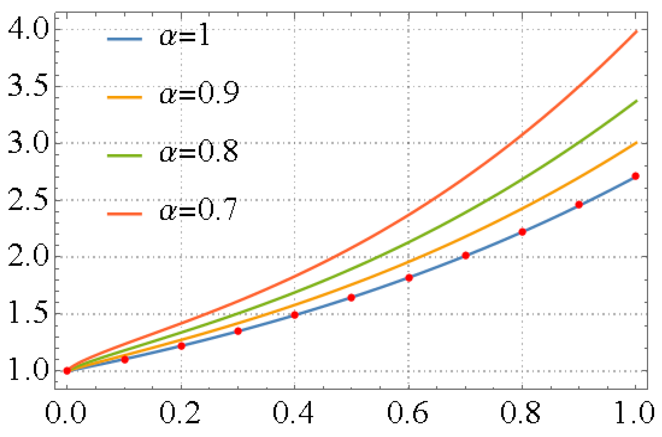
Figure 1. 2D plots of fractional curves of the LFPS approximate solution for Example 1, at various values of

α

, versus the exact solution.

Figure 1. 2D plots of fractional curves of the LFPS approximate solution for Example 1, at various values of

α

, versus the exact solution.

Figure 2. 2D plots of fractional curves of the LFPS approximate solution for Example 2 at various values of

α

, versus the exact solution.

Figure 2. 2D plots of fractional curves of the LFPS approximate solution for Example 2 at various values of

α

, versus the exact solution.

Table 1. The residual error of the LFPS solutions for Example 1.

$t_{i}$	$α = 0.9$	$α = 0.8$	$α = 0.7$	$α = 0.6$
$0.1$	$3.05125 \times 10^{- 8}$	$2.76818 \times 10^{- 8}$	$1.25598 \times 10^{- 7}$	$3.32936 \times 10^{- 7}$
$0.2$	$5.44445 \times 10^{- 6}$	$2.4180 \times 10^{- 6}$	$2.70504 \times 10^{- 5}$	$7.78659 \times 10^{- 5}$
$0.3$	$1.15718 \times 10^{- 4}$	$1.38234 \times 10^{- 6}$	$6.74897 \times 10^{- 4}$	$2.07896 \times 10^{- 3}$
$0.4$	$1.03751 \times 10^{- 3}$	$4.43181 \times 10^{- 4}$	$7.01985 \times 10^{- 3}$	$2.28483 \times 10^{- 2}$

Table 2. The residual error of the LFPS solutions at different terms and times with

α = 0.8

for Example 1.

Table 2. The residual error of the LFPS solutions at different terms and times with

α = 0.8

for Example 1.

	$J$	20	40	60	80
$t_{i}$		20	40	60	80
0.1		$2.23231 \times 10^{- 2}$	$6.03273 \times 10^{- 4}$	$5.48087 \times 10^{- 6}$	$2.76818 \times 10^{- 8}$
0.2		$8.31149 \times 10^{- 2}$	$7.32976 \times 10^{- 3}$	$2.58114 \times 10^{- 4}$	$2.4180 \times 10^{- 6}$
0.3		$1.85919 \times 10^{- 1}$	$3.28381 \times 10^{- 2}$	$2.64048 \times 10^{- 3}$	$1.38234 \times 10^{- 6}$
0.4		$3.35873 \times 10^{- 1}$	$9.8273 \times 10^{- 2}$	$1.45347 \times 10^{- 2}$	$4.43181 \times 10^{- 4}$

Table 3. The residual error of the LFPS solutions for Example 2.

$t_{i}$	$α = 0.9$	$α = 0.8$	$α = 0.7$	$α = 0.6$	$α = 0.5$
$0.1$	$4.01872 \times 10^{- 12}$	$1.14969 \times 10^{- 10}$	$3.51448 \times 10^{- 11}$	$1.2662 \times 10^{- 10}$	$7.2709 \times 10^{- 11}$
$0.2$	$8.73393 \times 10^{- 10}$	$3.65742 \times 10^{- 8}$	$1.19959 \times 10^{- 8}$	$3.75249 \times 10^{- 8}$	$2.55736 \times 10^{- 8}$
$0.3$	$1.60784 \times 10^{- 8}$	$1.06161 \times 10^{- 6}$	$3.56381 \times 10^{- 7}$	$9.78584 \times 10^{- 7}$	$6.88552 \times 10^{- 7}$
$0.4$	$8.94261 \times 10^{- 8}$	$1.15723 \times 10^{- 5}$	$3.91616 \times 10^{- 6}$	$9.47861 \times 10^{- 6}$	$6.18322 \times 10^{- 6}$
$0.5$	$9.02043 \times 10^{- 8}$	$7.37875 \times 10^{- 5}$	$2.49509 \times 10^{- 5}$	$5.35762 \times 10^{- 5}$	$2.78115 \times 10^{- 5}$

Table 4. The residual error of the LFPS solutions at different terms and times with

α = 0.8

for Example 2.

Table 4. The residual error of the LFPS solutions at different terms and times with

α = 0.8

for Example 2.

	20	40	60	80
$t_{i}$	20	40	60	80
0.1	$3.23928 \times 10^{- 3}$	$4.56363 \times 10^{- 5}$	$3.98756 \times 10^{- 7}$	$2.06271 \times 10^{- 9}$
0.2	$1.81809 \times 10^{- 3}$	$5.3666 \times 10^{- 4}$	$1.43983 \times 10^{- 5}$	$3.32608 \times 10^{- 7}$
0.3	$1.00238 \times 10^{- 2}$	$2.20152 \times 10^{- 3}$	$1.13732 \times 10^{- 4}$	$6.45179 \times 10^{- 6}$
0.4	$3.55286 \times 10^{- 2}$	$5.84874 \times 10^{- 3}$	$4.83321 \times 10^{- 4}$	$5.2582 \times 10^{- 5}$

Disclaimer/Publisher’s Note: The statements, opinions and data contained in all publications are solely those of the individual author(s) and contributor(s) and not of MDPI and/or the editor(s). MDPI and/or the editor(s) disclaim responsibility for any injury to people or property resulting from any ideas, methods, instructions or products referred to in the content.

© 2023 by the authors. Licensee MDPI, Basel, Switzerland. This article is an open access article distributed under the terms and conditions of the Creative Commons Attribution (CC BY) license (http://creativecommons.org/licenses/by/4.0/).

Copyright: This open access article is published under a Creative Commons CC BY 4.0 license, which permit the free download, distribution, and reuse, provided that the author and preprint are cited in any reuse.

MDPI Initiatives

Important Links

Choose an area of interest and we will send you notifications of new preprints at your preferred frequency.

Disclaimer

Extended Laplace Power Series Method for Solving Non-linear Caputo Fractional Volterra Integro-differential Equations

Abstract

1. Introduction

2. Preliminaries and Basic Concepts

3. Principle of the LFPS Algorithm

4. Illustrated Examples

5. Conclusions

Author Contributions

Data Availability Statement

Conflicts of Interest

References

MDPI Initiatives

Important Links

Subscribe