1. Introduction
It has been more than two years since Covid-19 was declared as a global pandemic on March 11, 2020 by the World Health Organization (WHO). According to the WHO, the respiratory syndrome Coronavirus 2 (SARS-CoV-2) which was first encountered in December 2019 [
1] in Wuhan District of China has caused 629, 370, 889 confirmed cases and 6, 578, 245 deaths as of November 7, 2022. To preclude the spread of the of Covid-19, governing bodies of cities, states and countries have adapted various non-pharmaceutical and pharmaceutical interventions [
1]. Though, most of the attempts have proven to be effective in controlling the pandemic it has affected the economic and social welfare in numerous ways.
Statista, a German company specializing in market and consumer data states that the world experienced a drop of 3.4% in Gross Domestic Product (GDP) and a 6.57% increment in global unemployment rate in the year 2020. Furthermore, this has affected the lives of human beings causing degradation in mental health [
2], changes in behavior [
1], malnutrition due lack of food security [
3], etc.
Most of the above-mentioned circumstances could have been avoided or mitigated if the governments were able to impose the interventions in a much more effective manner by considering the balance between socio-economic impact and disease propagation. In addition, these decisions should be made at a more granular manner as opposed to sweeping brute force approaches that were performed mostly based on assumptions. Some countries experienced consecutive waves of an outbreak due to mismanagement of containment strategies put forth by the governments [
4]. Imposing and lifting off lockdowns, the stay-at-home orders, travel restrictions, quarantine measures, and bans on gathering events at the optimum time has a major impact on preventing further spread of the disease.
The Sustainable Development Goals (SDGs) set forward by United Nations (UN), contain the requirement of having sustainable cities and societies which are inclusive, safe, resilient and sustainable. This requires the reduction of deaths and the number of people affected by natural disasters while decreasing direct economic losses. Furthermore, it attempts to ensure that the human settlements are adopting and implementing plans towards inclusion, mitigation, adaption and resilience to disasters in order to develop risk reduction strategies.
In the face of a pandemic like Covid-19, it is vital to understand the interrelationships among transmission mechanics with each mutation, subtle behavior changes, social interactions during each surge, the impact of numerous containment measures at different administrative levels and, the penetration of vaccinations to build up the resilience towards communicable diseases and make the city, state or country sustainable.
Furthermore, discovering the vulnerable locations and, an occupation-based vulnerability assessment will assist the health care officials to identify the disease spread hot-spots in the communities. Which in turn supports more precise and pinpoint containment, resource allocation and, policy implication. As occupation is a decisive factor in deciding their daily routine as well as the inclination of being a victim of risks (e.g., health sector employees are highly susceptible because they work closely with infected patients), it is necessary to fathom and foresee the relative susceptibility towards the disease for each occupation and, how an infection cluster might propagate through professions and locations based on the origin or source of infection.
1.1. Contribution
In PDSIM, we introduce a more robust approach to modeling the complex movement dynamics of the population while considering individuals’ occupations. We provide a User Interface that allows for the creation of more realistic environments and incorporates behaviour modeling techniques. Additionally, PDSIM enables the conversion of a person’s experiences, expressed through a language, into a probabilistic model, enhancing the ability to accurately represent real-world scenarios.
The behaviour of a population is commonly modeled using Agent-Based Models (ABMs). In ABMs, the random walk has been widely utilized as a simple form of mobility [
5]. However, when analyzing a person’s movement at a macroscopic level, it does not exhibit the characteristics of a truly random or pseudo-random walk. Instead, it follows a hybrid mechanism where individuals make macroscopic-level decisions regarding their next target location before moving, while concurrently exhibiting more random-like movements within specific locations. In order to capture this behavior, PDSIM employs a combination of random walk within specific locations and, discrete state transitions based on decision-making for movement between locations.
Additionally, the proposed simulator allows the customization of the probability distributions of each occupation class which are related to the decision-making process mentioned above. The probability matrices are tuned accommodating the specific behavior patterns of occupation classes. Tuning of the parameters can be done from the data extracted through a survey, that conducted on the behavior patterns of people in the region of interest.
When modeling the disease propagation dynamics it is crucial to consider the mode of transportation used by the agents. To build a resilient and sustainable transport system and to rebuild trust in public transport [
6], it is important to understand the role of mobility amidst a pandemic such as Covid-19. Eventhough, [
7,
8,
9] use scenarios that were based on complex intervention strategies, they miss the important interactions that occur when the agents use different movement methods, specially public transportation systems. PDSIM has been designed to incorporate the micro-level interactions occurring within public places, work places, transportation networks and events, subjected to the level of social distance practiced. This enables the assessment of the impact of human behavior at a granular level on disease propagation.
PDSIM can serve as a valuable tool for simulating various containment strategies, exploring spread of the disease and its impact on the society, thereby enabling policymakers to make well-informed decisions of when and how the strategies should be imposed. A summary of the major contributions of PDSIM is given below,
A hybrid movement model with realistic motion simulation incorporating real human-like behavior and decision making for inter and intra-location movement.
Occupation-specific motion and daily routine generation through the "daily routine generator" of simulation engine, based on probabilistic models that are tuned at occupation level. A unique and easily tune-able probabilistic function to derive the agent motion pattern based on their occupation characteristics.
A novel location occupancy mechanic to determine how long someone stays at a given location prior to location state transition determines the next target location. This mechanism stabilizes the location state transition by allowing it to trigger only when a decision to leave is taken thus injecting a more human like decision making process to the motion model.
An environment generator that uses a tree structure to build diverse surroundings which are highly scaleable and adaptable such that it enables the user to develop urban or other environments based on demographics and focus (manufactural, commercial, residential, etc ). In addition, zones have been added to the environment, substantially simplifying it while maintaining a realistic emulation impact evaluation.
Incorporation of public and private transport systems in to the simulation environment enabling the ability simulate the impact of public transport in disease propagation.
Ability to simulate Super-Spreader events (Large gatherings), testing and vaccination protocols, social distancing and hygiene (mask-wearing and sanitizing) of people, multiple types of containment policies and assess their impact on disease propagation.
Ability to design detailed variants, different communicable diseases, environment, and people (age factors, immunity, hygiene, etc.) based disease transmission models.
2. A Brief Review on Epidemic Models
The potential to gain insights into the dynamics of infectious diseases and their impact on the population has made mathematical modeling a critical tool in epidemiology [
10,
11]. By systematically representing reported cases and deaths through historical data replication, mathematical modeling helps predict the number of infected patients and, identifies long-term disease spread behavior. This allows policymakers to prepare for worst-case scenarios and implement strategies for disease prevention while considering the social and economic well-being of the population.
The available mathematical models for pandemic simulation can be classified into two main types: Compartment Models and Agent-Based Models (ABMs). The most commonly used simple compartment models divide the population into compartments representing different states. These compartments are often assigned to
Susceptible,
Infected, and
Recovered (SIR) statistics, while dynamics between them are modeled using differential equations [
12]. Although the use of compartment models to simulate epidemics initiated with [
13], they have evolved significantly through the introduction of more detailed compartments and conditions to analyze the dynamics more comprehensively [
14]. The SIR models have been further expanded to include SEIR and SEQIR models, which incorporate compartments for the Exposed and Quarantined population [
13,
15]. Improvements on the classical epidemic SEIR models have been made through the incorporation of Multistage Time-delay Control Models (MTCM) for Covid-19 transmission, resulting in better simulation results [
16]. Furthermore, [
6] incorporates an activity-based transport model to simulate the spread of the disease on a regional scale. These models have been used to evaluate the efficacy of contact tracing [
17] and other interventions, ensuring the sustainability of communities against pandemic scenarios [
6,
18].
Compared to compartment models, Agent-Based Models (ABMs) offer a more detailed approach to modeling the population with individual attention to each agent. ABMs are advantageous in investigating individual behaviour and the spread of diseases as well as capturing variations in demographic, social, and economic elements within a population [
19]. ABMs have been used to simulate the spread of infectious diseases in various environments, ranging from workplaces and households to large cities, under different control strategies [
7]. Several agent-based influenza pandemic models have been repurposed to simulate the spread of Covid-19 transmission and the impact of social distancing measures in different countries [
20,
21]. Moreover, new ABMs have been developed to evaluate the impact of social distancing, contact tracing [
22,
23], and super-spreading events [
24].
PDSIM is a comprehensive and versatile model, distinguishing it from alternative models presented in the literature. The unique features of the proposed architecture compared to the existing simulation models are presented in
Table 1. Most models in the literature focus on analyzing specific aspects of a pandemic, such as disease propagation [
25], intervention effectiveness [
26] and, transportation [
6,
27,
28]. However, PDSIM takes a multi-dimensional approach, accounting for numerous key variables associated with pandemic spread. PDSIM includes features such as disease propagation modeling, hygiene simulation, recreational activities, testing protocols, vaccination and, containment strategies, which are common to the prior models. It also introduces novel features, such as generative realistic human motion, public transportation systems, unique and detailed daily routines, and super-spreader events, which are critical in analyzing pandemic behaviour.
Moreover, the ability of PDSIM to easily calibrate the motion model and construct an environment to match the demographics and dynamics of a specific region of interest makes it a versatile tool compared to other replicator models that require a vast database of real data specific to the environment being simulated. This integrated model is extremely useful for decision-makers who must balance multiple priorities and objectives in response to a pandemic. Additionally, a tool with this potential can identify pandemic preparedness and the effectiveness of the policymakers’ response, providing insight into more effective decision-making to enhance the community’s sustainability against future pandemics.
3. Materials and Methods
PDSIM is an Agent-Based Model where an agent represents a person in a community that is divided into occupational categories. The movement patterns of each agent are mainly driven by their occupational class. During the simulation, each agent will follow a unique trajectory shaped by the occupation of the individual. Furthermore, PDSIM is capable of simulating the disease transmission between agents concurrently, accounting for the disease progression inside the body of an infected agent until recovery or death. The agents are modeled to respond to factors such as time, disease infection, lockdown/quarantine measures and public events.
The PDSIM provides the flexibility to adjust parameters through an interface to tune the simulator in-order to mimic different real-world environments with their inherent features. These parameters will directly affect the simulation by varying intrinsic properties of agents, locations, and movement methods. In addition, the capability to adjust disease-related parameters allows the user to analyse the effect of different variants and their effect on disease spread.
The following sections will include an in-depth discussion on the modeling of the PDSIM. The initial section will focus on how COVID-19 disease propagation is modeled in the simulator and, the mechanisms used to model the transmission of the disease. Afterwards, the modeling of the environment and people will be discussed including the modeling of mobility for agents based on factors such as occupation, the state of the day and containment strategies imposed by the governing bodies. Then, in the Interventions section, the tools that can be used to do experiments with the simulator, where the user can change the social distancing protocols, hygiene practices enforced in different locations, testing protocols, vaccination strategies, isolated areas and, various social events are presented. Next, an illustration of the additional features included in PDSIM where users can easily calibrate and run simulations while visualizing and interpreting the outputs using an intuitive UI is included.
3.1. Disease Propagation
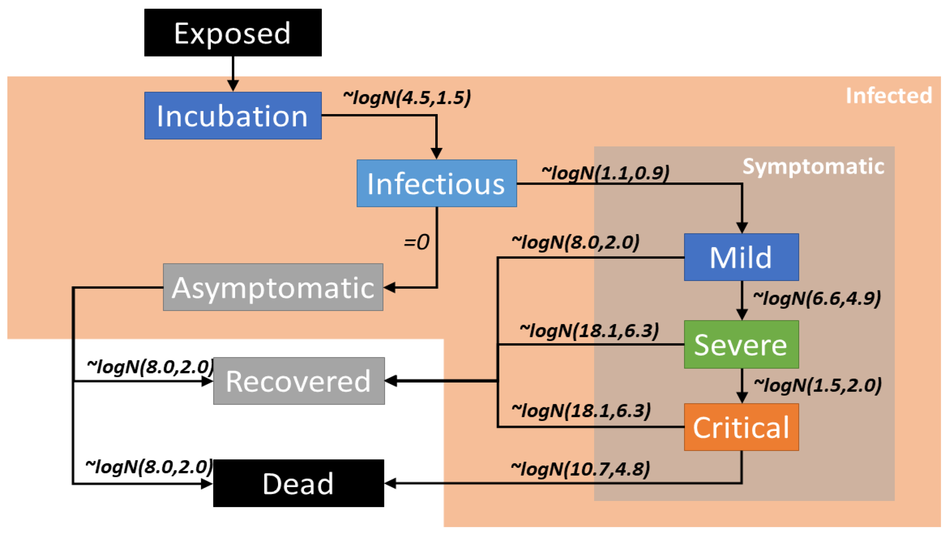
The population was separated into different categories which represent the disease state, namely Susceptible, Infected, Recovered, and Dead. Depending on the indications of symptoms the Infected category was further divided into Asymptomatic and Symptomatic states. The progression from one state to another is illustrated in
Figure 1. The Symptomatic state is separated into Mild, Severe, and Critical stages (
) to evaluate the severity of the infection. The probability values for progression from each state and each age group is given in
Table 2.
The PDSIM provides the flexibility to adjust parameters such as incubation period, the ratio of asymptomatic agents from all infected agents and, the probability functions related to disease severity, allowing the user to introduce and analyse the behaviour of existing and potential variants. This could eventually assist the health care providers and the governing bodies of the city/country to impose containment strategies to effectively control the spread of the disease. Furthermore, PDSIM can also be used to assess the impact of different types of pandemics and disease variants to identify the classes or communities which need more assistance and protection to plan accordingly while building-up resilience.
3.2. Transmission of Disease
Current studies have proven that the transmission of Covid-19 can happen just before developing symptoms as well as when symptoms are visible, given that the people were in contact for a prolonged period. Even though asymptomatic agents are capable of transmitting the disease, the relative transmissibility of asymptomatic patients is lower compared to symptomatic patients. To mimic the less likelihood of getting in contact with infectious aerosols from an infected individual a decaying function is used as the transmission probability variation with distance. The simulator provides the flexibility of introducing new variants of Covid-19 allowing the user to adjust parameters such as transmissibility, infectability and the transmission probability variation with distance.
3.3. Environment Structure
In order to test the effectiveness of the containment strategies on an environment using a simulation model, the virtual model of the environment should represent the infrastructure of the actual environment, up to some extent. However, depending on the type of environment, the locations which needed to be included can vary. Modeling all these locations for different environments is a tedious task. Therefore, PDSIM has pre-built locations separated into several classes that can be used to model complex environments by defining the location details and connecting these locations using a hierarchical structure.
3.3.1. Locations and Functionality
A location is defined as a land area with a boundary and performs as a specific place essential for an agent to follow their daily routine. A location can overlap another location (i.e., land areas are not mutually exclusive), and a location does not change its’ shape with time. In PDSIM, a circle or polygon represents a location. Different types of locations are modeled in PDSIM such as “Homes”, “Hospitals”, “Parks”, “Residential Zones”, etc.
3.3.2. Hierarchical Modeling of the Environment/World Using Locations
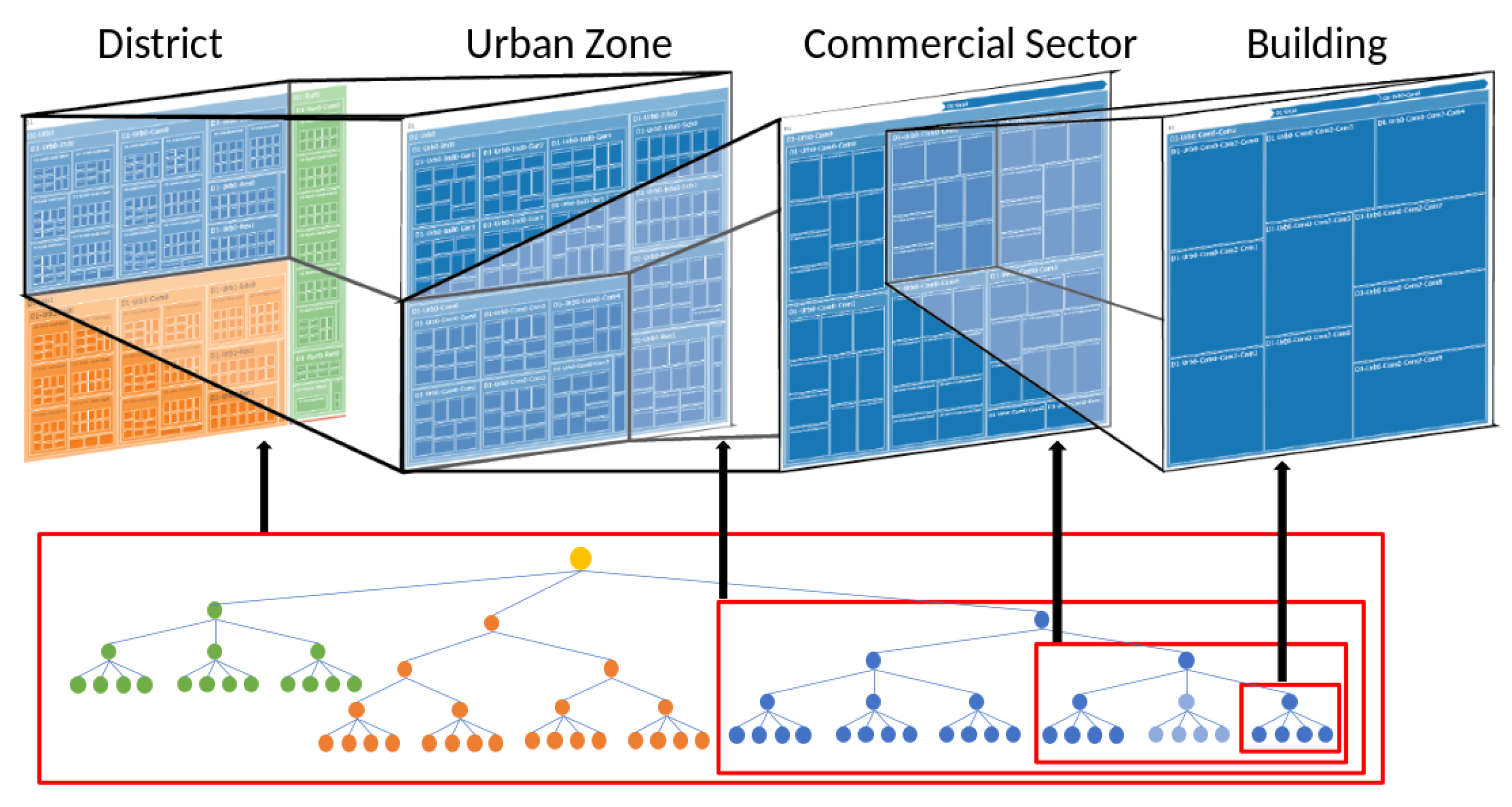
The tree structure used to model the environment is shown in
Figure 2. The structuring is done in such a way that it realizes agent movement in the best method as a tree traversal. If an agent is travelling from the house to a shop in the town, then, he/she must leave the node corresponding to the house and enter the residential zone. Next, the agent has to travel to the network representing the city prior to entering the desired building.
Furthermore, this tree structure provides the flexibility to design different environments by adding and removing blocks. The district illustrated in
Figure 2 consists of two urban towns and a single rural town depicted using different colour schemes. The rural setting does not contain many sub-sections, while the urban setting contains many sectors such as garment sectors, commercial sectors, and residential sectors that further detail the structure of the urban town. The selected commercial sector is made out using six buildings. A building is constructed as a collection of diverse rooms which is considered as the basic building block of the environment. Once an environment is built it can be used as a building block to build a much larger environment. This structure further simplifies the modeling of the environment of interest, while preserving the realistic nature to successfully simulate the impact assessment on a given location.
3.4. Agents
An agent in PDSIM represents one person in the real world. To predict and investigate the disease’s spread, accurate modeling of human mobility is required. In the real world, the mobility of people is greatly shaped by their occupation. Owing to this fact the agents are categorized depending on the occupation category/functionality in society. Different agent classes such as commercial workers, hospital workers, administrative officials, students, elderly citizens, etc. are presented in PDSIM allowing users to customize the population as needed.
An agent class has properties like age and gender that can be initialized at the start, to represent the demographics of a given region. Each agent is assigned a location modeled as a home and working place for the entirety of the simulation. In a high-level picture, an agent should go to the working place in the morning from home and come back home in the evening on weekdays, and they won’t return to the working place on the weekends. If a simple daily routine for each agent is initialized, then agents in the same class will have similar routines. This repetition is avoided by assigning each agent to different working places and homes. Further, the routes are perturbed by various daily chores that people are doing. For example, some people visit supermarkets when returning home from the workplace or visit the hospital, school, markets, etc. The set of locations an agent visits in a daily routine is determined through a discrete pseudo-random sequence generated based on an agent’s probability of being at a given location at a given time. This helps in achieving more individualized randomness among agents of the same class.
Moreover, an agent has other fuzzy parameters like immunity, body temperature, hygienic behaviour and, social and physical characteristics, which are used for the disease simulation and daily routine adjustments to promote uniqueness further. When an agent gets infected, the information about the source of infection, infected place, and time will be logged to analyze the disease’s spread. Also, the test result is stored in the agent if an agent was tested for Covid-19 using a given testing procedure. Also, the position at each time step, locations that they travelled, movement methods used and, close contacts at each time step will be stored for further analysis.
3.5. Mobility
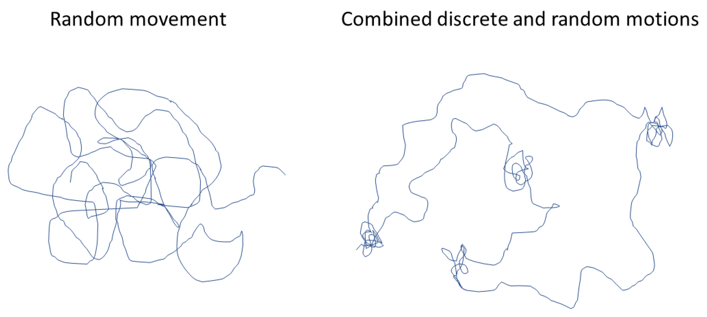
It is imperative to make sure that the movement of the agents in PDSIM resembles the real-world motion of people. Usually, movement is modeled as a random variation of the position in 2D space. But in the real world, most people move in a combined discrete and random fashion which is illustrated in
Figure 3. The discrete movement is a result of moving between different locations.
In PDSIM several strategies are used for moving agents according to the aforementioned combined discrete and random motion. At the beginning of a given day, a daily routine for each agent will be initialized based on the day of the week and the type of containment policies applied on that day. For example, a person of a particular occupation changes their daily routine if a lockdown measure is applied to the population on the weekend. As people decide on the location to visit beforehand the movement, in between locations movement is adapted to be discrete. On the contrary, the in-location movement of a human is dependent on the sudden decision. Hence, it is modeled to be a random motion.
The following sections are dedicated to elucidating the methodologies used for daily routine initialization, unique mobility pattern generation and, describing the movement systems used in PDSIM.
3.5.1. Daily Routes Initialization
At the beginning of the day, each agent should decide which locations they should visit throughout the day. Next, arrange them in a discrete sequence as the agent’s daily routine. The goal of the simulator is to move the agent from the starting location to the end location passing through all intermediate locations of the sequence. This route contains locations that the agent should visit and a corresponding leaving time for each location. If an agent visits a particular place, the agent should stay there until the leaving time following a specific movement pattern. When it is time to leave the location, the agent will use a preferred movement system for moving to the next location.
Building the daily routine for an agent according to the aforementioned method gives arise to two central problems:
To solve these problems, two probability matrices are introduced. These matrices are used to decide an agent’s tendency to visit a particular location at a given time (visit-probability matrix ) and how long that agent will stay at that location (occupancy-probability matrix ).
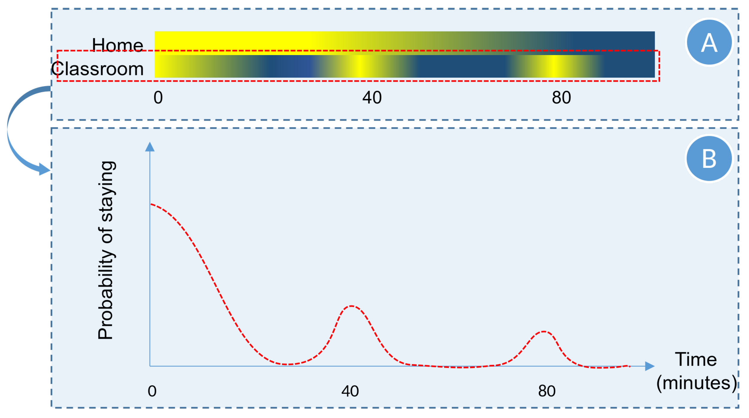
The probability of going to a particular location at a given time of a day is provided by the Location visit-probability matrix . Each agent class (based on their occupation) has a unique matrix where is the number of different types of locations, and 1440 is the number of minutes in a day. To understand how the simulator selects a location using the , let us consider two location types (at ) “Home” and “Classroom”.
When initializing the daily routine, to decide where an agent would be at time
t, PDSIM extracts the visit probabilities of all potential locations for an agent based on
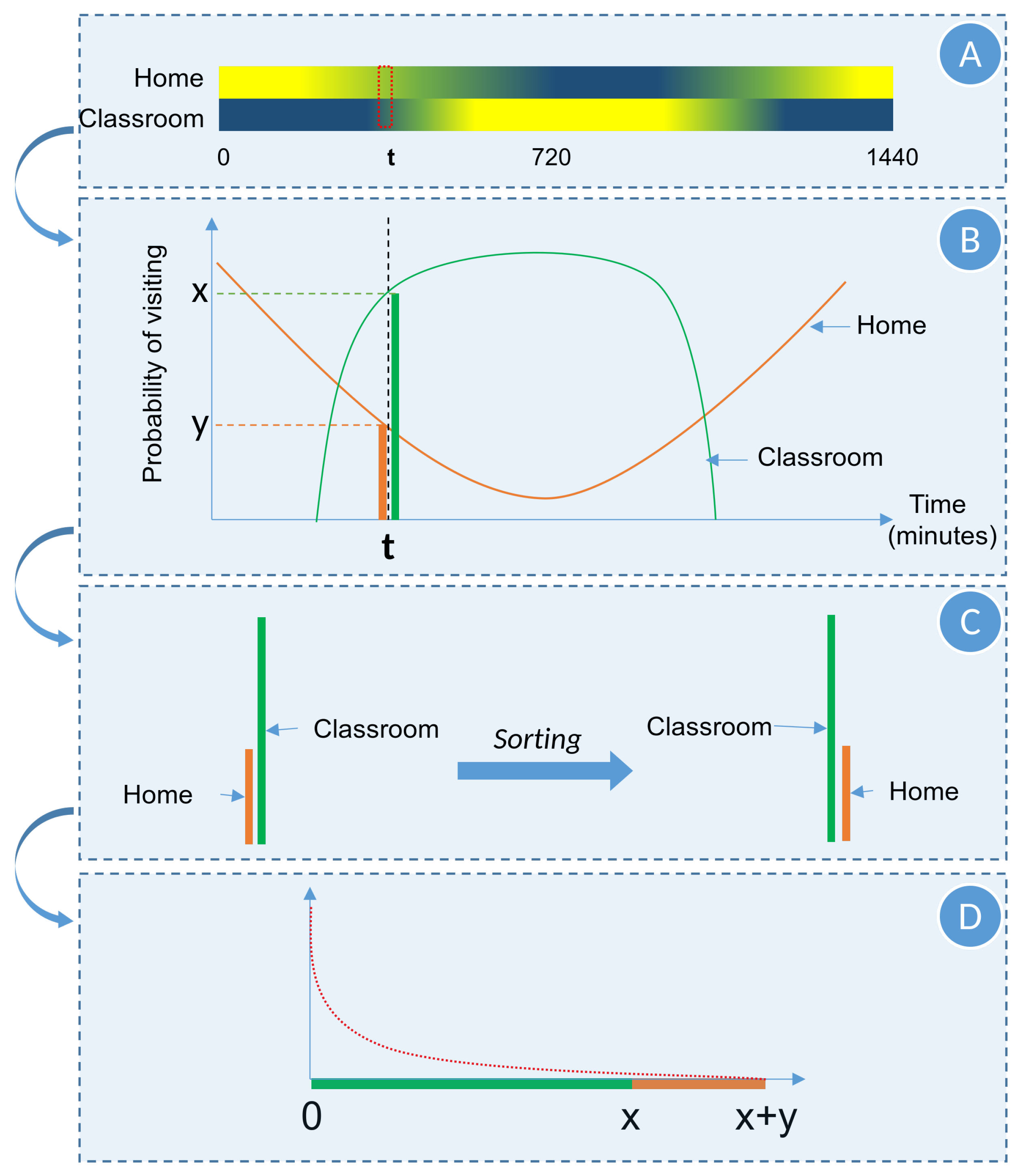
as illustrated in
Figure 4. Then, the location is selected giving higher priority to the places having high visit probability. In order to perform this selection the visit probabilities at time
t are sorted in descending order and a random number is selected from the exponential probability distribution illustrated in
Figure 4 (The motivation for selecting an exponential distribution with
rate parameter is to increase the chance of picking a location with large probability values). Finally, the location type is selected by projecting the random number onto the horizontal axis.
According to the example in
Figure 4, if the randomly generated number is between 0 and
x, we select the “Classroom” location type as the next location type of the daily routine. If it is between
x and
, the “Home” location type will be selected. The extracted visit-probability values are stacked along the x-axis as illustrated in
Figure 4.
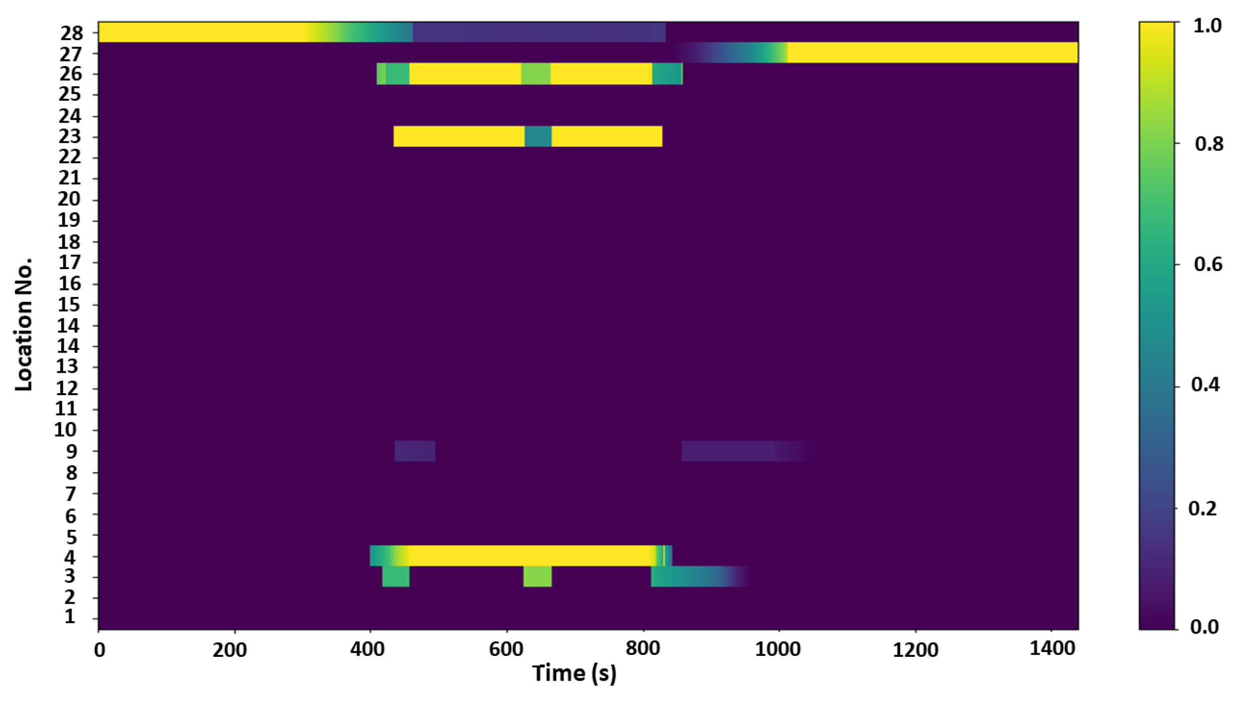
A visualization of the visit-probability matrix for the student class is illustrated in
Figure 5 where the time of the day (minutes) is given on the x-axis, and the y-axis represents different location types using location numbers (Location No).
The intensity of the color shown in the color bar on the right indicates the likelihood of visiting a particular location represented by a number between 0 and 1, where a higher value means that the agent is more likely to visit that location. In PDSIM, an agent has its own home, workplace, and weekend home location, and their visit-probability values are represented through the rows corresponding to Location No. 26, 24, and 25 respectively in
Figure 5. Therefore, when initializing the daily routine, if one of these unique locations were selected as the following location, PDSIM will choose the specific location assigned to the particular agent instead of the closest location of the selected location type. For the student example in
Figure 4, visit-probability values for these unique locations are illustrated in the first three rows.
The above-mentioned unique and fixed places for an agent further assures the generation of non-identical routines for agents. For example, consider two agents from classes X and Y (two agents are and ). Then the route for is not the same as ’s route because their home and working place is different. Thus, they will take different paths, and also they might go to different intermediate locations as well. When considering two agents from the same class X (two agents are and ). Let the home and working place of two agents be , and , from location classes H and W. Even though the location classes of the two agents are similar, the locations that they visit will be different. For example, the route of can be and the route of can be where r is a retail shop.
Location occupancy-probability matrix , gives the probability of a particular agent staying in a location. Each agent class (based on their occupation) has a unique matrix. The use of removes the Markov-ness (dependency on the previous location) of our daily routines. It removes the potential for unstable oscillations among locations through a subtle manoeuvre. In addition, the time spent at a location is easily understandable graphically.
Let us assume that “Classroom” was selected as the next location type, and a specific location of that type has been chosen to add to the daily routine. Now, it is necessary to decide how long an agent will stay in that particular location. This duration of staying varies with the type of agent (occupation) and the location where the agent will stay. Thus,
defines the probability of the agent staying in each location type for a given duration. The selection process of duration for “Classroom” is illustrated in
Figure 6, where a random period is selected according to the shown probability distribution. Thus, the chosen random duration for the agent who will go to “Classroom” should be a value most likely around 0, 40, or 80 minutes. This gives a more realistic duration for a student staying in a classroom where it can be assumed that a single subject will be taught for multiple 40-minute periods.
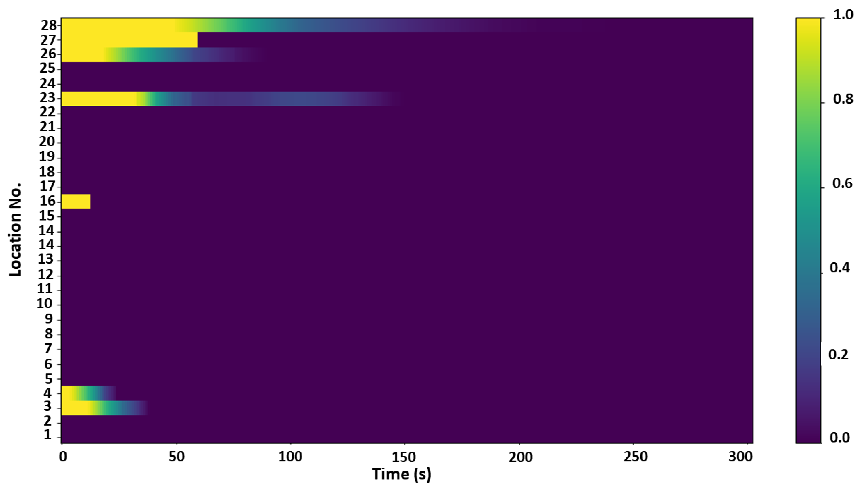
For the same student class, the overall occupancy-probability matrix
is given in
Figure 7 where the duration of staying in a location (in minutes) is provided in the x-axis, and the y-axis represents different location types as Location No. The intensity of the color given in the color bar on the right indicates the likelihood of staying in a particular location for a given period, where a higher value means that the agent is more likely and vice versa. The duration of staying in a location can be selected by randomly choosing a duration based on the probability density function of the
matrices’ corresponding row designated for that particular location. Both
and
mentioned above can be redefined for specific days. For example, on the weekend, people’s daily routine is very different from a weekday and more similar to a holiday. Therefore, there are multiple matrices for different types of days, and they are selected according to the day of the week.
3.5.2. Mobility Patterns
As mentioned in the previous section the movement can be categorized into two types: intra-location movement and inter-location movement. Intra-location movement pattern mainly depends on the location type. The movement of an agent can vary from being stationary to high mobility. The random movement can be controlled by increasing or decreasing the velocity randomly for horizontal and vertical directions.
When moving between locations an agent must initially move to the existing point of the current location. Then, the agent travels toward the next location. Unlike the stochastic movement explained earlier, as the agent has a target position that they should reach, the agent should move towards the entrance point of the next location in a predefined line between two locations.
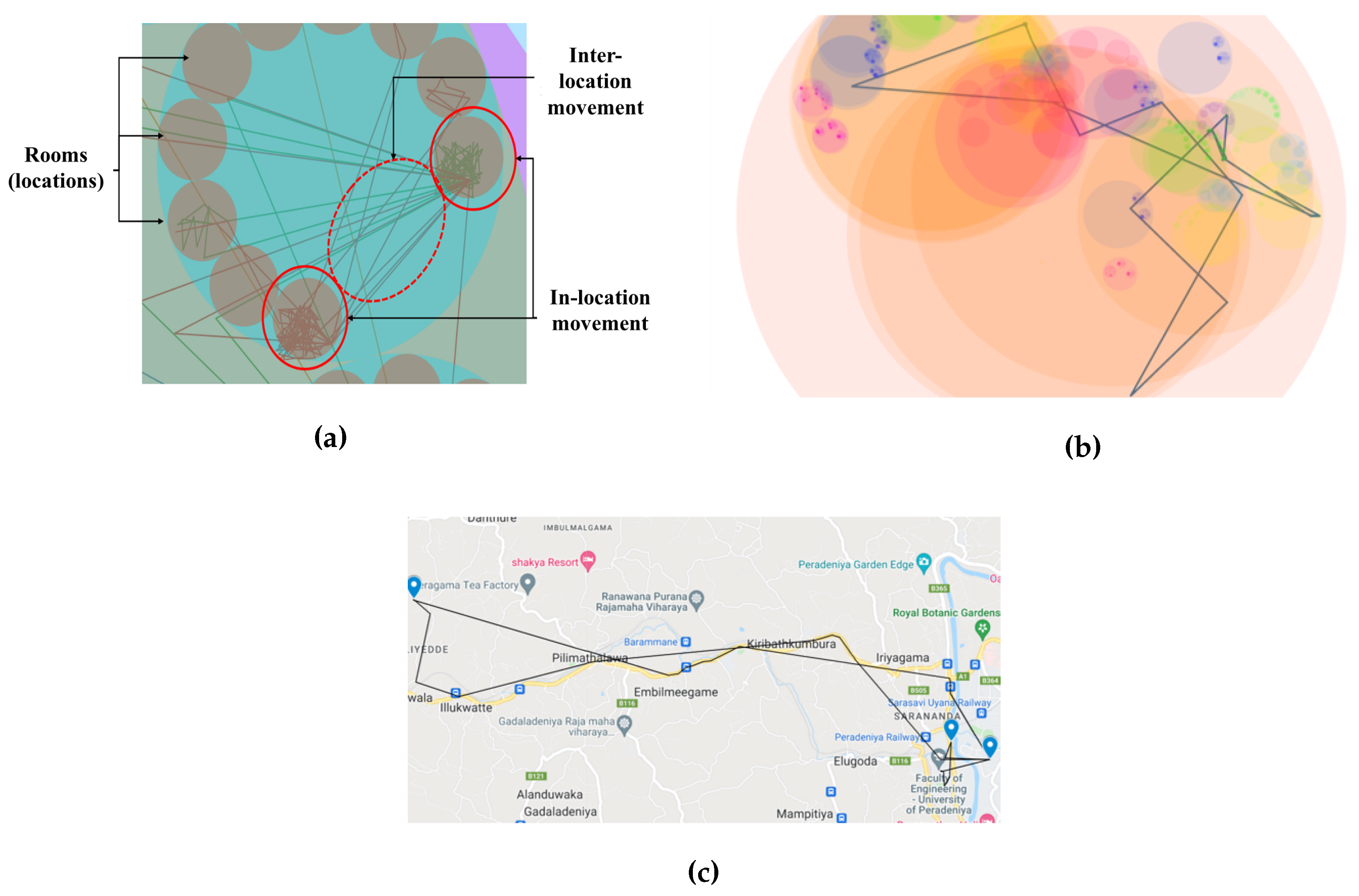
Figure 8a illustrates a part of the environment in a particular simulation. It shows the path taken by an agent inside a location (intra-location motion) and the path taken when moving in between two locations. The circular shapes represent different places in the environment (for example, a room, building, etc.).
Figure 8c shows an actual path taken by a person in the real world on a particular day. The path taken by an agent in the simulator, as illustrated in
Figure 8b is similar to the real-world path where one can see a stochastic motion when a person is occupied with a specific task inside a location and a discrete movement or a “jump” when people are moving between two locations.
Even though these two movement methods can model the basic movements of an agent, one should consider more factors associated with the mobility of an agent to simulate disease transmission properly. For example, the moving speed can vary from each movement system. Also, if the agent uses a vehicle for movement, they can be isolated from other agents using another vehicle. Therefore, different movement systems are introduced in PDSIM to tackle some of these problems.
3.5.3. Movement Systems
The movement characteristics of an agent when moving around a location is different from the movement when an agent is moving from one location to another. For example, when an agent is in a building, the agent can walk around slowly while interacting with other agents in the building. But when an agent moves between two cities, the agent may use a private vehicle and he/she will have very few interactions with agents they encounter. However, if the agent uses a public transportation method like a bus, the agent will interact with other passengers in the same vehicle. In the stated scenarios unique movements, interactions, and disease transmission dynamics vary from one to another.
In PDSIM at the beginning of the simulation, each agent is assigned to a particular movement system responsible for the agent’s movement. This is randomly selected from a set of movement methods assigned for a given occupation. The set of movement methods reflects the agent’s occupation and economic standing (e.g., the administrative agent is likely to use their private vehicle, whereas an average commercial worker might use public transport vehicle). The movements can vary from simple walking in a building or driving a car to a more complex movement system where one agent transports several other agents, similar to a bus driver. In every location change of an agent, they are assigned to a movement system and subjected to that system’s disease transmission dynamics.
The simulator consists of two central movement systems. Independent Movement Systems (IMS) operate independently of other movement systems. Independent movement methods such as walking or travelling using a personal vehicle fall into this category. If an agent who is using an IMS intends to move to another location or roam around, he/she can initiate the movement without waiting for transport.
If an agent is moved by a transporter then it is modeled under Dependent Movement Systems (DMS). In this, transporter agents are responsible for moving other agents around the environment. Some examples of these movement systems are buses and taxis. In these systems, travellers cannot move unless they enter a vehicle driven by a particular transporter agent. Transporter agents follow a specific daily routine where they move, passing different locations. When these transporter agents approach a specific location, if there are travellers who want to travel to a destination where the driver agent is also going, those travellers will latch onto the transporter agent. The maximum capacity that a transport agent can move at a time is assigned based on the mode of transport (vehicle). For example, a taxi driver can accommodate up to 3 passenger agents, and a bus driver can accommodate up to 60 passengers. Therefore, in contrast to the previously mentioned IMS, agents cannot immediately move when they want to travel to another location. They have to wait at a "stand/stop" until public transport is available, much like reality. When an agent reaches the destination location, the movement system will be changed to the settings used in the destination location. If a location is quarantined or isolated the agents won’t be able to leave the location until the containment is lifted off.
Each agent has a preferred movement mode. Therefore, all agents will not use the same movement system when travelling between locations. This preference will be overridden if the locations enforce a default movement system through an overriding level. In that case, the agents cannot use their favourite method, but they should compel with the regulations in the location. For example, movement systems implemented for walking, cars, and buses can have an overriding level of 1, 4, and, 9 respectively. This ensures that the car owners will use their vehicles even though travelling by bus is an option, but they cannot use the car in a walking area such as a park.
The proposed movement system ties well with the combined random and discrete motion style. This novel system is used to model the paths taken by agents realistically in collaboration with other features of PDSIM. Furthermore, this enables the assessment of vulnerabilities in the transport sector and helps to determine the effectiveness of social distancing practices in public transport.
3.6. Interventions
PDSIM provides additional features on top of the mobility and disease propagation models to include different dynamics of the society into the simulation. These additional features can be utilized in implementing policies to improve the resilience of the environment to diseases such as Covid-19.
3.6.1. Physical Distancing
The distance between two people directly impacts how the disease will spread. Different levels of social distancing practices are implemented in different locations. In the real world, some places such as supermarkets, hospitals, banks, etc. impose social distancing protocols inside the premises. The agent in PDSIM will maintain social distancing adhering to the protocol implemented by the locations, unless the agents’ personal opinion overrides it.
The physical distancing intervention can be used to identify the effectiveness of social distancing measures for different locations. Furthermore, this enables the user to implement different regulation measures to gauge their impact for a given location and, identify the general variation of the infection statistics.
3.6.2. Hygiene
The hygiene of an individual contributes to the disease spread on a major scale. However, the likelihood of imposed hygienic practices varies form person to person. During Covid-19, certain locations made basic hygienic practices such as using sanitiser, washing hands with soap, etc. and, they were mandatory to follow before entering a particular place. In the light, the PDSIM has introduced a property to reflect the hygiene of an agent. The value of this property will be lower if an agent follows good sanitary practices and vice versa. In some locations, the hygiene of the agents will be boosted in order to model the effect of implementing good hygiene practices.
3.6.3. Testing, Diagnosis, Quarantine and Isolation of Positives Agents
PDSIM tries to realistically perform the testing and diagnosis of infected agents. Testing is carried out randomly in the medical zones. If an agent is symptomatic, there is a higher chance of selecting the particular agent when randomly selecting the agents for testing. Moreover, a limit is assigned for the number of tests carried out in a single test centre on a given day. Once an agent is tested, there is a predefined lag prior to receiving the test results. Different testing methods such as PCR and the anti-gen test are designed with different testing accuracy to imitate the real-world scenario. Once an agent is tested positive for Covid-19, PDSIM sends either that patient to a Covid-19 treatment center or treated at their quarantined home.
3.6.4. Contact Tracing
When a susceptible agent is infected with Covid-19 by another infected agent, the information about the infected source is stored to trace the contact. Further, the place and time information is used to analyze the vulnerable locations and identify critical periods when the disease spread. This will be helpful in understanding the mechanics of disease propagation based on location and occupation.
3.6.5. Vaccines and Treatments
PDSIM allows the user to schedule vaccination events and define a limit of the age group that will be vaccinated at a particular event. Users can define vaccination events that store the dates of the vaccination and the limit of the age group that will be vaccinated. During an event, the unvaccinated agent will be randomly selected from the given age group and vaccinated. Vaccination will increase the immunity of the agents making them resistant to the disease and less likely to spread the disease. In PDSIM, the immunity achieved through vaccination will decay by 1% each day ([
40]). This is equivalent to a reduction of the immunity boost given by vaccine to half through a period of two months). A vaccinated person is eligible for a second dose if the immunity boost falls low. PDSIM provides the opportunity to analyze the effect of the vaccination. The user can compare different vaccination strategies and different vaccines to select the optimum strategy which decreases the spread and the casualties of the disease.
3.6.6. Simulating Different Types of Social Events (Super Spreader Events)
Throughout the world, it has been observed that most of the new waves of Covid-19 started from a gathering event held when the containment measures were relaxed by the governing bodies of the locality. These sudden outbreaks were reinforced with different variants that spread faster, more severely and, caused massive societal disruptions. PDSIM provides the ability to design this kind of large gathering as super spreader events specifying the time, duration, maximum capacity, and characteristics of the people who might enter the event.
Adding super spreader events makes it possible to assess the effect of organizing such large events in a pandemic situation and analyze the overall statistical trends, such as the generation of new waves because gathering events create opportunities that enable interactions between isolated groups of people who otherwise do not interact.
3.7. Data Input User Interface (UI)
PDSIM allows the user to update basic parameters of the simulation, such as the number of simulation days, infection radius, incubation period, demographic information, etc. through a UI.
Furthermore, the user is able to design the environment through the UI. Users can create a wide array of environments that would best reflect the societies they hope to simulate and use them to replicate similar locations and variants that make the overall location structure. Also, the users can update the characteristics of each population group, define custom immunity levels, tendency to follow guidelines, preferential modes of transport, the practice of good hygiene in certain groups, and, social distancing likelihood, which are critical to disease spread. The UI provides the flexibility to easily add any interventions to the simulation using events such as gathering events, variant breed events, containment events, and vaccination events.
If the and were initiated using real-world survey data to mimic the behaviour of people in a certain locality or an occupation, PDSIM can be used to forecast the disease propagation patterns. Then the results can be used to identify vulnerable locations and occupation classes to test the effectiveness of containment strategies. Further, the users can observe how the mindset of the population changes with the pandemic. The outcomes of these simulations will assist the authorities to get preparing for waves of such communicable diseases and take better decisions to prevent the spread of the disease.
3.8. Software Architecture
PDSIM simulation engine was developed using Python 3.7 with the support of additional libraries. Libraries NumPy (numpy.org) and Pandas (pandas.pydata.org) were used for data manipulation, storing, and loading. Additionally, to parallelize the computational processes and increase the speed of calculation, a multiprocessing library was used. The simulation parameter adjustment, initialization and execution, and results visualization are made using the front end developed using ReactJS. The source code for PDSIM is available in GitHub. PDSIM is fully open-source, and you can find more information at
ai4covid.lk/simulator, with complete documentation and a comprehensive set of tutorials. A simple web app for PDSIM has been developed based on React.js (for the frontend), Flask (for communicating between the frontend and the backend), and Gunicorn/ NGINX (for running the server).
4. Results and Discussion
In this section, the operation of PDSIM is validated through the results obtained through simulations. Furthermore, the operation and effectiveness of the disease-related dynamics are observed, and their applicability to mitigating disease spread amidst a pandemic is discussed. In addition, PDSIM is used to compare the disease spread within the population by initializing the simulations by spawning infected agents among different classes of agents, for 120 days.
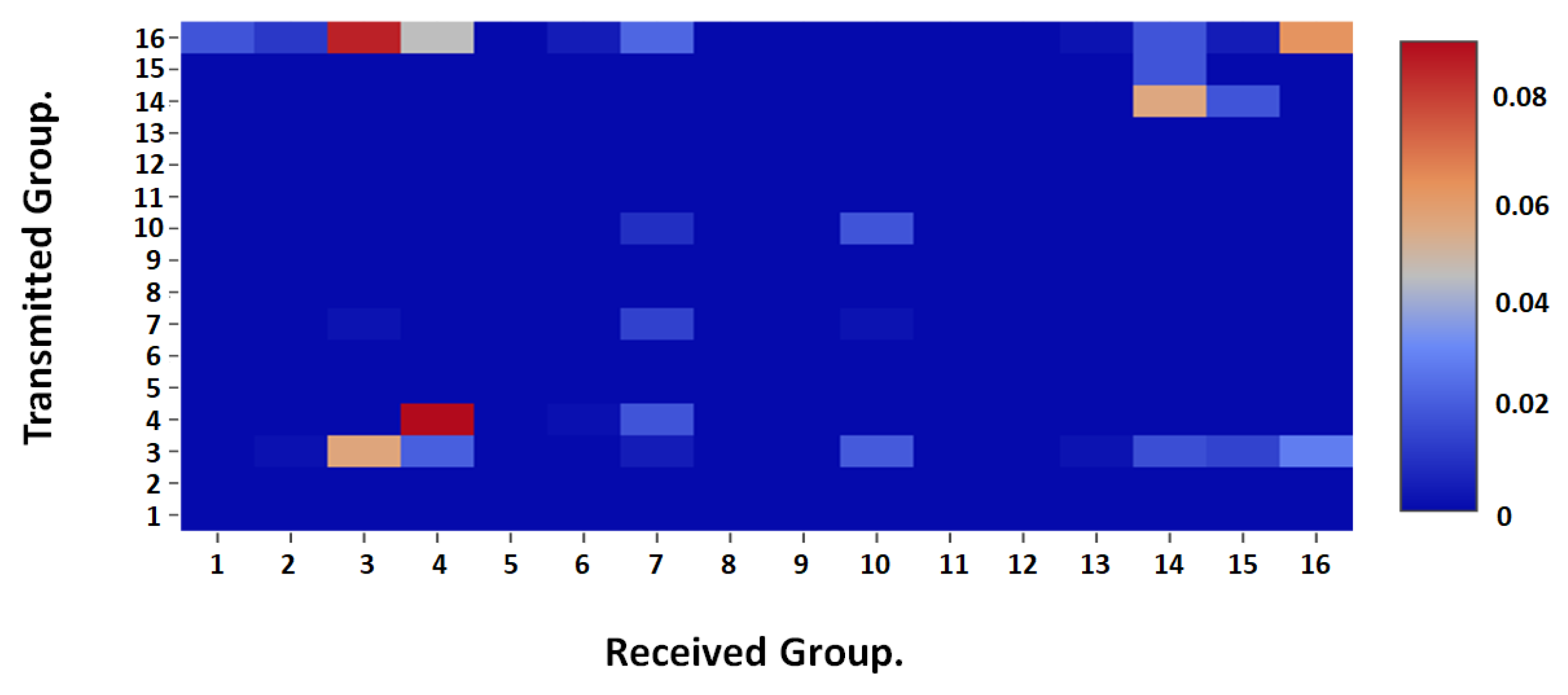
Initially, the disease transmission between different groups of agents was studied considering different occupations and age groups. For that purpose, infection events per infected person in each group was calculated with respect to other groups. For example, considering a grouping method by occupation, if there are 10 infected students on a given day, we estimate how many others in each occupation were infected by all 10 students and normalize them by the number of students. These values were calculated for each day and averaged to obtain the mean infections from one occupation to another within a day. Similarly, average infection events per day were calculated for all occupations, and it is illustrated in
Figure 9. This can be used to observe the transmission of the disease from one occupation class to another. This will aid healthcare workers and governments to identify potential groups who are susceptible to infection when an infected cluster is formed among a particular set of agents.
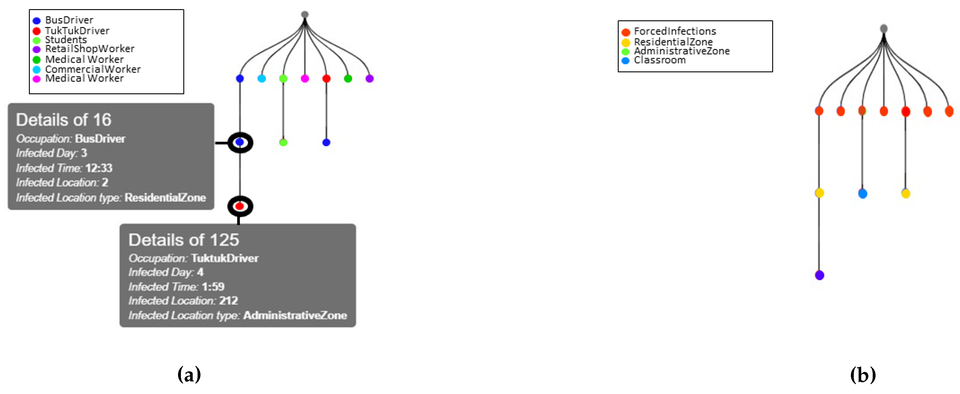
Furthermore, the granularity provided by the PDSIM enables intensive analysis to be done in terms of disease spread in a community. Through the infection propagation tree diagrams illustrated in
Figure 10, it allows the user to trace the infection transmission events.
Figure 10a, manifests the capability of PDSIM to pin point the disease transmission path among agents while
Figure 10b tracks where the infected contact happened. Once an environment is modeled and the demographic information is fed, the data provided by these propagation diagrams after simulation will help the governments to identify the next vulnerable groups and locations, so that pin point containment can be carried out rather than using city-wide lockdown strategies which affect the social and economical state of the community. Give on which sector (educational, transportation, commercial, etc.) the cluster initiated PDSIM can be used to identify how the infections are spread to the other sectors and locations by summarizing the infection tree diagrams.
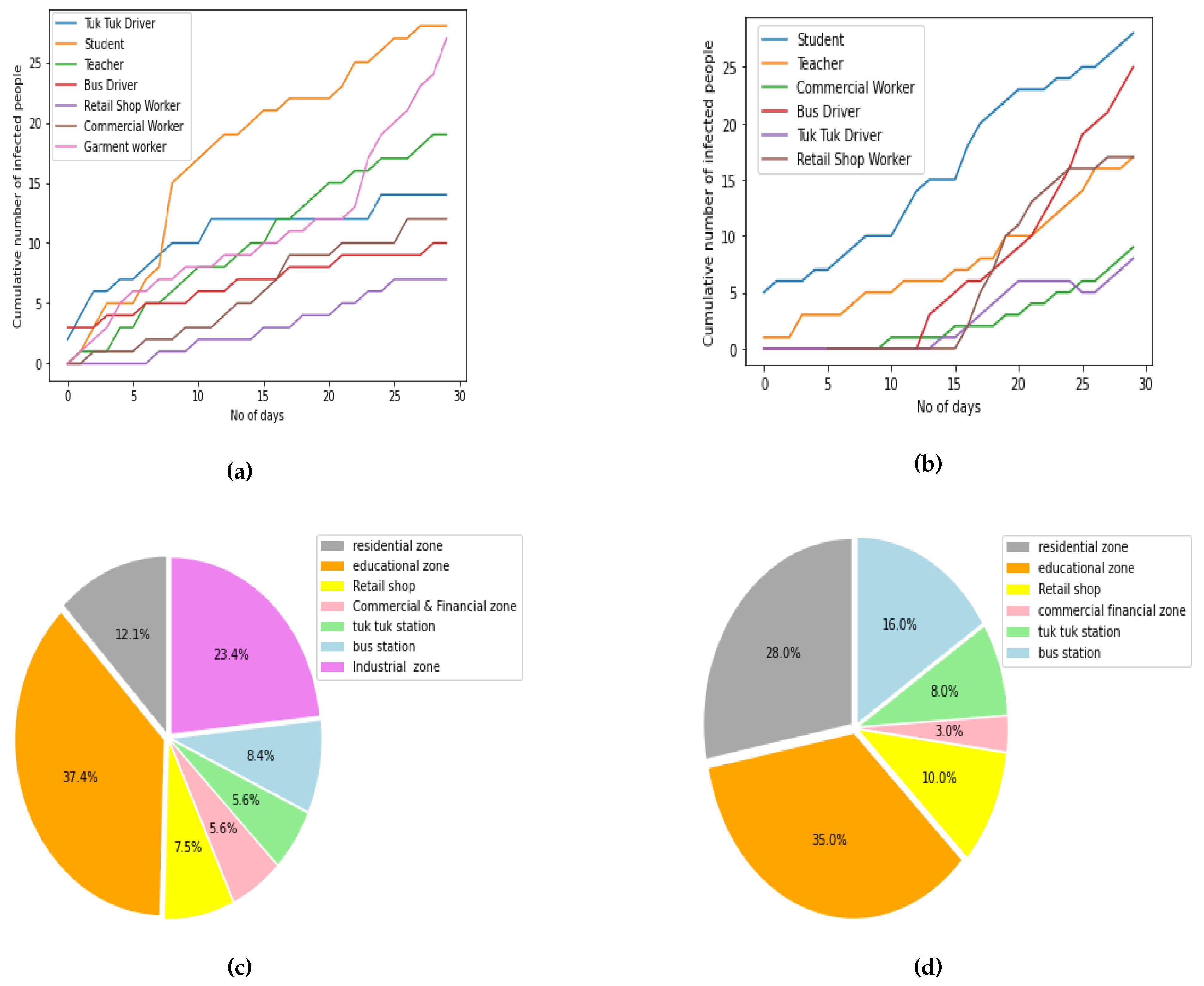
Figure 11a and,
Figure 11b summarize the cumulative number of infected cases from different occupations reported in the first 30 days when a simulation initiated by infecting agents from the transportation sector and education sector respectively. Observing the diagrams, it can be seen that the cluster initiated among the tuk-tuk drivers and bus drivers has rapidly spread to other occupation classes. Additionally, the pie charts encapsulate the infection summary with regard to locations. From this, the users can identify the most vulnerable locations once an outbreak occurs within a certain group of people. According to
Figure 11c, most of the infections happen within educational zones and industrial zones when a cluster is initiated in transportation sector. However, for an outbreak started in an educational sector, the second highest number of infectious contacts are reported inside residential zones as shown in
Figure 11d. The information conveyed from these types of analyses can be used by healthcare officials and governments to identify the locations within a city which are prone to spread the disease. By knowing these the officials can build up resilience within them by using proper policies. Once the susceptible locations are identified and isolated simple measures like improving hygienic practices and social distancing protocols can make an immense impact by reducing the disease spread. These will eventually make the community safe against the pandemic enabling uninterrupted operation of the essential industries and services making the community sustainable.
The ability to build complex environments through a simpler hierarchical tree structure allows easy customization of the environment through the environment builder to build different types of cities such as industrial cities, sparse districts, slums or suburbs, etc. As a result, an infection cluster’s propagation dynamics among different types of cities can be analyzed using PDSIM similar to
Figure 10 and
Figure 11. Through this, the way that the disease spread in diverse environments, once an infected cluster originated in a particular group of people can be predicted. For instance, a state government can identify the most vulnerable cities by taking factors such as demography and focus into account. Hence, decisions can be taken on a micro level to prevent outbreaks and mitigate the rapid spread of the diseases once an outbreak occurs in different cities making them resilient toward the pandemic.
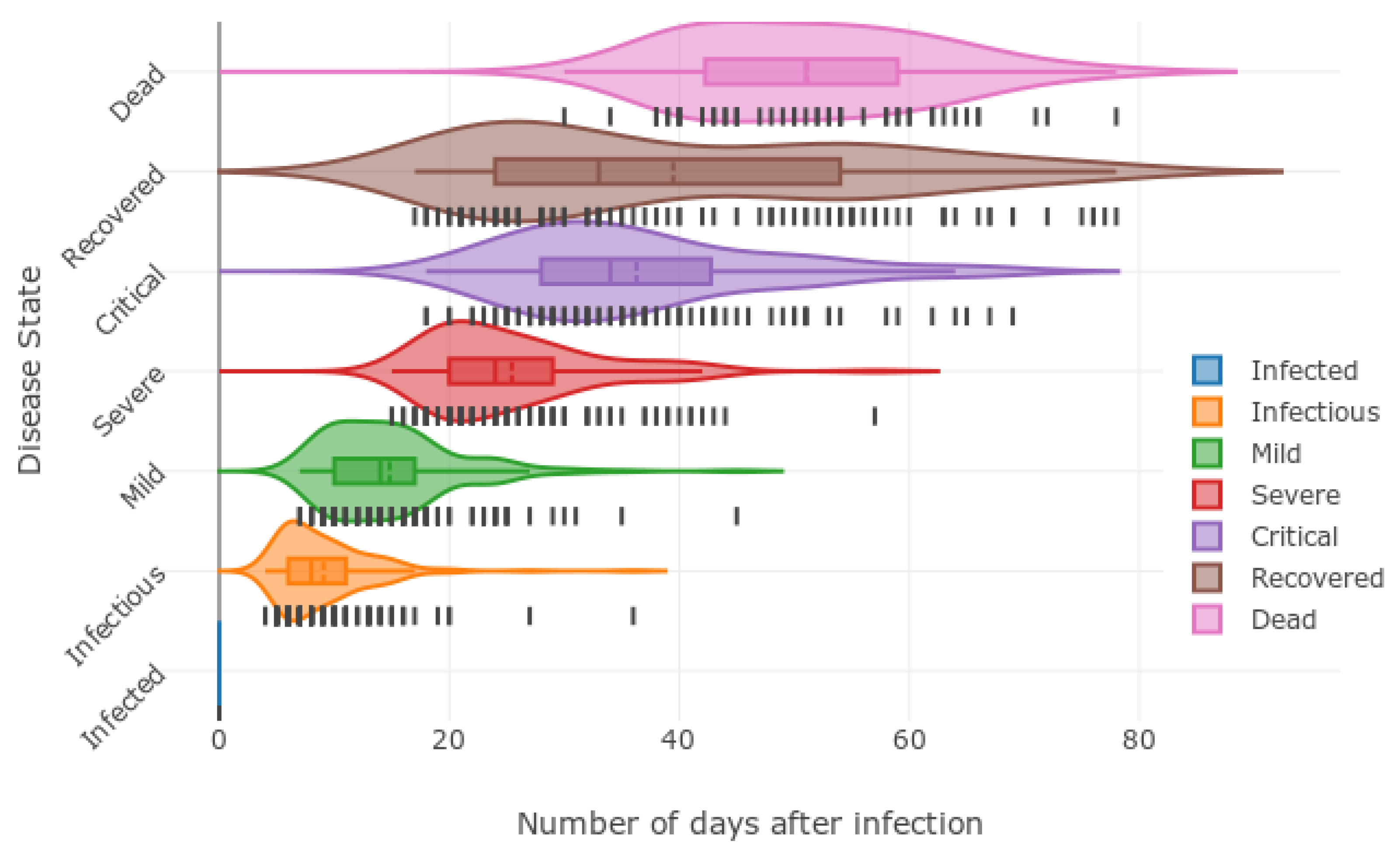
Next, the impact of the disease propagation modelling done according to
Figure 1 is observed through the violin diagram that is illustrated in
Figure 12. This provides an overview of the time taken by the disease to progress from one state to another. The data observed is illustrated in
Figure 12, where a kernel density estimation for each disease state is shown on top of a box and whisker diagram. This provides invaluable information such as the death ratio, incubation period, severity, and most importantly how long a wave would last. This highlights the importance of the violin plot in order to identify the essential characteristics of the dynamics of a given pandemic. The information on the time taken for disease state transmission can be considered as inherent to different variants. This allows the policymakers to foresee the threat and allocate the resources feasibly. For example, the health services can use the simulation results to predict the time window that will report a higher number of critical cases and strengthen their infrastructure.
After that, the effect of implementing different scenarios like gathering, vaccination, and containment events on the dynamics of the disease spread is explored.
Initially, a simulation was done to mimic the normal behaviour prior to the pandemic without any containment strategies or other protocols.
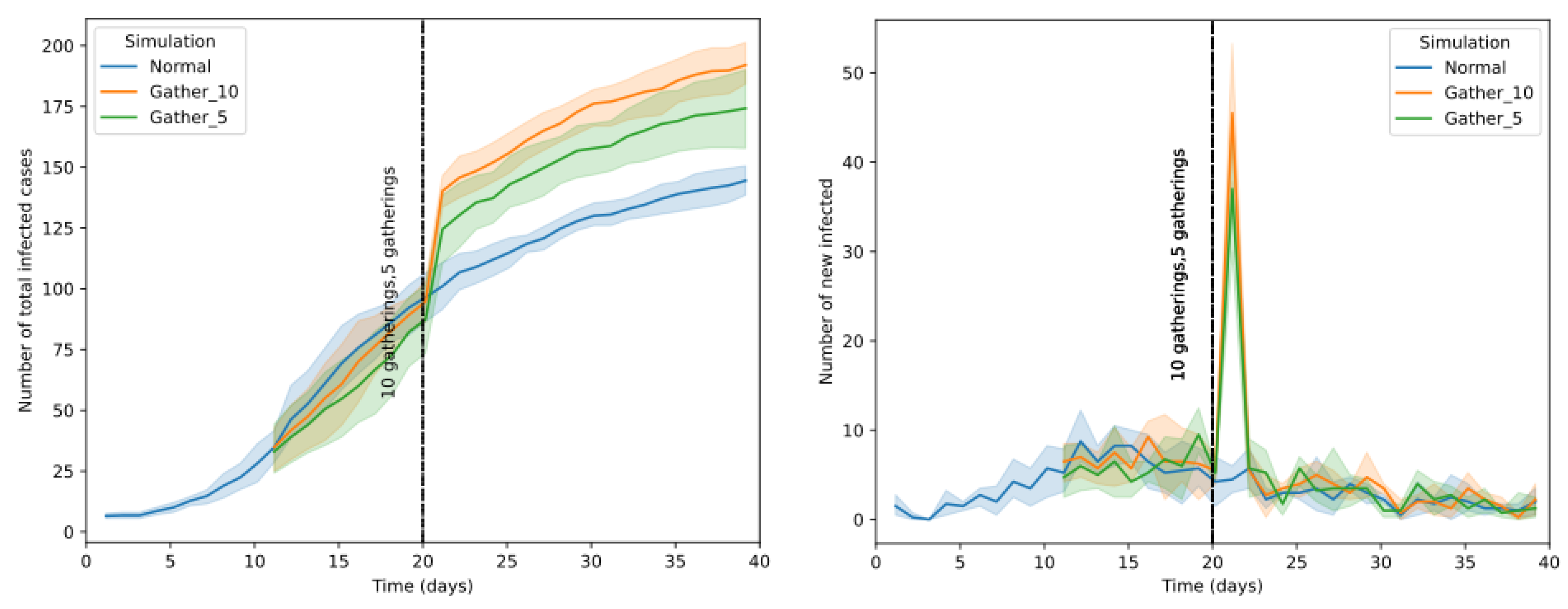
To investigate the response to super spreader events, several gathering events were scheduled on the 20th day of the simulation with a maximum capacity of 20 people per event. Then, the variation of the number of infections was observed by varying the number of events being 5 and 10 in consecutive simulations.
Figure 13, illustrates the simulated results which show the anticipated spike in the total number of infections and new infections after a gathering event is held. In addition, it can be seen that the number of new cases correlates with the number of gathering events held.
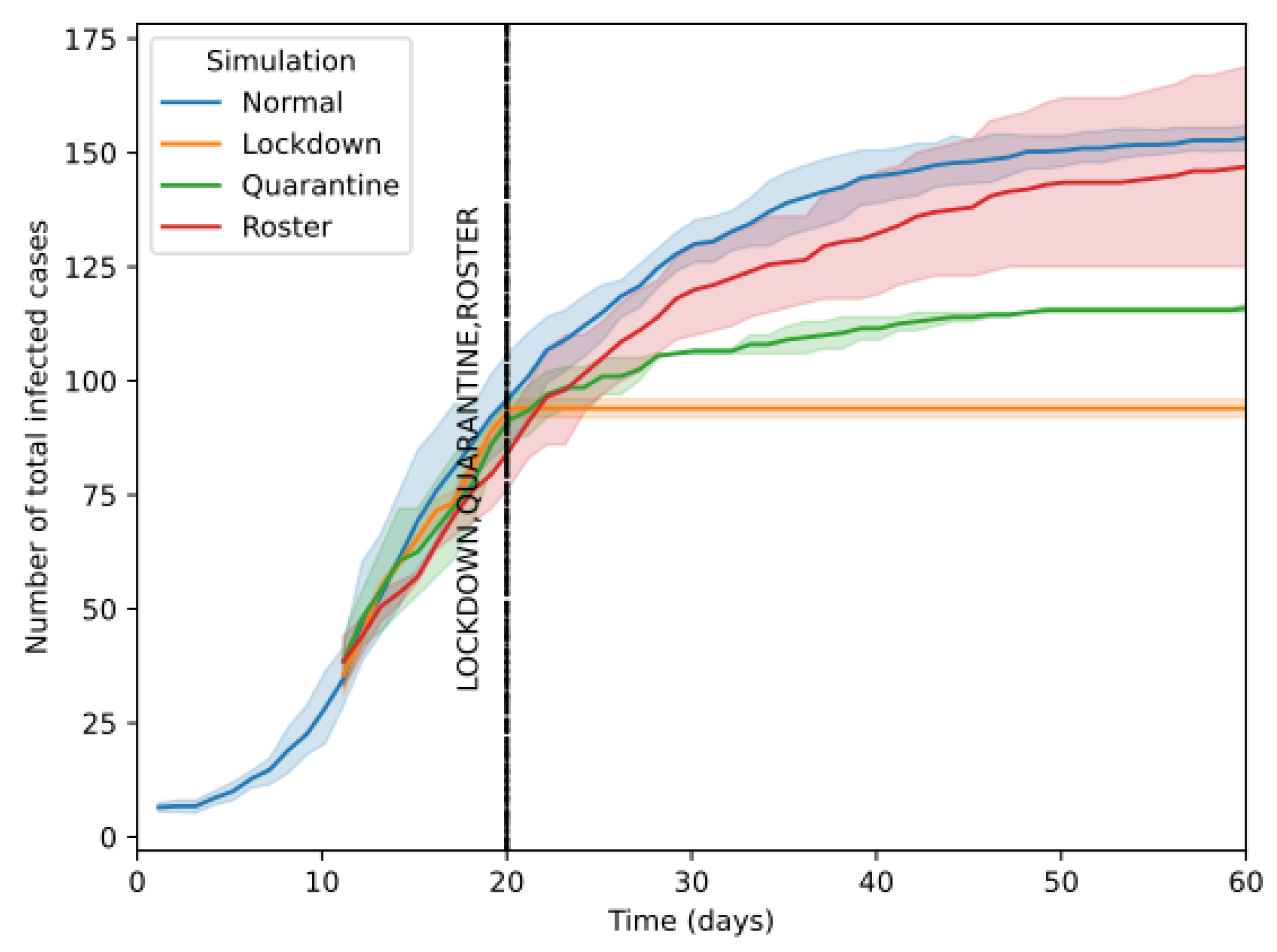
To analyze the effect of different containment strategies’ ability to curb disease spread, different containment policies were imposed on the 20th day of the simulation and the number of infected people for the following days was observed.
First, the simulation was done without interventions as the baseline observation. Next, a separate simulation with lockdown as the containment strategy is done. According to
Figure 14, it can be observed that when a lockdown containment is applied, it immediately reduces the number of new infections. However, the number of new infections does not go to zero because disease transmissions happen within people in a home where an infected person is living. It was observed that the lockdown containment procedure reduces the total infections by around 40% when compared with the simulation that does not implement any containment measures. Thereafter, a simulation in which a quarantine containment strategy starting from day 20 is carried out. During this people who tested positive for Covid-19 were quarantined in their respective households. According to
Figure 14, it can be seen that the reduction of new infections is minimal when compared with the lockdown containment strategy. When quarantine containment is implemented, those identified as infected agents will be home quarantined, which results in quarantining other members of the particular household. Therefore, there is a disease transmission within the house, but it is contained. Consequently, it can be observed that a small increment in the number of infected agents due to the disease spreading from unidentified infected agents as well as within-house infections in a quarantine containment strategy. The total number of infected agents was reduced by around 23% compared with the simulation with no containment measures. According to
Figure 14, it can be seen that the number of new infections with a roster-based containment strategy has an average total infection count below the normal case but with a high variance. This is because more infections occur at home, and those infected at home go outside and infect other people, increasing the number of new cases. The ability of PDSIM to capture this sensitive information allows it to be used to test the effectiveness of different containment strategies prior to imposing them.
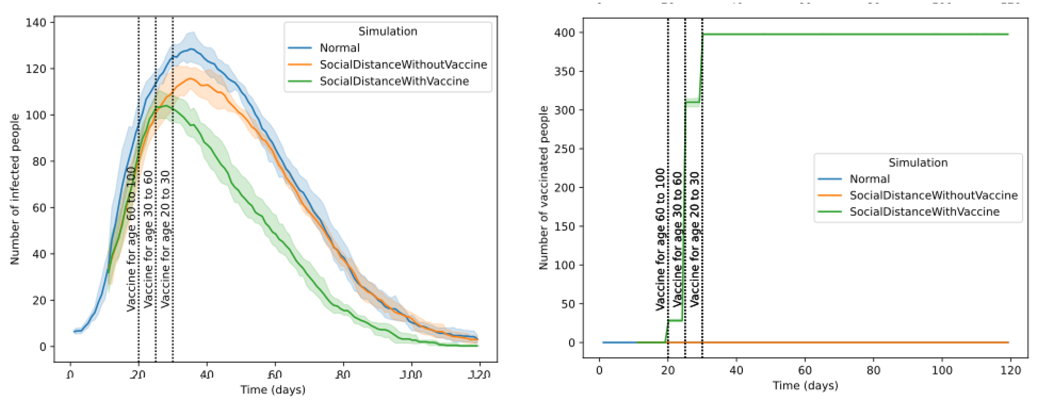
To mitigate the rapid spread of the pandemic it is vital to conduct the social distancing and vaccination strategies optimally.
Figure 15 shows the days and how vaccination is carried out for the population. The dashed line indicates the initiation of vaccination for a particular age group. The vaccination program will be conducted every day after initiation. The first dose of vaccination is given to all agents. The second dose of the vaccination is provided after a certain number of days when the immunity boost of the first dose is below a threshold value. The vaccine’s efficacy can be adjusted as a hyper-parameter to vary the number of new infections further.
Figure 15 compares the number of infected people under vaccination and without vaccination scenarios. The ability to compare the effect of vaccination depending on the dates, order of vaccination, type of vaccination and social distancing protocols can be used to make the vaccination program more effective.
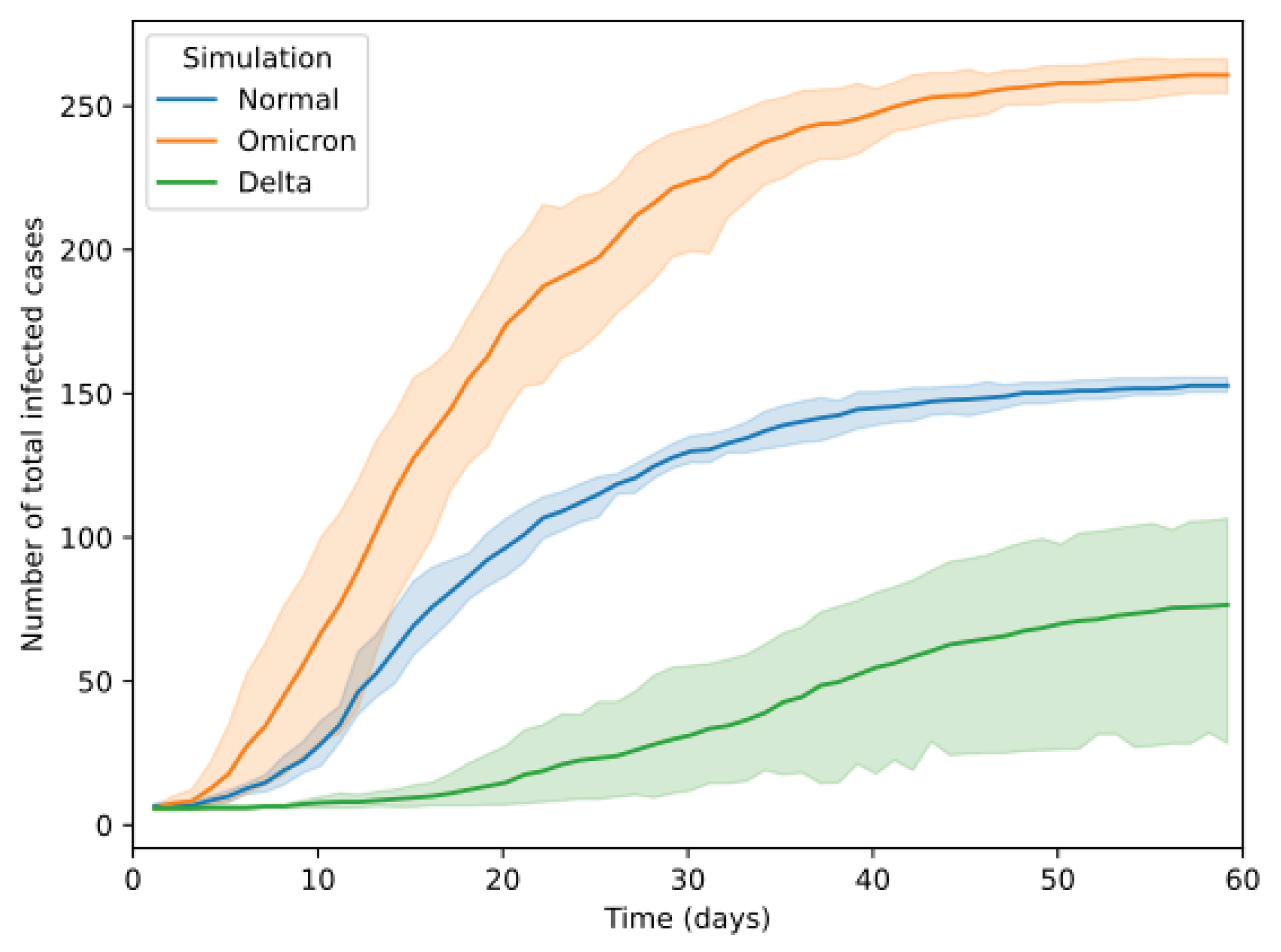
One of the significant turning points in the Covid-19 pandemic is the introduction of different variants of the disease by mutation. This spreads more severe variants like the "Delta variant" or a more transmittable variant like the "Omicron variant". To realize the behaviour of the variants modeled through PDSIM, two tests were conducted by introducing a more transmittable variant and a more severe variant to the population independently. Then, the total number of cases using the simulation is observed.
According to the illustration in
Figure 16, the number of infected patients for the severe variant did not increase as rapidly as the more transmittable variant. But the number of people in the critical state increased in the severe variant, and consequently, the number of deaths reported increased after a few days.
5. Implementation Strategies and Conclusions
The Covid-19 pandemic has disrupted the social and economic well-being of many countries across the world. In the aftermath of consecutive waves, some countries face dire consequences as the disease management strategies and policy implications were not effectively used to contain the disease. This study proposes an ABM PDSIM, which is capable of modeling complex environments and simulating realistic human behaviour in different population groups, to analyze the effect of different interventions on a pandemic.
The cities, states and countries in different parts of the world exhibit diversity in terms of infrastructure and demography. Understanding this diversity and inherent features of the population is imperative as the strategies to control the pandemic will vary accordingly. For example, containment measures needed to be taken in a large industrial district will differ from the measures needed in a suburban residential district. PDSIM grant the opportunity to design cities with different demographics and compare the robustness or the versatility of the cities in terms of being sustainable amidst a pandemic to make them more resilient, inclusive and sustainable.
PDSIM provides the ability to model complex environments using basic building blocks. The user can build an environment similar to the environment of interest and add demographic details based on the actual population statistics. Once the behaviour model is tuned according to the basic behavioural patterns of the population, the simulation can be carried out to mimic the real-world scenario of the region of interest. The ability to spawn infected agents amongst different categories of people (students, government workers, etc) allow the user to simulate the disease propagation and its effect on the population by varying the initial cluster of infected agents. Furthermore, the potential to see how occupations are linked through interactions allows us to identify the susceptible groups for disease transmission. In addition, the ability to extract and analyse the signatures of different pandemics and variants (violin plot) enables more robust resource allocation to be done in order to make healthcare services resilient and inclusive. From the outcomes, PDSIM provides the opportunity to identify vulnerabilities and the groups of people and locations which are more susceptible to the pandemic. Furthermore, it grants the opportunity to determine the sectors which are more susceptible (transport, education, manufacture, etc) to the disease.
As a result, policymakers can impose strategies effectively to mitigate the spread and casualties of the disease. Simulated results, will assist to build resilience among vulnerable groups of people and locations. The analysis on disease propagation allows to do precise containment allowing the community to operate normally ensuring social and economic sustainability. In addition, the competency to simulate the effectiveness of vaccination and other containment measures will provide insight into the outcomes of this decision, prior to them being implemented in the real world. The capability to simulate different variants and diseases allows the policymakers to understand the current threats and extrapolate the pandemic’s characteristics for future threats and take necessary actions to control the disease spread, while minimizing its impact on society, eventually making it and the environment inclusive, safe, resilient and sustainable.
References
- Benita, F. Human mobility behavior in COVID-19: A systematic literature review and bibliometric analysis. Sustain. Cities Soc. 2021, 70, 102916. [CrossRef]
- Ma, L.; Huang, Y.; Liu, T. Unequal impact of the COVID-19 pandemic on mental health: Role of the neighborhood environment. Sustain. Cities Soc. 2022, 87, 104162. [CrossRef]
- Fore, H.H.; Dongyu, Q.; Beasley, D.M.; Ghebreyesus, T.A. Child malnutrition and COVID-19: The time to act is now. Lancet 2020, 396, 517–518. [CrossRef]
- Ruiu, M.L. Mismanagement of Covid-19: Lessons learned from Italy. J. Risk Res. 2020, 23, 1007–1020. [CrossRef]
- Giacopelli, G.; others. A Full-Scale Agent-Based Model to Hypothetically Explore the Impact of Lockdown, Social Distancing, and Vaccination During the COVID-19 Pandemic in Lombardy, Italy: Model Development. JMIRx Med 2021, 2, e24630. [CrossRef]
- Kilani, M.; Diop, O.; Diop, N. Using Transport Activity-Based Model to Simulate the Pandemic. Sustainability 2023, 15, doi:10.3390/su15032257. [CrossRef]
- Kerr Cliff, S.R. Covasim: An agent-based model of COVID-19 dynamics and interventions. PLOS Computational Biology. [CrossRef]
- Gabler, J.; Raabe, T.; Röhrl, K. People Meet People: A Microlevel Approach to Predicting the Effect of Policies on the Spread of COVID-19 2020.
- Trivedi, A.; Sreenivas, N.K.; Rao, S. Modeling the Spread and Control of COVID-19. Systems 2021, 9, 53. [CrossRef]
- Wei, X.; Wang, L.; Jia, Q.; Xiao, J.; Zhu, G. Assessing different interventions against Avian Influenza A (H7N9) infection by an epidemiological model. ONE Health 2021, 13, 100312. [CrossRef]
- Salje, H.; Tran Kiem, C.; Lefrancq, N.; Courtejoie, N.; Bosetti, P.; Paireau, J.; Andronico, A.; Hozé, N.; Richet, J.; Dubost, C.L.; Le Strat, Y.; Lessler, J.; Levy-Bruhl, D.; Fontanet, A.; Opatowski, L.; Boelle, P.Y.; Cauchemez, S. Estimating the burden of SARS-CoV-2 in France. Science 2020, 369, 208–211. [CrossRef]
- Atkeson, A.; others. On using SIR models to model disease scenarios for COVID-19. Q. Rev. 2020, 41, 1–35. [CrossRef]
- Kermack, W.O.; McKendrick, A.G.; Walker, G.T. A contribution to the mathematical theory of epidemics. Proc. R. Soc. London. Ser. A, Contain. Pap. A Math. Phys. Character 1927, 115, 700–721, [https://royalsocietypublishing.org/doi/pdf/10.1098/rspa.1927.0118]. [CrossRef]
- Tsori, Y.; Granek, R. Epidemiological model for the inhomogeneous spatial spreading of COVID-19 and other diseases. PLoS ONE 2021, 16, e0246056. [CrossRef]
- Berger, D.; Herkenhoff, K.; Huang, C.; Mongey, S. Testing and reopening in an SEIR model. Review of Economic Dynamics 2020. [CrossRef]
- Wu, Z.; Wang, Y.; Gao, J.; Song, J.; Zhang, Y. A Multistage Time-Delay Control Model for COVID-19 Transmission. Sustainability 2022, 14, doi:10.3390/su142114657. [CrossRef]
- Keeling, M.J.; Hollingsworth, T.D.; Read, J.M. Efficacy of contact tracing for the containment of the 2019 novel coronavirus (COVID-19). J. Epidemiol. Community Health 2020, 74, 861–866[https://jech.bmj.com/content/74/10/861.full.pdf]. [CrossRef]
- Gaspar, R.M.; Prasetyo, Y.T.; Mariñas, K.A.; Persada, S.F.; Nadlifatin, R. Exploring Consumers’ Intention to Use Bikes and E-Scooters during the COVID-19 Pandemic in the Philippines: An Extended Theory of Planned Behavior Approach with a Consideration of Pro-Environmental Identity. Sustainability 2023, 15. [CrossRef]
- Bedoya-Maya, F.; Calatayud, A.; Giraldez, F.; Sánchez González, S. Urban mobility patterns and the spatial distribution of infections in Santiago de Chile. Transp Res Part A Policy Pr. 2022, 163, 43–54. [CrossRef]
- Ferguson, N.; Laydon, D.; Nedjati Gilani, G.; Imai, N.; Ainslie, K.; Baguelin, M.; Bhatia, S.; Boonyasiri, A.; Cucunuba Perez, Z.; Cuomo-Dannenburg, G.; others. Report 9: Impact of non-pharmaceutical interventions (NPIs) to reduce COVID19 mortality and healthcare demand 2020. [CrossRef]
- Rockett, R.J.; Arnott, A.; Lam, C.; Sadsad, R.; Timms, V.; Gray, K.A.; Eden, J.S.; Chang, S.; Gall, M.; Draper, J.; others. Revealing COVID-19 transmission in Australia by SARS-CoV-2 genome sequencing and agent-based modeling. Nat. Med. 2020, 26, 1398–1404. [CrossRef]
- Aleta, A.; Martin-Corral, D.; y Piontti, A.P.; Ajelli, M.; Litvinova, M.; Chinazzi, M.; Dean, N.E.; Halloran, M.E.; Longini Jr, I.M.; Merler, S.; others. Modelling the impact of testing, contact tracing and household quarantine on second waves of COVID-19. Nat. Hum. Behav. 2020, 4, 964–971. [CrossRef]
- Kretzschmar, M.E.; Rozhnova, G.; Bootsma, M.C.; van Boven, M.; van de Wijgert, J.H.; Bonten, M.J. Impact of delays on effectiveness of contact tracing strategies for COVID-19: A modelling study. Lancet Public Health 2020, 5, e452–e459. [CrossRef]
- Lau, M.S.; Grenfell, B.; Thomas, M.; Bryan, M.; Nelson, K.; Lopman, B. Characterizing superspreading events and age-specific infectiousness of SARS-CoV-2 transmission in Georgia, USA. Proc. Natl. Acad. Sci. 2020, 117, 22430–22435. [CrossRef]
- Butt, A.; Ahmad, W.; Rafiq, M.; Baleanu, D. Numerical analysis of Atangana-Baleanu fractional model to understand the propagation of a novel corona virus pandemic. Alex. Eng. J. 2022, 61, 7007–7027. [CrossRef]
- Kaxiras, E.; Neofotistos, G. Multiple epidemic wave model of the COVID-19 pandemic: Modeling study. J. Med Internet Res. 2020, 22, e20912. [CrossRef]
- Haddad, H.; Bouyahia, Z.; Horchani, L. On the Sustainability of Shared Mobility Since COVID-19: From Socially Structured to Social Bubble Vanpooling. Sustainability 2022, 14, doi:10.3390/su142315764. [CrossRef]
- Wang, Z.; Yang, J.; Zhang, Q.; Wang, L. Risk-Aware Travel Path Planning Algorithm Based on Reinforcement Learning during COVID-19. Sustainability 2022, 14, doi:10.3390/su142013364. [CrossRef]
- Kuzdeuov, A.; Baimukashev, D.; Karabay, A.; Ibragimov, B.; Mirzakhmetov, A.; Nurpeiissov, M.; Lewis, M.; Varol, H.A. A network-based stochastic epidemic simulator: Controlling COVID-19 with region-specific policies. IEEE J. Biomed. Health Informatics 2020, 24, 2743–2754. [CrossRef]
- Kompella, V.; Capobianco, R.; Jong, S.; Browne, J.; Fox, S.; Meyers, L.; Wurman, P.; Stone, P. Reinforcement learning for optimization of COVID-19 mitigation policies. arXiv preprint arXiv:2010.10560 2020. [CrossRef]
- Ng, K.Y.; Gui, M.M. COVID-19: Development of a robust mathematical model and simulation package with consideration for ageing population and time delay for control action and resusceptibility. Phys. D: Nonlinear Phenom. 2020, 411, 132599. [CrossRef]
- Lemaitre, J.C.; Grantz, K.H.; Kaminsky, J.; Meredith, H.R.; Truelove, S.A.; Lauer, S.A.; Keegan, L.T.; Shah, S.; Wills, J.; Kaminsky, K.; others. A scenario modeling pipeline for COVID-19 emergency planning. Sci. Rep. 2021, 11, 1–13. [CrossRef]
- Gorji, H.; Arnoldini, M.; Jenny, D.; Hardt, W.D.; Jenny, P. Dynamic modelling to identify mitigation strategies for the COVID-19 pandemic. Swiss Med Wkly. 2021, 151, w20487. [CrossRef]
- Chao, S.P. Simplified model on the timing of easing the lockdown. Chin. J. Phys. 2021, 70, 170–181. [CrossRef]
- Hinch, R.; Probert, W.J.; Nurtay, A.; Kendall, M.; Wymant, C.; Hall, M.; Lythgoe, K.; Bulas Cruz, A.; Zhao, L.; Stewart, A.; others. OpenABM-Covid19—An agent-based model for non-pharmaceutical interventions against COVID-19 including contact tracing. PLoS Comput. Biol. 2021, 17, e1009146. [CrossRef]
- Kuzdeuov, A.; Karabay, A.; Baimukashev, D.; Ibragimov, B.; Varol, H.A. A Particle-Based COVID-19 Simulator with Contact Tracing and Testing. IEEE Open J. Eng. Med. Biol. 2021, 2, 111–117. [CrossRef]
- Barak, O.; Gavish, N.; Hari, L.P.; Shohat, T. Simulator of interventions for COVID-19, 2020.
- Mellacher, P. COVID-town: An integrated economic-epidemiological agent-based model. arXiv preprint arXiv:2011.06289 2020. [CrossRef]
- Shamil, M.S.; Farheen, F.; Ibtehaz, N.; Khan, I.M.; Rahman, M.S. An agent-based modeling of COVID-19: Validation, analysis, and recommendations. Cognitive Computation 2021, pp. 1–12. [CrossRef]
- Ledford, H.; Cyranoski, D.; Van Noorden, R.; others. The UK has approved a COVID vaccine—here’s what scientists now want to know. Nature 2020, 588, 205–206. [CrossRef]
Figure 1.
A graphical representation of the Disease State Propagation Diagram. Lognormal (logN) values displayed on the edges represents the time taken for the disease state transition.
Figure 1.
A graphical representation of the Disease State Propagation Diagram. Lognormal (logN) values displayed on the edges represents the time taken for the disease state transition.
Figure 2.
Hierarchical connection of locations to model the environment.
Figure 2.
Hierarchical connection of locations to model the environment.
Figure 3.
Illustration of the difference between completely random movement and a combined random and discrete movement.
Figure 3.
Illustration of the difference between completely random movement and a combined random and discrete movement.
Figure 4.
Selection of the next location to visit using the visit-probability matrix.
Figure 4.
Selection of the next location to visit using the visit-probability matrix.
Figure 5.
Location visit-probability matrix for a student
Figure 5.
Location visit-probability matrix for a student
Figure 6.
Selection of the duration of staying in a location using the occupancy-probability matrix.
Figure 6.
Selection of the duration of staying in a location using the occupancy-probability matrix.
Figure 7.
Probability of staying in a given location by a student in PDSIM.
Figure 7.
Probability of staying in a given location by a student in PDSIM.
Figure 8.
(a) Part of the map view of the simulated environment and examples of agents moving in the environment. Lines represent the paths taken by different agents. (b) A path history of an agent on a particular day in PDSIM. Lines represent the paths taken by the agent.(c) A path history of a real person on a particular day where GPS locations were recorded using Google. Lines represent the paths taken by the person.
Figure 9.
Infection events are stratified by the occupation of source and recipient.(Occupations are labeled as Numbers as in
Table 3.
Figure 9.
Infection events are stratified by the occupation of source and recipient.(Occupations are labeled as Numbers as in
Table 3.
Figure 10.
(a) Part of a disease propagation tree diagram for the analysis of infection spread. (b) Part of a location tree diagram. Lines represent the paths taken by the agent.
Figure 10.
(a) Part of a disease propagation tree diagram for the analysis of infection spread. (b) Part of a location tree diagram. Lines represent the paths taken by the agent.
Figure 11.
(a) Infection count variation for a cluster started within transportation sector. (b) Infection count variation for a cluster started within education sector. (c) Percentage of infections that occurred at a location from the total number of infections for a cluster started in transportation sector (d) Percentage of infections that occurred at a location from the total number of infections for a cluster started in education sector
Figure 12.
Violin plot of the time took to progress the disease from one state to another after infection.
Figure 12.
Violin plot of the time took to progress the disease from one state to another after infection.
Figure 13.
Effect of holding gathering events on day 20 of the simulation.
Figure 13.
Effect of holding gathering events on day 20 of the simulation.
Figure 14.
Effect of implementing different containment strategies where all other parameters are kept constant.
Figure 14.
Effect of implementing different containment strategies where all other parameters are kept constant.
Figure 15.
Effect of social distancing and vaccinating protocols.
Figure 15.
Effect of social distancing and vaccinating protocols.
Figure 16.
The variation in total number of cases and number of deaths when different variants of the disease were introduced independently.
Figure 16.
The variation in total number of cases and number of deaths when different variants of the disease were introduced independently.
Table 1.
Comparison of disease simulators found in the literature with ours.
Table 1.
Comparison of disease simulators found in the literature with ours.
| Simulation method |
Simulator |
Features |
| Disease Progression |
Realistic human motion |
Hygiene simulation |
Public transport system |
Recreational activity |
Testing protocol |
Vaccination strategy |
Containment strategy |
Contact tracing |
Friendly User Interface |
Detailed daily routines |
Economical impact |
Super spreader event simulation |
| Compartment models |
A Network-Based Stochastic Epidemic Simulator [29] |
√ |
|
√ |
|
|
|
|
√ |
|
√ |
|
|
|
| PandemicSimulator [30] |
√ |
|
√ |
|
|
√ |
|
√ |
√ |
|
|
|
|
| Kermack–McKendrick model [31] |
√ |
|
|
|
|
√ |
|
|
|
√ |
|
|
|
| A scenario modeling pipeline for COVID-19 emergency planning [32] |
√ |
|
√ |
|
|
|
|
|
|
|
|
|
|
| Dynamic modelling to identify mitigation strategies for the COVID-19 pandemic [33] |
√ |
|
|
|
|
√ |
|
√ |
√ |
|
|
|
|
| Simplified model on the timing of easing the lockdown [34] |
√ |
|
|
|
|
|
|
√ |
|
|
|
√ |
|
| Agent based models |
Covasim [7] |
√ |
|
√ |
|
|
√ |
√ |
√ |
√ |
√ |
|
|
|
| OpenABM-Covid19 [35] |
√ |
|
|
|
|
√ |
|
√ |
√ |
|
|
|
|
| A Particle-Based COVID-19 Simulator [36] |
√ |
|
|
|
|
√ |
|
|
√ |
|
|
|
|
| Simulator of interventions for COVID-19 [37] |
√ |
|
√ |
|
|
√ |
|
√ |
√ |
|
|
|
|
| People Meet People [8] |
√ |
|
|
|
√ |
√ |
|
√ |
√ |
|
|
|
|
| COVID-Town [38] |
√ |
|
√ |
|
√ |
√ |
√ |
√ |
√ |
|
|
√ |
|
| An Agent-Based Modeling of COVID-19 [39] |
√ |
|
|
|
|
|
|
√ |
√ |
|
|
|
|
| Social Bubble Vanpooling (SBV) [27] |
√ |
|
|
√ |
|
√ |
|
√ |
√ |
|
|
|
|
| A road network impedance matrix based on SUMO Simulation [28] |
√ |
|
|
|
|
|
|
|
|
|
|
|
|
| PDSIM(Ours) |
√ |
√ |
√ |
√ |
√ |
√ |
√ |
√ |
√ |
√ |
√ |
|
√ |
Table 2.
Disease state progression probabilities for different age groups.
Table 2.
Disease state progression probabilities for different age groups.
| |
0-9 |
10-19 |
20-20 |
30-39 |
40-49 |
50-59 |
60-69 |
70-79 |
80-89 |
90+ |
|
0.5 |
0.45 |
0.4 |
0.35 |
0.3 |
0.25 |
0.2 |
0.15 |
0.1 |
0.1 |
|
0.0005 |
0.00165 |
0.0072 |
0.0208 |
0.0343 |
0.0765 |
0.1328 |
0.20655 |
0.2457 |
0.2457 |
|
0.00003 |
0.00008 |
0.00036 |
0.00104 |
0.00216 |
0.00933 |
0.03639 |
0.08923 |
0.1742 |
0.1742 |
|
0.00002 |
0.00002 |
0.0001 |
0.00032 |
0.00098 |
0.00265 |
0.00766 |
0.02439 |
0.08292 |
0.08292 |
Table 3.
Occupation Labels
Table 3.
Occupation Labels
| Occupation |
Number |
Occupation |
Number |
| Admin Workers |
1 |
Livestock Cultivators |
9 |
| Bank Workers |
2 |
Medical Workers |
10 |
| Bus Drivers |
3 |
Plant Cultivators |
11 |
| Commercial Workers |
4 |
Retail Shop Workers |
12 |
| State Workers |
5 |
Retired |
13 |
| Garment Admins |
6 |
Students |
14 |
| Garment Workers |
7 |
Teachers |
15 |
| Infants |
8 |
Tuk-Tuk Drivers |
16 |
|
Disclaimer/Publisher’s Note: The statements, opinions and data contained in all publications are solely those of the individual author(s) and contributor(s) and not of MDPI and/or the editor(s). MDPI and/or the editor(s) disclaim responsibility for any injury to people or property resulting from any ideas, methods, instructions or products referred to in the content. |
© 2023 by the authors. Licensee MDPI, Basel, Switzerland. This article is an open access article distributed under the terms and conditions of the Creative Commons Attribution (CC BY) license (http://creativecommons.org/licenses/by/4.0/).
