A Novel Approach for Reducing Feature Space Dimensionality and Develop a Universal Machine-Learning Model for Coated Tubes in Cross Flow Heat Exchangers

Cross flow heat exchangers are commonly used in the thermal industry to transfer heat from hot tubes to cooling fluid. To protect the heat exchanger tubes from corrosion and dust accumulation, microscale coatings are often applied. In this study, we present machine-learning models for predicting heat transfer from hot tubes with different micro-sized coatings to cooling fluid in a turbulent flow using computational fluid dynamics simulations. A dataset of approximately 1000 cases was generated by varying the coating coverage thickness of each tube, the inlet Reynolds number, fluid flow inlet temperature, and wall temperature of tubes. The machine-learning models were generated to predict the overall heat flow rate in the heat exchanger, and it was found that combining the features based on their importance preserved the accuracy of the models while maintaining all the relevant information. The simulation results demonstrate that the proposed method increases the coefficient of determination (R2) for the models. The R2 values for unseen data for Random Forest, K-Nearest Neighbors, and Support Vector Regression were 0.9810, 0.9037, and 0.9754, respectively, indicating the usefulness of the proposed model for predicting heat transfer in various types of heat exchangers.

Keywords:

Computational heat transfer

;

Coating

;

Feature combination

;

Machine learning

;

Heat-exchangers

Subject:

Engineering - Mechanical Engineering

1. Introduction

Coatings are applied to improve various properties, such as corrosion resistance, abrasion resistance, toughness, chemical resistance, etc. One of the most common materials used for coating purposes is polyurethane foams because of their simple handling, economic cost, and proper physical properties [1,2,3]. In the recent decade, researchers have studied how coating thickness affects heat transfer in finned-tube heat exchangers [4,5]. An accurate estimation of coating thickness is crucial to increase the heat exchanger lifetime especially in high working temperatures [6]. Machine-learning methods have recently attracted much attention along usual approaches for heat transfer and thermodynamics analysis. For instance, estimating the heat values of different kinds of fuel with machine-learning methods is faster and computationally cheaper instead of direct calculations and experiments [7,8]. Machine-learning models are also employed to predict the optimal system design. Mohamed et al. suggested multiple machine-learning models to predict eleven different parameters for the optimal design of proton exchange membrane (PEM) electrolyzer cells [9]. Recently, machine learning has shown great promise in computational fluid dynamics (CFD) studies [10] and is becoming more accurate and faster [11,12]. Making machine-learning models with acceptable generalization capability for different heat transfer problems is another approach that made analysis faster. For instance, a universal condensation heat transfer and pressure drop model has been recently proposed by using machine learning techniques [13]. These techniques are also used to analyze heat exchangers for different purposes like predicting the thermal performance of fins for a novel heat exchanger [14]. Lindqvist et al. used machine learning models to optimize heat exchanger designs and developed good correlations with trends in the CFD model [15]. Moreover, machine-learning has shown great potential in predicting heat transfer for high order nonlinear cases [16]. In the absence of a valid physical-based model, machine learning can be utilized to predict heat transfer in many thermal systems [17]. Considering recent advances in machine learning techniques, CFD computational cost can be reduced by using genetic algorithms [18]. Similarly, neural networks were found to be effective for analyzing thermal conductivity assessment of oil-based hybrid nanofluids [19]. Gradient boosting decision trees can reduce the cost of measuring equipment for computing transient heat flux [20]. Although more advanced ensemble models can lead to better results for more complicated datasets [21], the use of such models in heat transfer problems has received less attention. The most common model of this category, random forest, showed a remarkable ability to evaluate heat transfer across various scenarios [22]. Swarts et al. compared three different algorithms for predicting critical heat flux for pillar-modified surfaces and concluded that random forest provides the best results [23]. Its performance on large datasets [24] and a precise ranking of features' importance [25] are the main Random forest's advantages. Despite the benefits of random forest and other machine learning algorithms, collecting training data can be a challenge. The number of data required for training can be minimized by combining features, which enhances the regression accuracy too [26]. As far as the author knows, there are no studies on machine-learning models that investigate the correlation between coating and heat transfer in a heat exchanger. This study fills this gap with machine-learning models with acceptable generalization capability on unseen data.

In this study, a new method of combining input features is proposed to investigate the effect of variable coating thickness on the prediction of heat transfer in a finned-tube heat exchanger at different inlet Reynolds numbers. Almost 1000 different cases are simulated using a 3D finite volume model to generate the data set. The random forest model is initially trained using numerical simulation data. By using the created model, selected features are combined, and new features are added. In addition, various new data are used to validate models’ interpolations. At last, the capability of the introduced method for dimension reduction is investigated with different models. The main contributions of this study are summarized as follows.

To the best of our knowledge, for the first time, a general machine-learning model is developed for predicting heat transfer in heat exchangers based on coating thickness over a wide range of domains.
This work proposes a new way to combine input features without losing any sensitive information about the original feature space.
The proposed method cures the curse of dimensionality of the K-Nearest Neighbors algorithm and as a result, the model accuracy is significantly improved.
Feature engineering and feature combination methods used in this work make it possible to train machine-learning models over a smaller dataset with acceptable accuracy over unseen data from new domains.

Section 2 investigates the effect of the input features on the heat transfer and discusses the features extraction and data collection procedure. The proposed method, feature, training procedure, and results are described in Section 3. In Section 4, results are discussed to validate the performance of the proposed method with a comparative analysis of different machine-learning models’ performance. Finally, the last subsection concludes this article.

2. Heat transfer analysis and feature extraction

The case study in this work is the passage of hot gas flow over a bunch of tubes with a triangular arrangement. The isometric view of the domain is shown in Figure 1(a), and the geometry dimensions (in mm) are shown in Figure 1(b). The symmetry boundary condition is set around the selected volume, shown with dashed lines in Figure 1(a). The coating material on each tube is polyurethane and the coating thickness is different on each tube but in the range of 10-30 µm. The wall temperature of all tubes is assumed constant. The gas enters the domain with different Reynolds numbers and temperatures, which cause heat transfer. A finite volume model (FVM) was developed to simulate turbulent gas flow. Table 1 reveals some results of this FVM model.

Figure 2 displays the temperature distribution for third case condition presented in the Table.1. In order to understand how coating thickness and Reynolds number influence on the heat transfer, different simulations are performed with variations in coating thickness, Reynolds number and temperature. Figure 3 (a, b) represents total heat flux and heat transfer coefficients for the last tube in fluid flow direction

These numerical simulations are the basis of forming the dataset. The dataset structure is made in two steps: At first, each tube coating thickness is varied within three values, i.e.,10, 20, and 30 μm. Thus, the total number of data (for five tubes) gathered from simulations is 35 = 243. For the next step, after the feature combination process (which will be explained later), the new feature value is varied in a wide range of domains; as a result, the final data set is formed with 1000 data.

3. Proposed method

Machine learning regression algorithms such as random forest are commonly used for quantitative analysis. Random forest results are generated by averaging the predictions of randomly ensembled decision trees and it is a great way to estimate the importance of input features. Conversely, as the total number of features increases, more training data is required. Hence, in the present study, the data set is collected in a fixed domain, and after training the first random forest, features are ranked according to importance. Then, features are combined based on a new approach which will be explained in detail in the next parts. New models are then built based on these new features (illustrated in Figure 4). This approach reduces the required amount of data for training while ensuring the same accuracy. After completing the second step of data collection new regression models such as Random Forest, K-Nearest Neighbors, and Support Vector Regression are trained using four-fold cross-validation. For the hyperparameters tuning section, random grid is used to find the best hyperparameters for each model.

After the creation of models, unseen data are used to validate each model generalization. To investigate the model’s accuracy R-square criterion is used as follows:

1 - \frac{r e s i d u a l s u m o f s q u a r e}{t o t a l s u m o f t h e s q u a r e}

note that the best value for this metric equals 1 but it also can be negative if the model performs worse than the mean of data in predicting the observed value.

3.1. Training model

The random forest quantitatively evaluates each input feature's importance, but factors like untuned hyperparameters and the total number of observed data can cause a negative impact on the value of each feature's rank. The number of categories for each input should also be equal for accurate ranking [27]. Tuning hyperparameters is the next step toward having an accurate model. A model's prediction is more accurate and its ability to rank features' importance is more precise when hyperparameters are tuned. Bayesian optimization is used to tune hyperparameters [28]. A probability model is built using Bayesian optimization based on past evaluation results. Table 2 shows selected hyperparameters with this approach. The designed random forest based on the above steps can closely predict the total heat flux for new input features to calculated results, as shown in Figure 5. The random forest regressor fits q closely to FVM results with R²=0.9832 for the training dataset and R²=0.9864 for the testing dataset, but this model is not intended to predict the total heat flux for new inputs. The main goal of this model is to rank features’ importance as shown in Figure 6. This figure presents how to reduce the size of feature space for the main model.

3.2. Features combination and expanding model domain

In order to have a generalized model that can predict the total heat flux (q), new features such as Reynolds number and temperature are added to the feature matrix. Increasing the number of features will require more data collection since data are collected through either numerical simulation or experiment that has cost. A new approach is employed to decrease the total number of required simulations in this work. To do so a new variable is defined (t') as shown in the equation 1:

\overset{`}{t} = \frac{\sum_{n = 1}^{\infty} F e a t u r e i m p o r t a n c e (n) \times f e a t u r e v a l u e (n)}{\sum_{n = 1}^{\infty} F e a t u r e i m p o r t a n c e (n)}

Considering the results shown in Figure 6, the five first features are combined. The new feature matrix contains four features= [Re, Tpipe, Tfluid, 𝑡́]. As a result, if five thicknesses of coating, [t1, t2, t3, t4, t5], are considered for tubes, the calculated total heat flux is approximately equal to the heat flux of tubes with a coating thickness 𝑡́. After selecting features, data collection is started. To collect data, 168 sample cases are simulated and training and testing matrixes are made. The hyperparameters are tuned with the Bayesian optimization method. Table 3 shows the hyperparameters designed with this optimization scheme. Figure 7 compares the total heat flux predicted by the random forest and calculated results by FVM simulations. The random forest regressor fits q closely to FVM results, with R2 = 0.9994 for the training dataset and R2 = 0.9600 for the testing dataset.

As shown in the previous section, although the training data is limited for the second random forest with combined features, the model performed well over the test dataset but the model still needs to be evaluated over new data. A new dataset is collected to study the model performance over new domains. The dataset contains a total of 549 new cases which are simulated based on eight variables=[Re, T_pipe, T_fluid, t₁, t₂, t₃, t₄, t₅] as inputs, where t_i is the coating thickness of tube #i. The total heat flux is predicted with the second random forest with [Re, T_pipe, T_fluid,, 𝑡́] as input features. Note that 𝑡́ is calculated by equation 1 with [t₁, t₂, t₃, t₄, t₅] as variables. The random forest regressor fits q closely to observed results with R² = 0.9810 for the unseen dataset (see Figure 8).

4. Results and Discussion

In real-world problems in different industries, the feature space contains lots of variables that cause training process slow and, in some cases, make it much harder to find a good solution. Theoretically, it is possible to solve these problems by adding new data to the training data set but collecting new data can be impossible in different scenarios. Reducing the total number of features is another solution to this problem, but available approaches may cause some difficulties, like losing information about the original feature space or even making the model perform worse As indicated in the previous section, combining related features by equation 1 can save the deleted features' information. The model also can accurately predict heat flux over distinct new domain features, as shown in Figure 8. The combination process also significantly reduced the amount of data needed to train the model. Alternatively, using a simpler variable, such as the average value of variables

t_{a v e r a g e} = \frac{\sum_{n = 1}^{n = 5} C o a t i n g t h i c k n e s s (n)}{n}

, instead of 𝑡́ for combining features, is not a good choice since this variable does not take into account any differences between the first and last tube's heat flux. In addition, the information about the original feature space is lost (see Table 4).

Different models are made to analyze the feature combination impact on models. The key to a fair comparison of these models is to make sure that each model is evaluated with the same approach using the same data. The second random forest training data set was used to create new models to keep things fair. Each model is trained once with the feature combination technique and without it. The grid search is used to find the best combination of hyperparameters for each model with a common 4-fold cross-validation technique. The results are shown in Table 5.

As shown in Table 5, all models predicted unseen data better after using equation.1 for combining features, but the downside is that a primary model is needed to calculate equation 1 coefficients. This may be disadvantageous if obtaining considerably better results is not possible with this method. Conversely, this method can significantly improve the performance of algorithms that are victims of cures of dimensionality. For example, K-Nearest Neighbors (K-NN) regressor does not perform well with high dimensions inputs [29] but after the feature combination, the K-NN performance increased by 67.66 %. Support vector regression (SVR) may also suffer from the curse of dimensionality when enough data samples are not available. This issue can affect the generalization ability of SVR but after the feature combination, the R2 value for unseen data is increased by 2.82 %. In the case of SVR, one may conclude that increasing the total number of samples may be a better idea than reducing the dimensionality but as a reminder, the author wants to mention SVR doesn't perform well on big data sets so increasing the total number of samples may not be a good strategy for this algorithm. The last model, random forest is immune to the curse of dimensionality and overfitting, so there is no need to combine input features, but by comparing the two random forest models in the table.5, one can see R2 value is just slightly improved after reducing the total number of inputs. This point shows after combining features with equation.1 no information will be lost.

A new feature is also created by combining Re number and t as inputs for equation 1. The trained model with this approach is not as accurate as the previous models. This process raised this question: "When can we use equation 1?". As shown in Figure 3 [t1, t2, t3, t4, t5] have closer importance scores to each other in comparison to the Re number importance score. (Note that Reynolds number has more impact on heat flux than coating thickness, so its importance score is much more than 𝑡́ ' s importance score By knowing this, it is better to combine features within the same order of magnitude or with a similar impact on the target like coating thickness for different tubes.

5. Conclusion

This work explored random forest as a heat transfer correlation for predicting the total heat flux with varied coating thicknesses for different Re numbers. Feature selection was essential before implementing the machine-learning model for the studied case. Despite all benefits of feature selection, there is a chance of losing important information because of deleting some features. The employed approach can decrease the size of feature space without losing information about the original feature space and also showed potential for heat transfer problems in which available data is limited. Training data for the algorithm was obtained by the finite volume model method. The trained model predicted well over the training data set with R² ~ 0.9994 and over the testing data set with R² ~ 0.9600. The algorithm was also able to predict total heat flux, similar to the finite volume model with R² ~ 0.9810 based on its interpolation mechanism. Other algorithms like SVR and K-NN were also employed to check other aspects of the feature combination method used in this work which also showed great promise in predicting the total heat transfer over unseen data with R² ~ 0. 9754 and R² ~ 0.9037. For future works, the results of this study may be beneficial for stacking models with better generalization with fewer data.

Author Contributions

Conceptualization, Mahyar Jahaninasab, Ali Rajabpour, Mohammadreza Aghaei, Methodology, Mahyar Jahaninasab, Ali Rajabpour, Mohammadreza Aghaei; software Mahyar Jahaninasab; collecting data, Ehsan Taheran, S. Alireza Zarabadi; review & editing, Mohammadreza Aghaei, Ali Rajabpour; funding acquisition, Mohammadreza Aghaei. All authors have read and agreed to the published version of the manuscript.

Funding

This research received no external funding.

Data Availability Statement

Not applicable

Conflicts of Interest

The authors declare no conflict of interest.

References

Isa, “Usman, M. A., S. O. Adeosun, and G. O. Osifeso. ‘Optimum Calcium Carbonate Filler Concentration for Flexible Polyurethane Foam Composite.’ Journal of Minerals and Materials Characterization and Engineering 11.03 (2012):311–320. Web.” 2018, [Online].
J. Lefebvre, B. J. Lefebvre, B. Bastin, M. Le Bras, S. Duquesne, R. Paleja, and R. Delobel, “Thermal stability and fire properties of conventional flexible polyurethane foam formulations,”Polym. Degrad. Stab., vol. 88, no. 1, pp. 28–34, Apr. 2005. [CrossRef]
G. Woods, in: D.C. Allport (Ed.), The ICI polyurethanes book, 2nd ed., 1990, p. 1.
F. Valipour, S. F. F. Valipour, S. F. Dehghan, and R. Hajizadeh, “The effect of nano- and microfillers on thermal properties of Polyurethane foam,” Int. J. Environ. Sci. Technol., vol. 19, no. 1, pp. 541–552, 2022. [CrossRef]
M. S. Al-Homoud, “Performance characteristics and practical applications of common building thermal insulation materials,” Build. Environ., vol. 40, no. 3, pp. 353–366, Mar. 2005. [CrossRef]
Y. Cheng, D. Y. Cheng, D. Miao, L. Kong, J. Jiang, and Z. Guo, “Preparation and Performance Test of the Super-Hydrophobic Polyurethane Coating Based on Waste Cooking Oil,” Coatings, vol. 9, no. 12. 2019. [CrossRef]
Matveeva, Anna, and Aleksey Bychkov. 2022. "How to Train an Artificial Neural Network to Predict Higher Heating Values of Biofuel" Energies 15, no. 19: 7083. [CrossRef]
Góra, Krystian, Paweł Smyczyński, Mateusz Kujawiński, and Grzegorz Granosik. 2022. "Machine Learning in Creating Energy Consumption Model for UAV" Energies 15, no. 18: 6810. [CrossRef]
Mohamed, Amira, Hatem Ibrahem, Rui Yang, and Kibum Kim. 2022. "Optimization of Proton Exchange Membrane Electrolyzer Cell Design Using Machine Learning" Energies 15, no. 18: 6657. [CrossRef]
K. Runchal and M. M. Rao, “CFD of the Future: Year 2025 and Beyond BT - 50 Years of CFD in Engineering Sciences: Commemorative Volume in Memory of D. Brian Spalding,” A. Runchal, Ed. Singapore: Springer Singapore, 2020, pp. 779–795.
Alexiou K, Pariotis EG, Leligou HC, Zannis TC. Towards Data-Driven Models in the Prediction of Ship Performance (Speed—Power) in Actual Seas: A Comparative Study between Modern Approaches. Energies. 2022; 15(16):6094. [CrossRef]
Andrés-Pérez, E. Data Mining and Machine Learning Techniques for Aerodynamic Databases: Introduction, Methodology and Potential Benefits. Energies. 2020; 13(21):5807. [CrossRef]
Mosavi, S. Shamshirband, E. Salwana, K. Chau, and J. H. M. Tah, “Prediction of multi-inputs bubble column reactor using a novel hybrid model of computational fluid dynamics and machine learning,” Eng. Appl. Comput.Fluid Mech., vol. 13, no. 1, pp. 482–492, Jan. 2019. [CrossRef]
Gaurav Krishnayatra, Sulekh Tokas, Rajesh Kumar,Numerical heat transfer analysis & predicting thermal performance of fins for a novel heat exchanger using machine learning,Case Studies in Thermal Engineering,Volume 21,2020,100706,ISSN 2214-157X. [CrossRef]
Lindqvist, K.; Wilson, Z.T.; Næss, E.; Sahinidis, N.V. A Machine Learning Approach to Correlation Development Applied to Fin-Tube Bundle Heat Exchangers. Energies 2018, 11, 3450. [Google Scholar] [CrossRef]
Beomjin Kwon, Faizan Ejaz, Leslie K. Hwang,Machine learning for heat transfer correlations,International Communications in Heat and Mass Transfer,Volume 116,2020,104694,ISSN 0735-1933. [CrossRef]
T. Vu, S. T. Vu, S. Gulati, P. A. Vogel, T. Grunwald, and T. Bergs, “Machine learning-based predictive modeling of contact heat transfer,”Int. J. Heat Mass Transf., vol. 174, p. 121300, Aug. 2021. [CrossRef]
M. K. M. Nasution, M. M. K. M. Nasution, M. Elveny, R. Syah, I. Behroyan, and M. Babanezhad, “Numerical investigation of water forced convection inside a copper metal foam tube: Genetic algorithm (GA) based fuzzy inference system (GAFIS) contribution with CFD modeling,” Int. J. Heat Mass Transf., vol. 182, p. 122016, 2022. [CrossRef]
M. Jamei, I. A. M. Jamei, I. A. Olumegbon, M. Karbasi, I. Ahmadianfar, A. Asadi, and M. Mosharaf-Dehkordi, “On the Thermal Conductivity Assessment of Oil-Based Hybrid Nanofluids using Extended Kalman Filter integrated with feed-forward neural network,” Int. J. Heat Mass Transf., vol. 172, p. 121159, 2021. [CrossRef]
W. Wu, J. W. Wu, J. Wang, Y. Huang, H. Zhao, and X. Wang, “A novel way to determine transient heat flux based on GBDT machine learning algorithm,” Int. J. Heat Mass Transf., vol. 179, p. 121746, 2021. [CrossRef]
Aref Eskandari, Jafar Milimonfared, Mohammadreza Aghaei,Line-line fault detection and classification for photovoltaic systems using ensemble learning model based on I-V characteristics,Solar Energy,Volume 211,2020,Pages 354-365,ISSN 0038092X. [CrossRef]
Kwon, F. Ejaz, and L. K. Hwang, “Machine learning for heat transfer correlations,” Int. Commun. Heat Mass Transf., vol. 116, p. 104694, Jul. 2020. [CrossRef]
Swartz, L. Wu, Q. Zhou, and Q. Hao, “Machine learning predictions of critical heat fluxes for pillar-modified surfaces,” Int. J. Heat Mass Transf., vol. 180, p. 121744, 2021. [CrossRef]
R. Genuer, J.-M. R. Genuer, J.-M. Poggi, C. Tuleau-Malot, and N. Villa-Vialaneix, “Random Forests for Big Data,” Big Data Res., vol. 9, pp. 28–46, 2017. [CrossRef]
K. J. Archer and R. V Kimes, “Empirical characterization of random forest variable importance measures,” Comput. Stat. Data Anal., vol. 52, no. 4, pp. 2249–2260, 2008. [CrossRef]
L. Ladla and T. Deepa, “ Feature Selection Methods And Algorithms”, International Journal on Computer Science and Engineering (IJCSE), vol.3(5), pp. 1787-1797, 2011.
Strobl, A.-L. Boulesteix, A. Zeileis, and T. Hothorn, “Bias in random forest variable importance measures: Illustrations, sources and a solution,” BMC Bioinformatics, vol. 8, no. 1, p. 25, 2007. [CrossRef]
J. Wu, X.-Y. J. Wu, X.-Y. Chen, H. Zhang, L.-D. Xiong, H. Lei, and S.-H. Deng, “Hyperparameter Optimization for Machine Learning Models Based on Bayesian Optimizationb,” J. Electron. Sci. Technol., vol. 17, no. 1, pp. 26–40, 2019. [CrossRef]
P. Indyk, Nearest neighbours in high-dimensional spaces, in: J.E. Goodman, J. O’Rourke (Eds.), Handbook of Discrete and Computational Geometry, Chapman and Hall, CRC, Boca Raton, London, New York, Washington, DC, 2004, pp. 877–892.

Figure 1. Computational domain of the gas flow over tube bundle with a triangular arrangement from the perspective (a) and front view (b). The dimensions are in mm. (Note that: tube bundles are numbered sequentially).

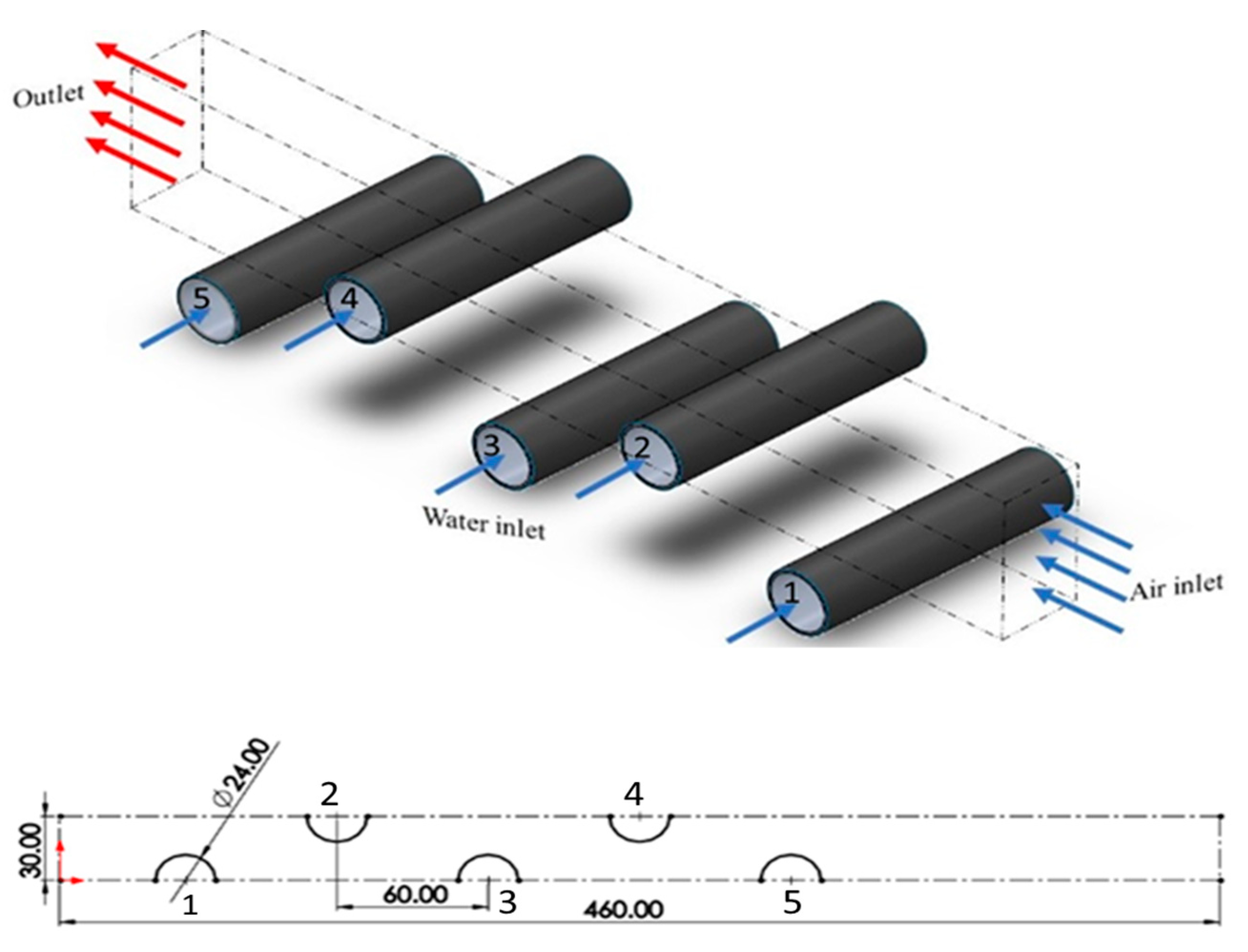
Figure 2. Temperature [K] profile for conditions of case 2 presented in Table 1.

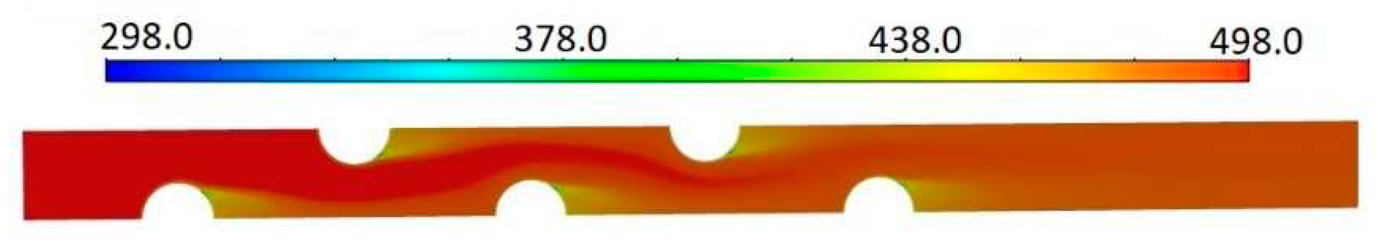
Figure 3. The total heat flux (normalized by pipes' total surface area) versus Re number (a) and the heat transfer coefficient of the last tube (#5) versus Re number (b).

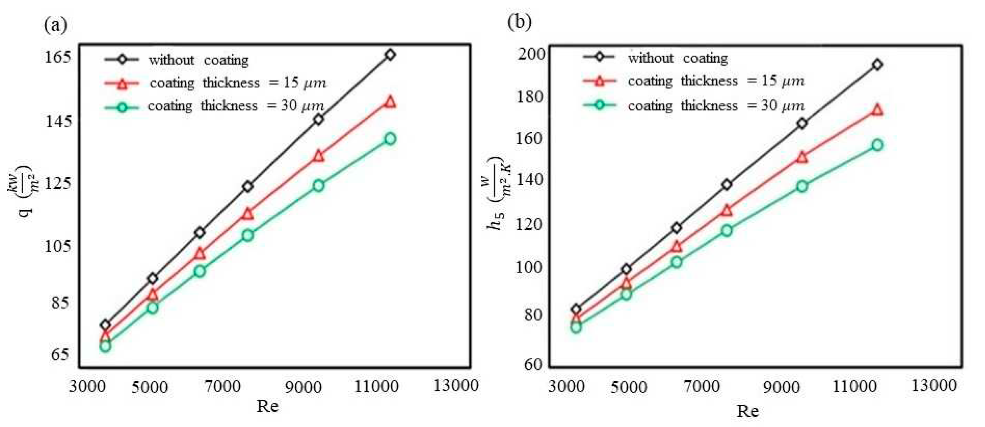
Figure 4. Flowchart of preparing machine learning model based on combining important features.

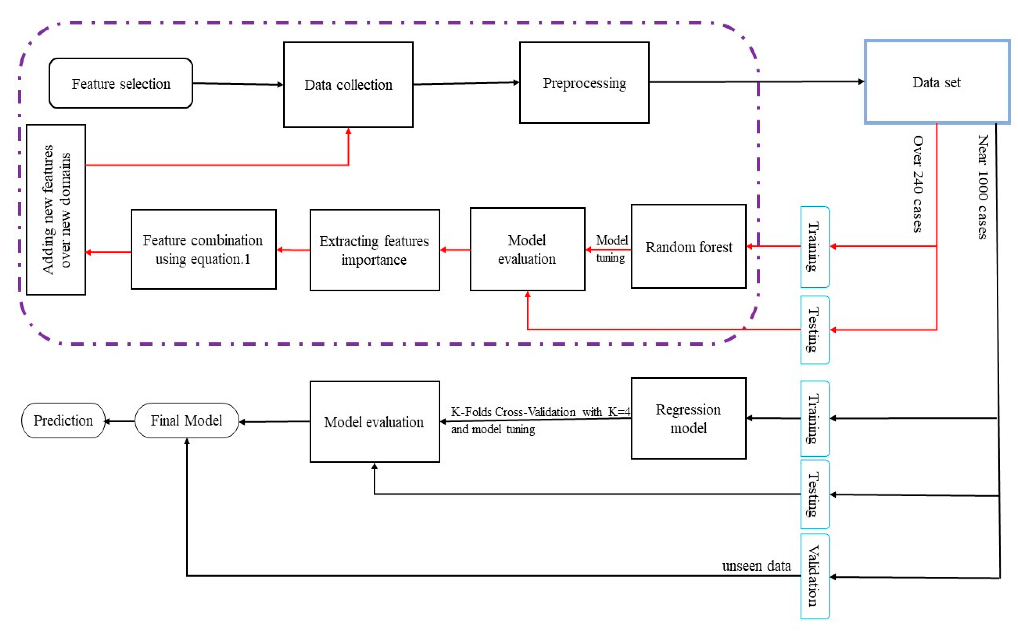
Figure 5. Comparison of predicted total heat flux (q) by FVM simulations and ML regressor.

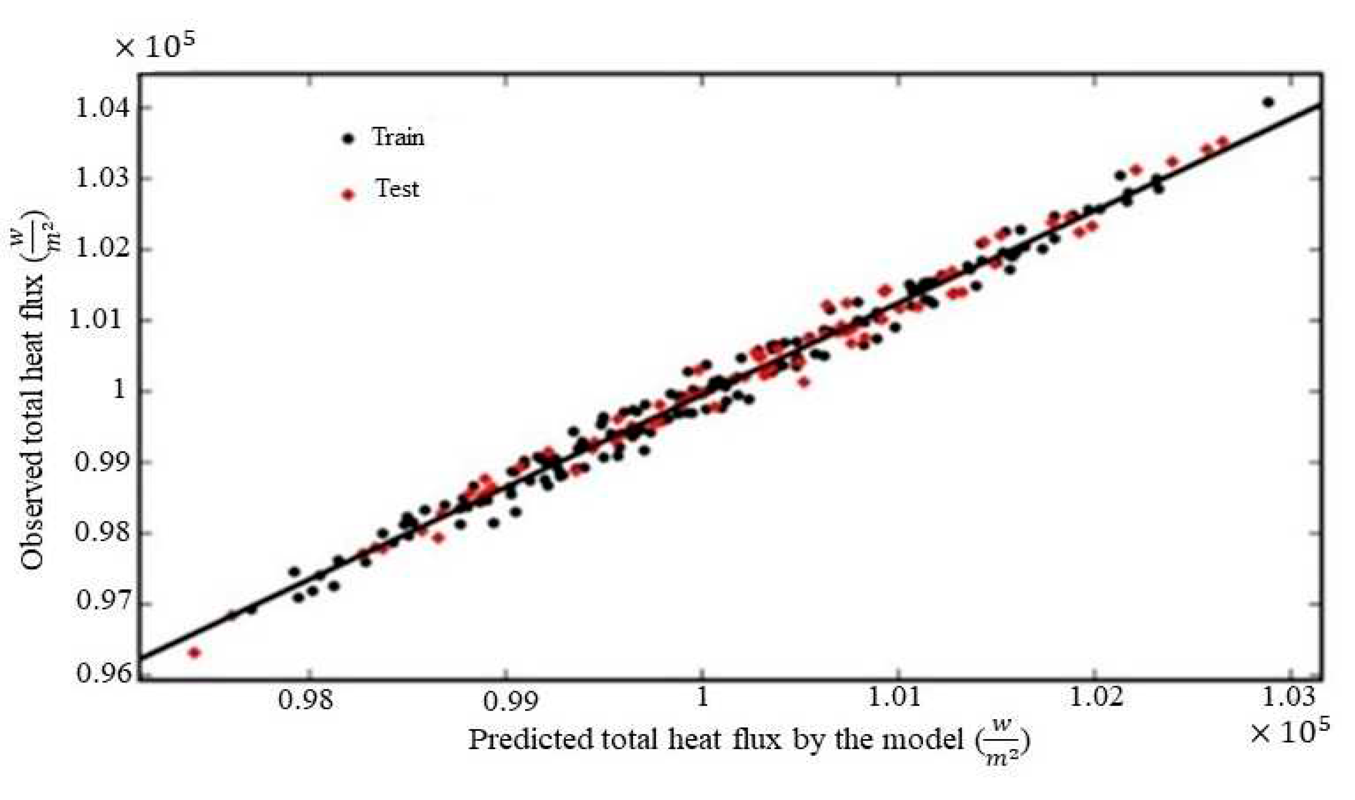
Figure 6. Predictor importance estimation by model.

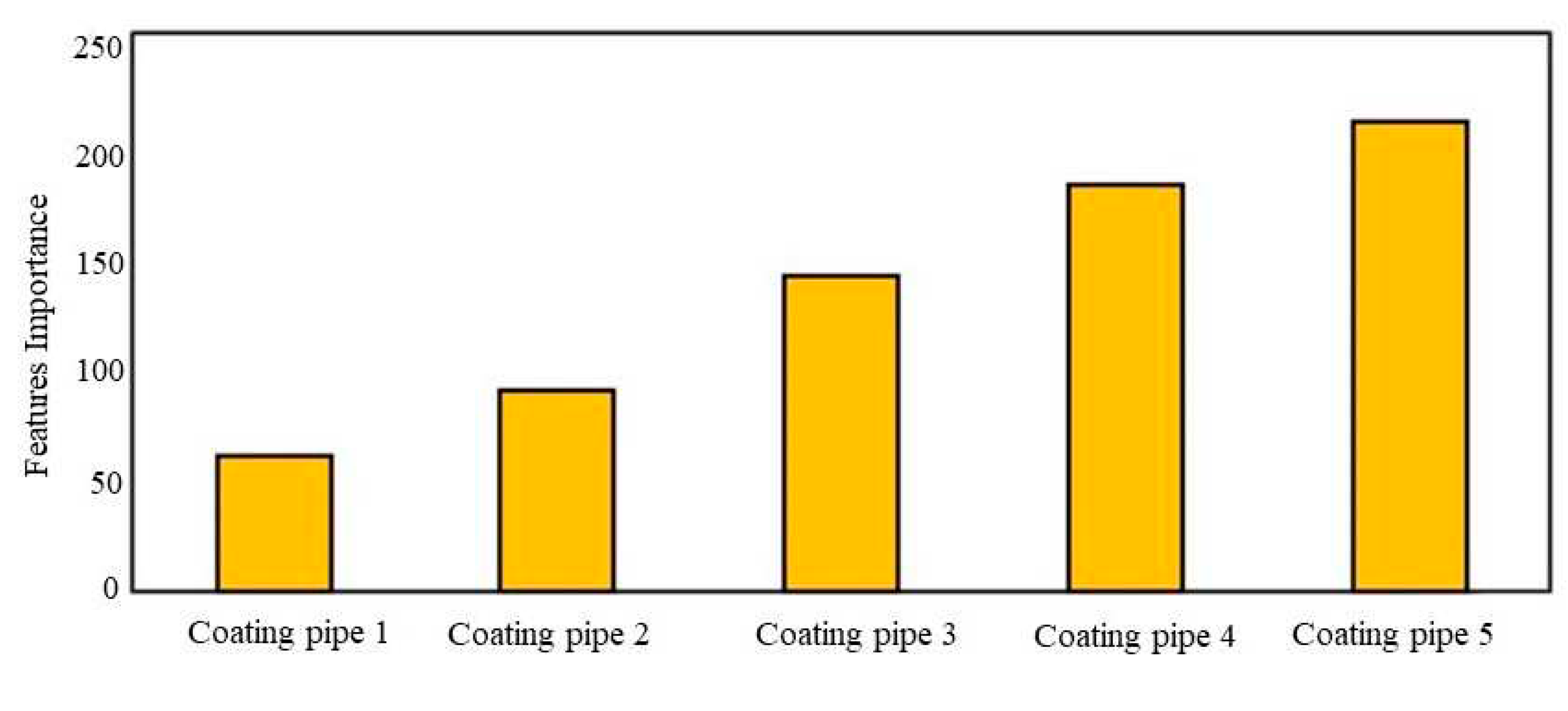
Figure 7. Comparison of the total heat flux (q) calculated by FVM and predicted by random forest after features combination.

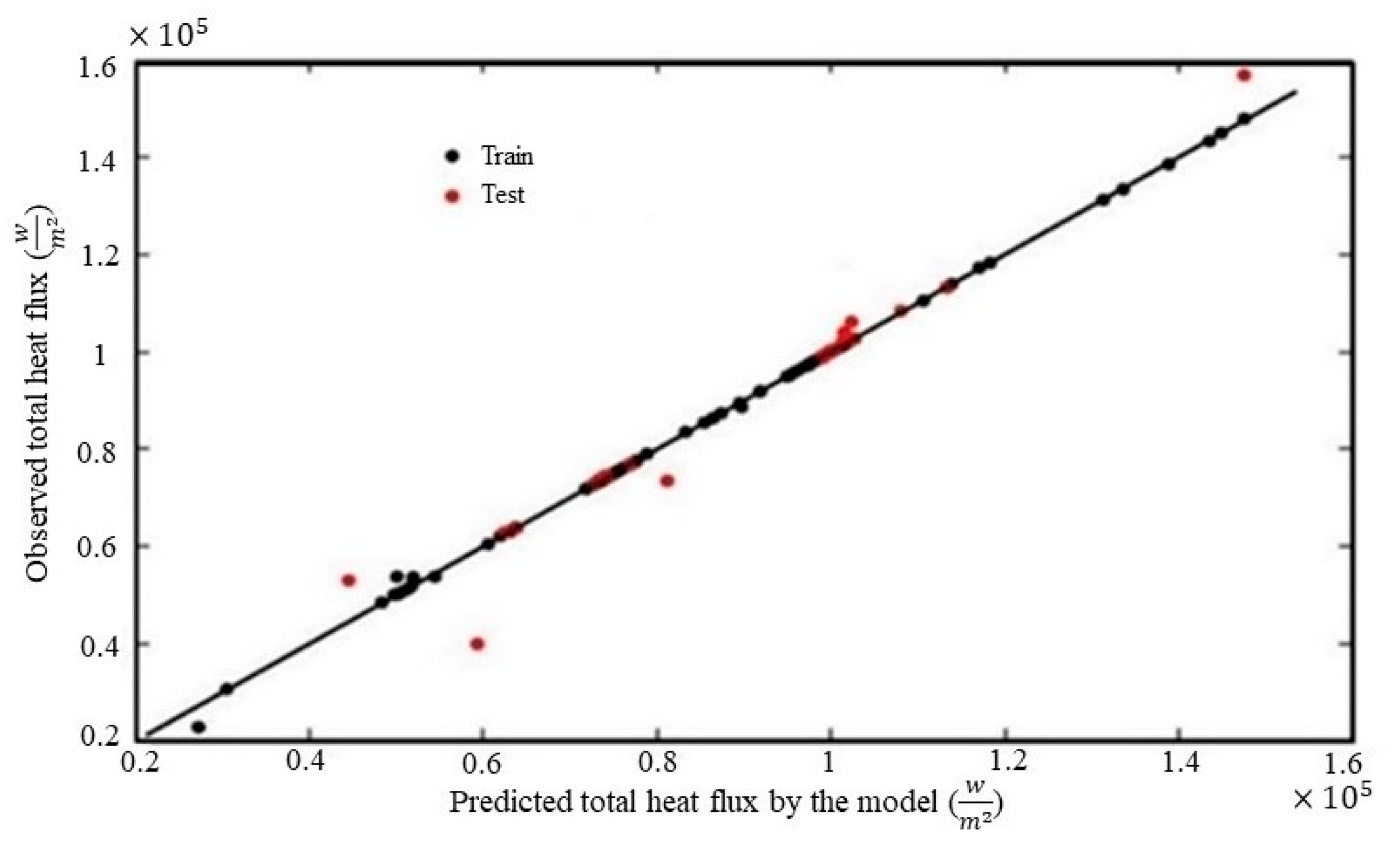
Figure 8. Validating the model with unseen data.

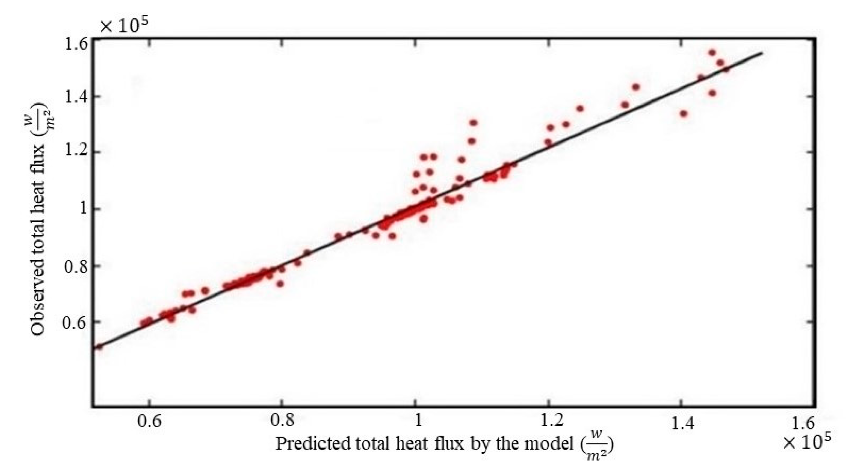
Table 1. Numerical results of different case studies without coating (cases 1 to 3) and with coating (case 4). t is the average of five tubes' coating thickness. The inlet gas has different velocity (V_in) and temperature (T_in) and (

∆ T_{d}

) is the temperature difference between tubes and inlet gas. The last column represents the total heat transfer from tubes wall into the fluid flow.

∆ T_{d}

) is the temperature difference between tubes and inlet gas. The last column represents the total heat transfer from tubes wall into the fluid flow.

Case	t (μm)	$Vin (\frac{m}{s^{2}})$	Tin(K)	∆Td(K)	$q_{t o t a l} (\frac{w}{m^{2}})$
1	---	10	498	200	108599
2	---	10	508	200	108599
3	---	15	498	200	144887
4	30	10	498	200	96316

Table 2. Optimization results with Bayesian approach before features combination.

Tuning hyperparameters
Method	Total trees	Learn rate	Min. Leaf size
L.S.Boost	409	0.49	2

Table 3. Optimization results with Bayesian approach after features combination.

Tuning hyperparameters
Method	Total trees	Learn rate	Min. Leaf size	Max. Num. Splits	Num. Variables to sample
L.S.Boost	202	0.132	4	18	3

Table 4. The total heat flux calculated for different coating thickness.

[t₁ , t₂ , t₃ , t₄ , t₅]	t_average	$Total heat flux \frac{w}{m^{2}}$
[20,20,20,20,20]	20	100020
[100,0,0,0,0]	20	104066
[0,0,0,0,100]	20	100685
[30,30,20,10,10]	20	100940

Table 5. Comparison of all models R².

	Methods
	Feature combination with equation1	Without feature combination
Models	${(R}_{t r a i n}^{2}, R_{u n s e e n d a t a}^{2})$	${(R}_{t r a i n}^{2}, R_{u n s e e n d a t a}^{2})$
Random forest	(0.9994, 0.9810)	(0.9979,0.9732)
K-Nearest Neighbors	(1.0, 0.9037)	(1.0, 0.5390)
Support Vector Regression	(0.9995, 0.9754)	(0.9995, 0.9489)

Disclaimer/Publisher’s Note: The statements, opinions and data contained in all publications are solely those of the individual author(s) and contributor(s) and not of MDPI and/or the editor(s). MDPI and/or the editor(s) disclaim responsibility for any injury to people or property resulting from any ideas, methods, instructions or products referred to in the content.

© 2023 by the authors. Licensee MDPI, Basel, Switzerland. This article is an open access article distributed under the terms and conditions of the Creative Commons Attribution (CC BY) license (http://creativecommons.org/licenses/by/4.0/).

Copyright: This open access article is published under a Creative Commons CC BY 4.0 license, which permit the free download, distribution, and reuse, provided that the author and preprint are cited in any reuse.

Downloads

123

Views

Comments

Subscription

Notify me about updates to this article or when a peer-reviewed version is published.

MDPI Initiatives

Important Links

Choose an area of interest and we will send you notifications of new preprints at your preferred frequency.

Disclaimer