Submitted:
25 May 2023
Posted:
29 May 2023
You are already at the latest version
Abstract
Keywords:
1. Introduction
2. Materials and Methods
2.1. Study Area Description
2.2. Data sources and acquisition
2.3. Trend analysis
2.4. Cross Correlation analysis
2.5. Autocorrelation Analysis
2.6. Gradient Boosting Regression
2.7. Performance Criteria
3. Results and Discussions
3.1. Trend Analysis
3.2. Cross correlations
3.3. Autocorrelations
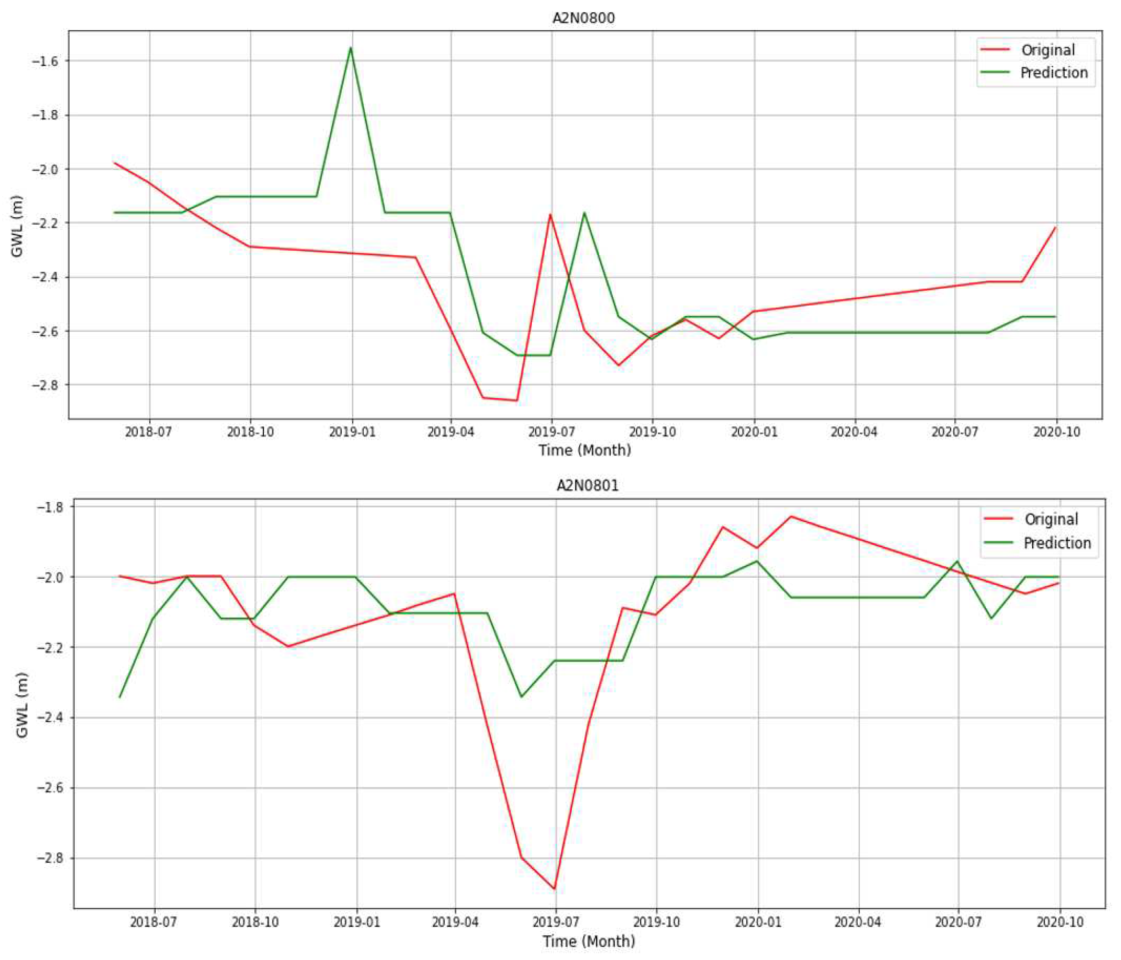
3.4. Gradient Boosting Regression Results
4. Conclusions and Recommendations
References
- Abiye, T. A. , Mengistu, H., Masindi, K., & Demlie, M. (2015). Surface Water and Groundwater Interaction in the Upper Crocodile River Basin, Johannesburg, South Africa: Environmental Isotope Approach. South African Journal of Geology 118, 109–118. [CrossRef]
- Aderemi, B. A. , Olwal, T. O., Ndambuki, J. M. M., & Rwanga, S. S. (2022). Groundwater Levels Forecasting Using Machine Learning Models: A Case Study of the Groundwater Region 10 at Karst Belt, South Africa. SSRN Electronic Journal 200049. [CrossRef]
- Ahmadi, A. , Olyaei, M., Heydari, Z., Emami, M., Zeynolabedin, A., Ghomlaghi, A., Daccache, A., Fogg, G. E., & Sadegh, M. (2022). Groundwater Level Modeling with Machine Learning: A Systematic Review and Meta-Analysis. Water (Switzerland) 14, 1–22. [CrossRef]
- Alfaro, P. , Liesch, T., & Goldscheider, N. (2017). Modélisation de la surexploitation des eaux souterraines dans le Sud de la Vallée du Jourdain avec peu de données. Hydrogeology Journal 25, 13419–1340. [CrossRef]
- Alhaji, U. U. , Yusuf, A. S., Edet, C. O., Oche, C. O., & Agbo, E. P. (2018). Trend Analysis of Temperature in Gombe State Using Mann Kendall Trend Test. Journal of Scientific Research and Reports 20(3), 1–9. [CrossRef]
- Archer, E. , du Toit, J., Engelbrecht, C., Hoffman, M. T., Landman, W., Malherbe, J., & Stern, M. (2022). The 2015-19 multi year drought in the Eastern Cape, South Africa: it’s evolution and impacts on agriculture. Journal of Arid Environments 196, 104630. [CrossRef]
- Bloomfield, J. P. , Allen, D. J., & Griffiths, K. J. (2009). Examining geological controls on baseflow index (BFI) using regression analysis: An illustration from the Thames Basin, UK. Journal of Hydrology 373, 164–176. [CrossRef]
- Bopape, M. J. M. , Sebego, E., Ndarana, T., Maseko, B., Netshilema, M., Gijben, M., Landman, S., Phaduli, E., Rambuwani, G., van Hemert, L., & Mkhwanazi, M. (2021). Evaluating south african weather service information on idai tropical cyclone and kwazulu-natal flood events. South African Journal of Science 117, 1–13. [CrossRef]
- Caren, M. , & Pavlić, K. (2021). Autocorrelation and cross-correlation flow analysis along the confluence of the kupa and sava rivers. Rudarsko Geolosko Naftni Zbornik 36, 67–77. [CrossRef]
- Castellazzi, P. , Longuevergne, L., Martel, R., Rivera, A., Brouard, C., & Chaussard, E. (2018). Quantitative mapping of groundwater depletion at the water management scale using a combined GRACE/InSAR approach. Remote Sensing of Environment 205, 408–418. [CrossRef]
- Centre for Research on the Epidemiology of Disasters. (2023). Disasters in numbers 2022.
- Chandrasekara, S. S. K. , Kwon, H. H., Vithanage, M., Obeysekera, J., & Kim, T. W. (2021). Drought in south asia: A review of drought assessment and prediction in south asian countries. Atmosphere 12. [CrossRef]
- Condon, L. E. , Kollet, S., Bierkens, M. F. P., Fogg, G. E., Maxwell, R. M., Hill, M. C., Fransen, H. J. H., Verhoef, A., Van Loon, A. F., Sulis, M., & Abesser, C. (2021). Global Groundwater Modeling and Monitoring: Opportunities and Challenges. Water Resources Research 57, 1–27. [CrossRef]
- Denić-Jukić, V. , Lozić, A., & Jukić, D. (2020). An application of correlation and spectral analysis in hydrological study of neighboring karst springs. Water (Switzerland) 12. [CrossRef]
- Dilawar, A. , Chen, B., Arshad, A., Guo, L., Ehsan, M. I., Hussain, Y., Kayiranga, A., Measho, S., Zhang, H., Wang, F., Sun, X., & Ge, M. (2021). Towards understanding variability in droughts in response to extreme climate conditions over the different agro-ecological zones of Pakistan. Sustainability (Switzerland) 13. [CrossRef]
- DWAF. (2004). Crocodile River (West) and Marico Water Management Area: Internal Strategic Perspective of the Crocodile River (West) Catchment. Department of Water Affairs and Forestry, South Africa 03/000/00/, 160.
- Géron, A. (2019). Hands-on Machine Learning whith Scikit-Learing, Keras and Tensorfow. In O’Reilly Media, Inc.
- Gude, V. G. , & Nirmalakhandan, N. (2009). Desalination at low temperatures and low pressures. Desalination 244, 239–247. [CrossRef]
- Gyamfi, C. , Ndambuki, J. M., & Salim, R. W. (2016). A Historical Analysis of Rainfall Trend in the Olifants Basin in South Africa. Earth Science Research 5(1), 129. [CrossRef]
- Holmes, M. , Campbell, E. E., Wit, M. De, & Taylor, J. C. (2022). South African Journal of Botany The impact of drought in the Karoo - revisiting diatoms as water quality indicators in the upper reaches of the Great Fish River, Eastern Cape, South Africa. South African Journal of Botany 149, 502–510. [CrossRef]
- Hussain, M. , Butt, A. R., Uzma, F., Ahmed, R., Irshad, S., Rehman, A., & Yousaf, B. (2020). A comprehensive review of climate change impacts, adaptation, and mitigation on environmental and natural calamities in Pakistan. Environmental Monitoring and Assessment 192. [CrossRef]
- Hussein, E. A. , Thron, C., Ghaziasgar, M., Bagula, A., & Vaccari, M. (2020). Groundwater prediction using machine-learning tools. Algorithms 13, 1–16. [CrossRef]
- Ibrahem Ahmed Osman, A. , Najah Ahmed, A., Chow, M. F., Feng Huang, Y., & El-Shafie, A. (2021). Extreme gradient boosting (Xgboost) model to predict the groundwater levels in Selangor Malaysia. Ain Shams Engineering Journal 12(2), 1545–1556. [CrossRef]
- IPCC:2014. (2014). Climate Change 2014: Impacts, Adaptation, and Vulnerability. BMJ (Online) 349. [CrossRef]
- Kanyama, Y. (2021). Application of machine learning techniques in predicting groundwater levels and discharge rates in the North West aquifers.
- Kanyama, Y. , Ajoodha, R., Seyler, H., Makondo, N., & Tutu, H. (2020). Application of Machine Learning Techniques in Forecasting Groundwater Levels in the Grootfontein Aquifer. 2020 2nd International Multidisciplinary Information Technology and Engineering Conference, IMITEC 2020. [CrossRef]
- Liu, J. (2011). Water Ethics and Water Resource Management - UNESCO Bangkok Regional Unit for Social and Human Sciences in Asia and the Pacific. Available online: http://unesdoc.unesco.org/images/0019/001922/192256E.pdf.
- Lyazidi, R. , Hessane, M. A., Moutei, J. F., & Bahir, M. (2020). Developing a methodology for estimating the groundwater levels of coastal aquifers in the Gareb-Bourag plains, Morocco embedding the visual MODFLOW techniques in groundwater modeling system. Groundwater for Sustainable Development 11, 100471. [CrossRef]
- Madzivhandila, Thanyani S, Maserumule, M. H. (2022). The Irony of A “Fire Fighting” Approach Towards Natural Hazards in South Africa: Lessons From Flooding Disaster in KwaZulu-Natal. Journal of Public Administration 57, 191–194.
- Malekzadeh, M. , Kardar, S., & Shabanlou, S. (2019). Simulation of groundwater level using MODFLOW, extreme learning machine and Wavelet-Extreme Learning Machine models. Groundwater for Sustainable Development 9, 100279. [CrossRef]
- Mann, H. B. (1945). Non-Parametric Test Against Trend. Econometrica 13, 245–259. [CrossRef]
- Mathivha, F. I. , Nkosi, M., & Mutoti, M. I. (2021). Evaluating the relationship between hydrological extremes and groundwater in Luvuvhu River Catchment, South Africa. Journal of Hydrology: Regional Studies 37, 100897. [CrossRef]
- Meyer, M. (2014). Hydrogeology of Groundwater Region 10: The Karst Belt (WRC Project No. K5/1916).
- Mishra, A. K. , & Singh, V. P. (2010). A review of drought concepts. Journal of Hydrology 391, 202–216. [CrossRef]
- Mohan, C. , Western, A. W., Wei, Y., & Saft, M. (2018). Predicting groundwater recharge for varying land cover and climate conditions-a global meta-study. Hydrology and Earth System Sciences 22, 2689–2703. [CrossRef]
- Murdoch, W. J. , Singh, C., Kumbier, K., Abbasi-Asl, R., & Yu, B. (2019). Definitions, methods, and applications in interpretable machine learning. Proceedings of the National Academy of Sciences of the United States of America 116(44), 22071–22080. [CrossRef]
- Oke, S. A. , & Fourie, F. (2017). Guidelines to groundwater vulnerability mapping for Sub-Saharan Africa. Groundwater for Sustainable Development 5, 168–177. [CrossRef]
- Olanrewaju, C. C. , & Reddy, M. (2022). Assessment and prediction of flood hazards using standardized precipitation index—A case study of eThekwini metropolitan area. Journal of Flood Risk Management 15, 1–12. [CrossRef]
- Osman, A. I. A. , Ahmed, A. N., Huang, Y. F., Kumar, P., Birima, A. H., Sherif, M., Sefelnasr, A., Ebraheemand, A. A., & El-Shafie, A. (2022). Past, Present and Perspective Methodology for Groundwater Modeling-Based Machine Learning Approaches. Archives of Computational Methods in Engineering 29, 3843–3859. [CrossRef]
- Ostad-Ali-Askari, K. , Ghorbanizadeh Kharazi, H., Shayannejad, M., & Zareian, M. J. (2019). Effect of management strategies on reducing negative impacts of climate change on water resources of the Isfahan–Borkhar aquifer using MODFLOW. River Research and Applications 35, 611–631. [CrossRef]
- Ouali, L. , Kabiri, L., Namous, M., Hssaisoune, M., Abdelrahman, K., Fnais, M. S., Kabiri, H., El Hafyani, M., Oubaassine, H., Arioua, A., & Bouchaou, L. (2023). Spatial Prediction of Groundwater Withdrawal Potential Using Shallow, Hybrid, and Deep Learning Algorithms in the Toudgha Oasis, Southeast Morocco. Sustainability (Switzerland) 15. [CrossRef]
- Prodhan, F. A. , Zhang, J., Pangali Sharma, T. P., Nanzad, L., Zhang, D., Seka, A. M., Ahmed, N., Hasan, S. S., Hoque, M. Z., & Mohana, H. P. (2022). Projection of future drought and its impact on simulated crop yield over South Asia using ensemble machine learning approach. Science of the Total Environment 807, 151029. [CrossRef]
- Qi, P. , Zhang, G., Xu, Y. J., Wang, L., Ding, C., & Cheng, C. (2018). Assessing the influence of precipitation on shallow groundwater table response using a combination of singular value decomposition and cross-wavelet approaches. Water (Switzerland) 10. [CrossRef]
- Quesada-Román, A. , Villalobos-Portilla, E., & Campos-Durán, D. (2020). Hydrometeorological disasters in urban areas of Costa Rica, Central America. Environmental Hazards 1–15. [CrossRef]
- Rahmani, F. , & Fattahi, M. H. (2021). A multifractal cross-correlation investigation into sensitivity and dependence of meteorological and hydrological droughts on precipitation and temperature. Natural Hazards 109, 2197–2219. [CrossRef]
- Rezaei, M. , Mousavi, S. F., Moridi, A., Eshaghi Gordji, M., & Karami, H. (2021). A new hybrid framework based on integration of optimization algorithms and numerical method for estimating monthly groundwater level. Arabian Journal of Geosciences 14. [CrossRef]
- Sahoo, M. , Kasot, A., Dhar, A., & Kar, A. (2018). On Predictability of Groundwater Level in Shallow Wells Using Satellite Observations. Water Resources Management 32(4), 1225–1244. [CrossRef]
- Schreiner, B. G. , Mungatana, E. D., & Baleta, H. (2018). Impacts of Drought Induced Water Shortages in South Africa: Economic Analysis Report to the Water Research Commission. 2604, pp. 1–85. Available online: www.wrc.org.za.
- Schulze, R. E. (2012). A 2011 Perspective On Climate Change And The South African Water Sector. In WRC Report No. TT 518/12. Available online: http://www.wrc.org.za/wp-content/uploads/mdocs/TT 518-12.pdf.
- Seo, S. B. , Das Bhowmik, R., Sankarasubramanian, A., Mahinthakumar, G., & Kumar, M. (2019). The role of cross-correlation between precipitation and temperature in basin-scale simulations of hydrologic variables. Journal of Hydrology 570, 304–314. [CrossRef]
- Sharafati, A. , Asadollah, S. B. H. S., & Neshat, A. (2020a). A new artificial intelligence strategy for predicting the groundwater level over the Rafsanjan aquifer in Iran. Journal of Hydrology 591, 125468. [CrossRef]
- Sharafati, A. , Asadollah, S. B. H. S., & Neshat, A. (2020b). A new artificial intelligence strategy for predicting the groundwater level over the Rafsanjan aquifer in Iran. Journal of Hydrology 591, 125468. [CrossRef]
- Sokol, Z. , & Bližňák, V. (2009). Areal distribution and precipitation-altitude relationship of heavy short-term precipitation in the Czech Republic in the warm part of the year. Atmospheric Research 94, 652–662. [CrossRef]
- Sun, H. , & Cornish, P. S. (2005). Estimating shallow groundwater recharge in the headwaters of the Liverpool Plains using SWAT. Hydrological Processes 19(3), 795–807. [CrossRef]
- Valois, R. , MacDonell, S., Núñez Cobo, J. H., & Maureira-Cortés, H. (2020). Groundwater level trends and recharge event characterization using historical observed data in semi-arid Chile. Hydrological Sciences Journal 65, 597–609. [CrossRef]
- Van Loon, A. F. , Kumar, R., & Mishra, V. (2017). Testing the use of standardised indices and GRACE satellite data to estimate the European 2015 groundwater drought in near-real time. Hydrology and Earth System Sciences 21, 1947–1971. [CrossRef]
- Wanders, N. , Wada, Y., & Van Lanen, H. A. J. (2015). Global hydrological droughts in the 21st century under a changing hydrological regime. Earth System Dynamics 6(1), 1–15. [CrossRef]
- Wei, A. , Chen, Y., Li, D., Zhang, X., Wu, T., & Li, H. (2022). Prediction of groundwater level using the hybrid model combining wavelet transform and machine learning algorithms. Earth Science Informatics 15(3), 1951–1962. [CrossRef]
- Xu, Y. , & Beekman, H. E. (2019). Review: Groundwater recharge estimation in arid and semi-arid southern Africa. Hydrogeology Journal 27, 929–943. [CrossRef]
- Zeydalinejad, N. (2022). Artificial neural networks vis-à-vis MODFLOW in the simulation of groundwater: a review. Modeling Earth Systems and Environment 8, 2911–2932. [CrossRef]
- Ziervogel, G. , New, M., Archer van Garderen, E., Midgley, G., Taylor, A., Hamann, R., Stuart-Hill, S., Myers, J., & Warburton, M. (2014). Climate change impacts and adaptation in South Africa. Wiley Interdisciplinary Reviews: Climate Change 5, 605–620. [CrossRef]
- Zomlot, Z. , Verbeiren, B., Huysmans, M., & Batelaan, O. (2015). Spatial distribution of groundwater recharge and base flow: Assessment of controlling factors. Journal of Hydrology: Regional Studies 4, 349–368. [CrossRef]
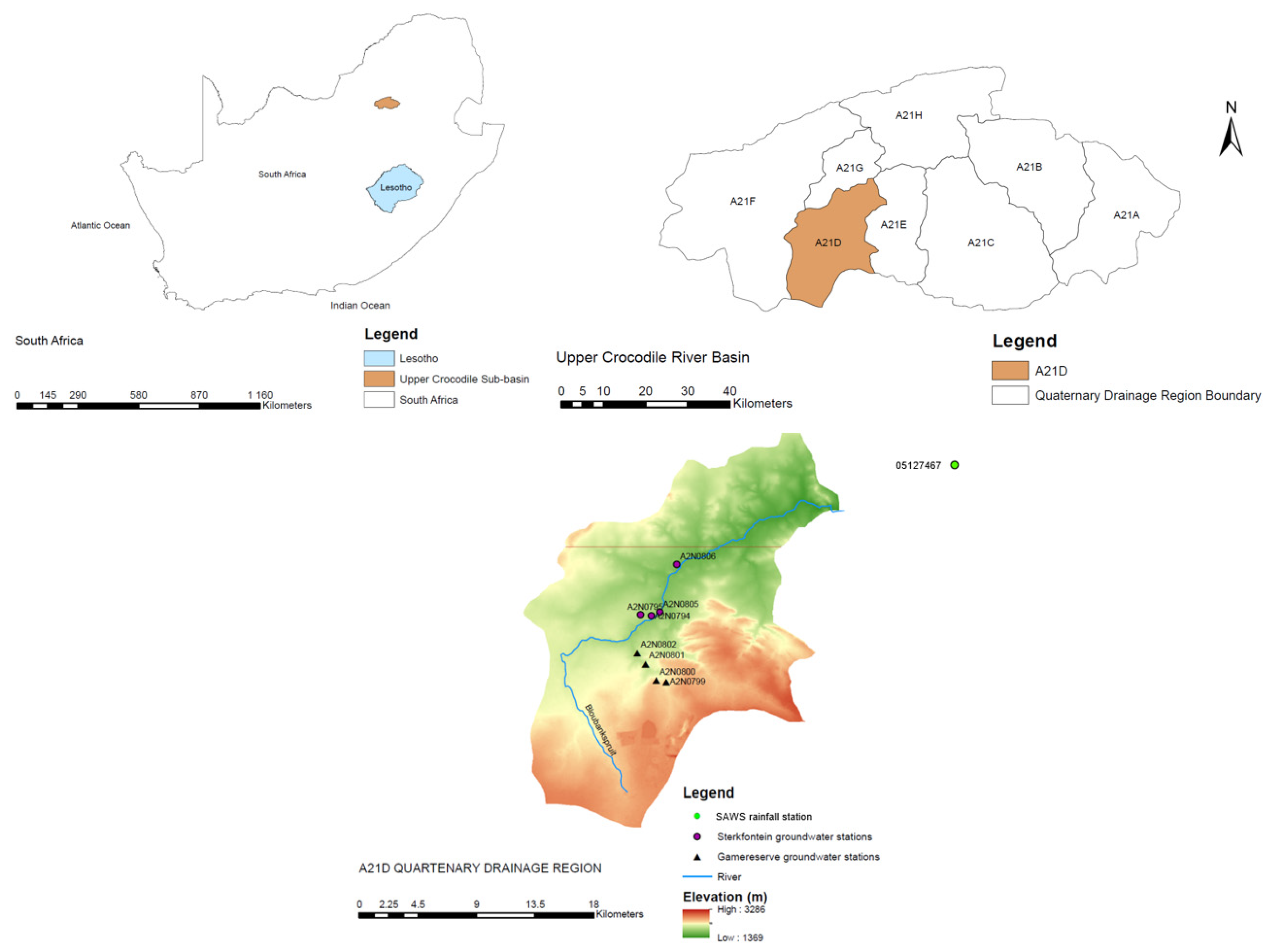
| STATION NUMBER | LATITUDE | LONGITUDE | START DATE | QUATERNARY |
|---|---|---|---|---|
| A2N0794 | -26.048 | 27.709 | 01/09/2008 | A21D |
| A2N0795 | -26.047 | 27.702 | 01/09/2008 | A21D |
| A2N0799 | -26.093 | 27.719 | 01/09/2008 | A21D |
| A2N0800 | -26.092 | 27.712 | 01/09/2008 | A21D |
| A2N0801 | -26.081 | 27.705 | 01/09/2008 | A21D |
| A2N0802 | -26.073 | 27.699 | 01/09/2008 | A21D |
| A2N0803 | -26.036 | 27.715 | 01/09/2008 | A21D |
| A2N0805 | -26.045 | 27.715 | 01/09/2008 | A21D |
| A2N0806 | -26.012 | 27.727 | 01/09/2008 | A21D |
| Groundwater stations | ||||||||
|---|---|---|---|---|---|---|---|---|
| Parameter | A2N0794 | A2N0795 | A2N0799 | A2N0800 | A2N0801 | A2N0802 | A2N0805 | A2N0806 |
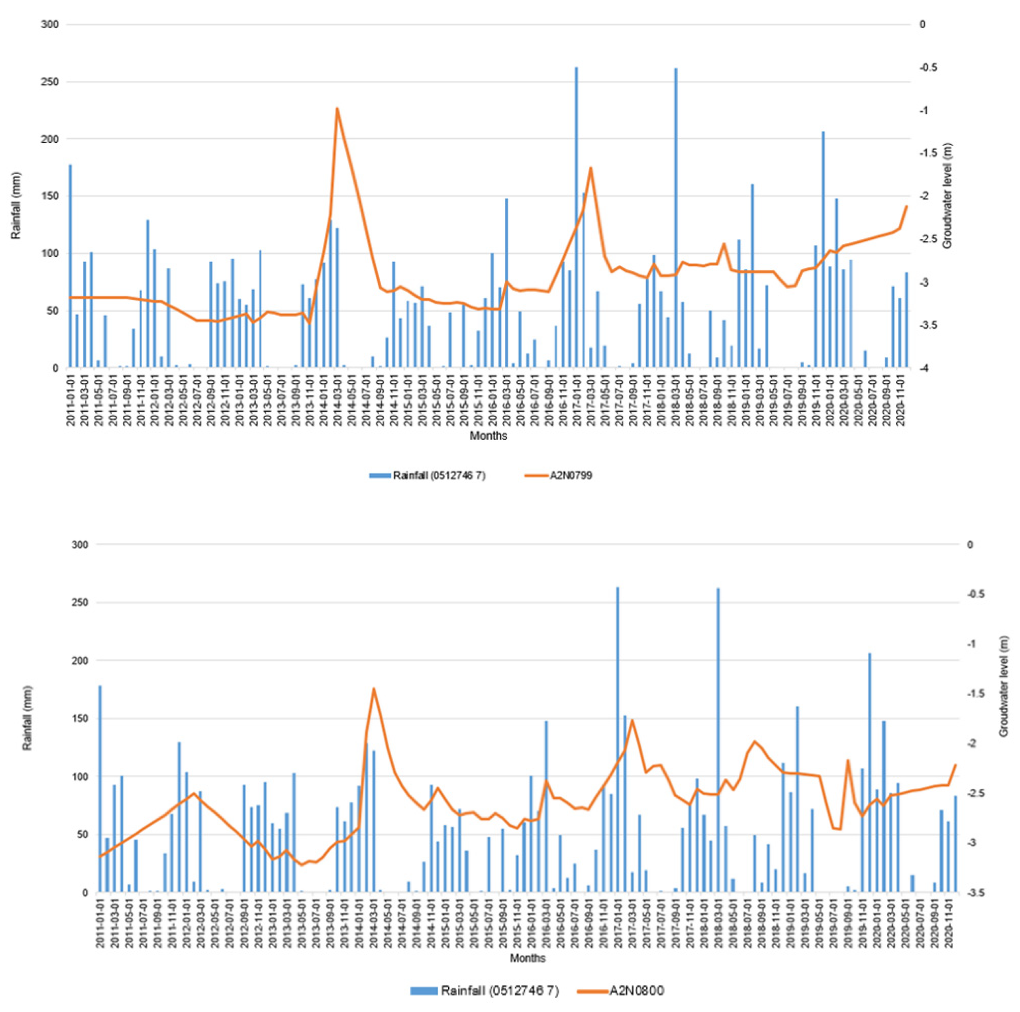
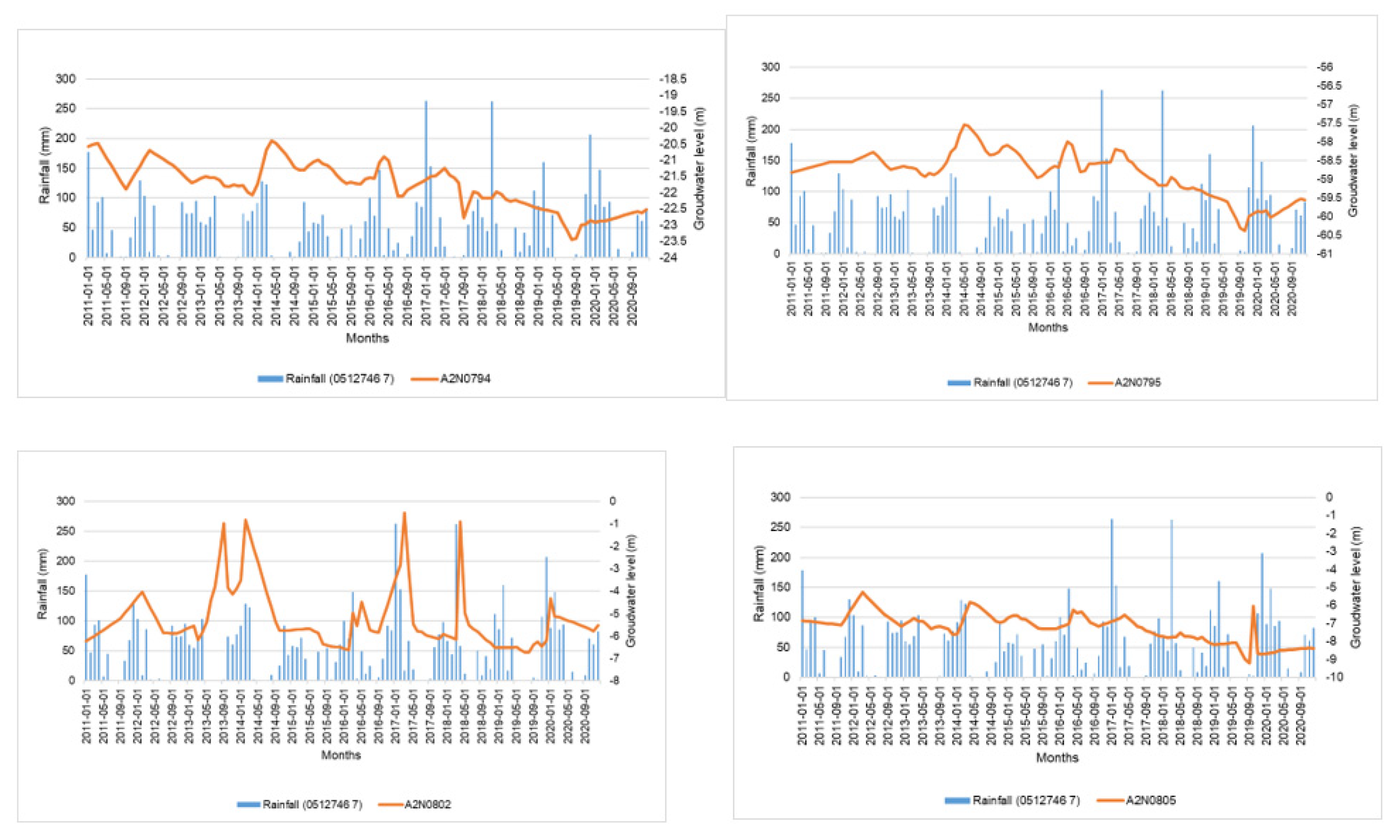
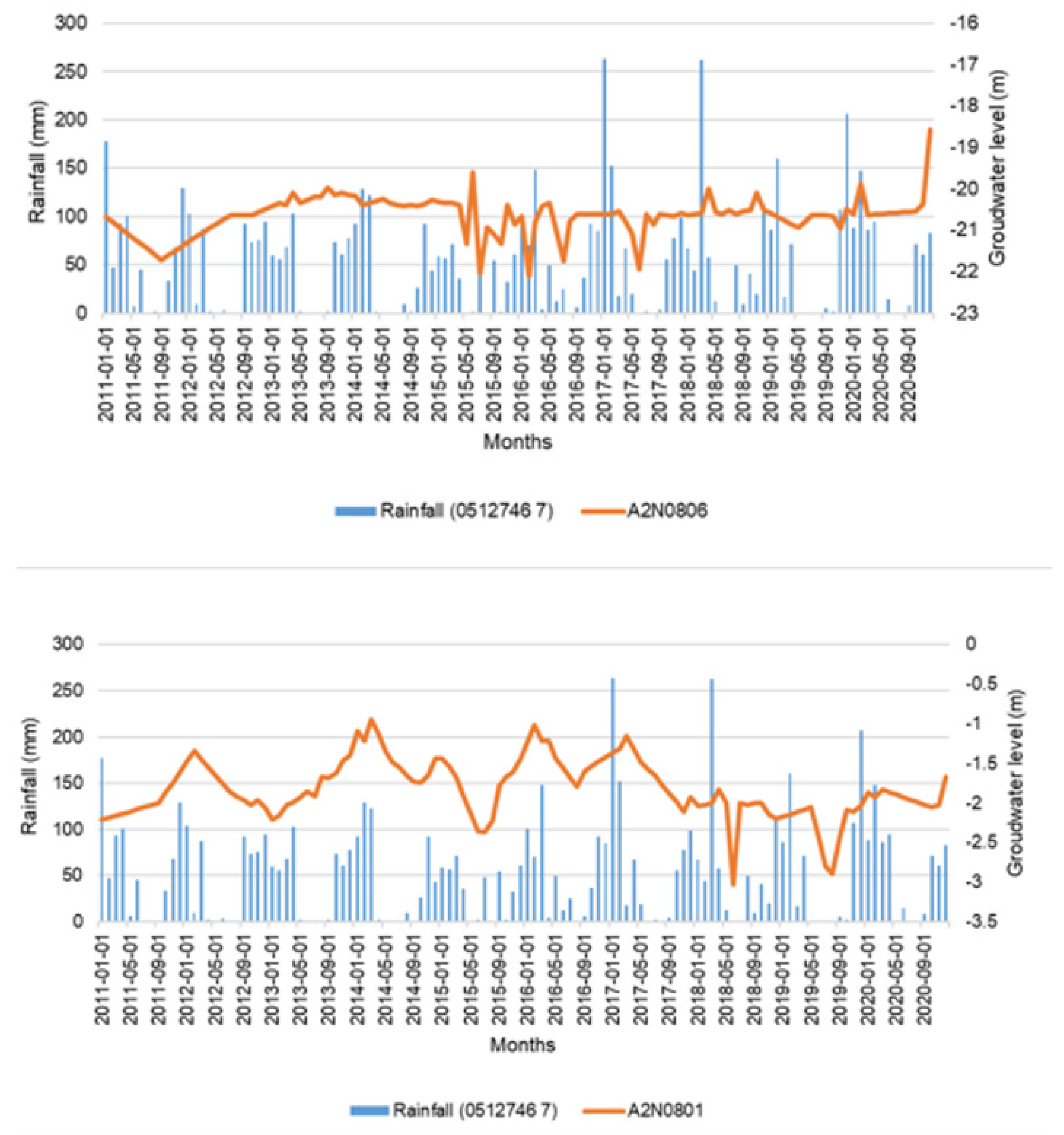
| Trend | Decreasing | Decreasing | Increasing | Increasing | No trend | Decreasing | Decreasing | No trend |
| P-value | 0.000 | 0.000 | 0.000 | 0.000 | 0.055 | 0.001 | 0.000 | 0.133 |
| Z | -9.606 | -7.277 | 7.460 | 6.496 | -1.917 | -3.176 | -8.896 | 1.502 |
| Tau | -0.593 | -0.448 | 0.461 | 0.401 | -0.118 | -0.196 | -0.547 | 0.093 |
| S | -4236.000 | -3249.000 | 3289.000 | 2865.000 | -846.000 | -1401.000 | -3972.000 | 663.000 |
| Var(S) | 194360.000 | 199213.667 | 194262.333 | 194357.000 | 194314.000 | 194361.667 | 199240.000 | 194333.000 |
| Slope | -0.017 | -0.011 | 0.006 | 0.005 | -0.002 | -0.007 | -0.018 | 0.001 |
| STATION | LAG(MONTHS) | CCmax |
|---|---|---|
| A2N0794 | 3 | 0.145 |
| A2N0799 | 2 | 0.288 |
| A2N0800 | 2 | 0.2 |
| A2N0801 | 1 | 0.239 |
| A2N0802 | 1 | 0.299 |
| A2N0806 | 0 | 0.094 |
| A2N0795 | 3 | 0.065 |
| A2N0805 | 3 | 0.097 |
| STATION | LAG (MONTHS) | AUTOCORRELATION |
|---|---|---|
| A2N0794 | 1 | 0.94 |
| A2N0799 | 1 | 0.892 |
| A2N0800 | 1 | 0.865 |
| A2N0801 | 1 | 0.851 |
| A2N0802 | 1 | 0.755 |
| A2N0806 | 1 | 0.417 |
| A2N0795 | 1 | 0.969 |
| A2N0805 | 1 | 0.848 |
| STATION | MSE | R2 |
|---|---|---|
| A2N0794 | 0.41 | 0.51 |
| A2N0799 | 0.12 | 0.5 |
| A2N0800 | 0.06 | 0.66 |
| A2N0801 | 0.04 | 0.62 |
| A2N0802 | 0.51 | 0.01 |
| A2N0806 | 0.13 | 0.05 |
| A2N0795 | 0.53 | 0.33 |
| A2N0805 | 0.83 | 0.53 |
Disclaimer/Publisher’s Note: The statements, opinions and data contained in all publications are solely those of the individual author(s) and contributor(s) and not of MDPI and/or the editor(s). MDPI and/or the editor(s) disclaim responsibility for any injury to people or property resulting from any ideas, methods, instructions or products referred to in the content. |
© 2024 by the authors. Licensee MDPI, Basel, Switzerland. This article is an open access article distributed under the terms and conditions of the Creative Commons Attribution (CC BY) license (https://creativecommons.org/licenses/by/4.0/).


