Submitted:
26 May 2023
Posted:
29 May 2023
You are already at the latest version
Abstract
Keywords:
1. Introduction
2. Related Work
2.1. Semisupervised Action Recognition
2.2. Multiple Feature Analysis
2.3. Embedded Subspace Representation
3. Proposed Approach
3.1. Formulation
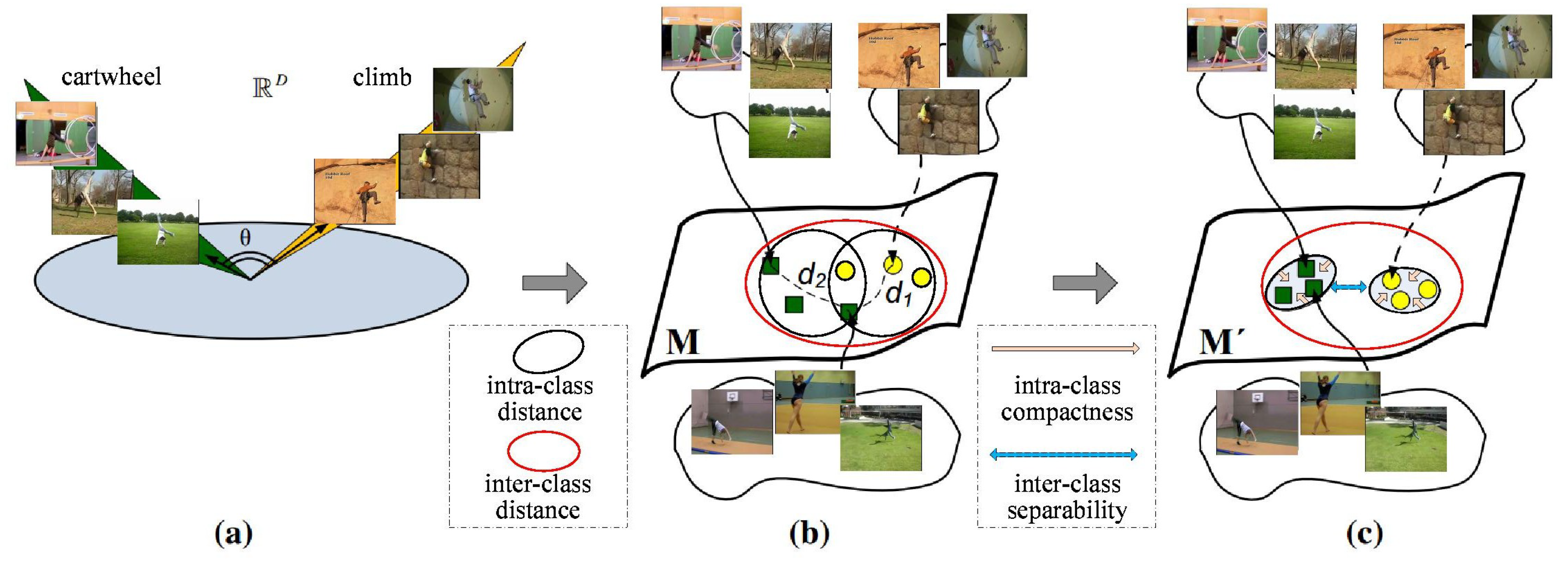
3.2. Manifold Learning
3.3. Multiple Feature Analysis
3.4. Grassmannian Kernels
3.5. Optimisation
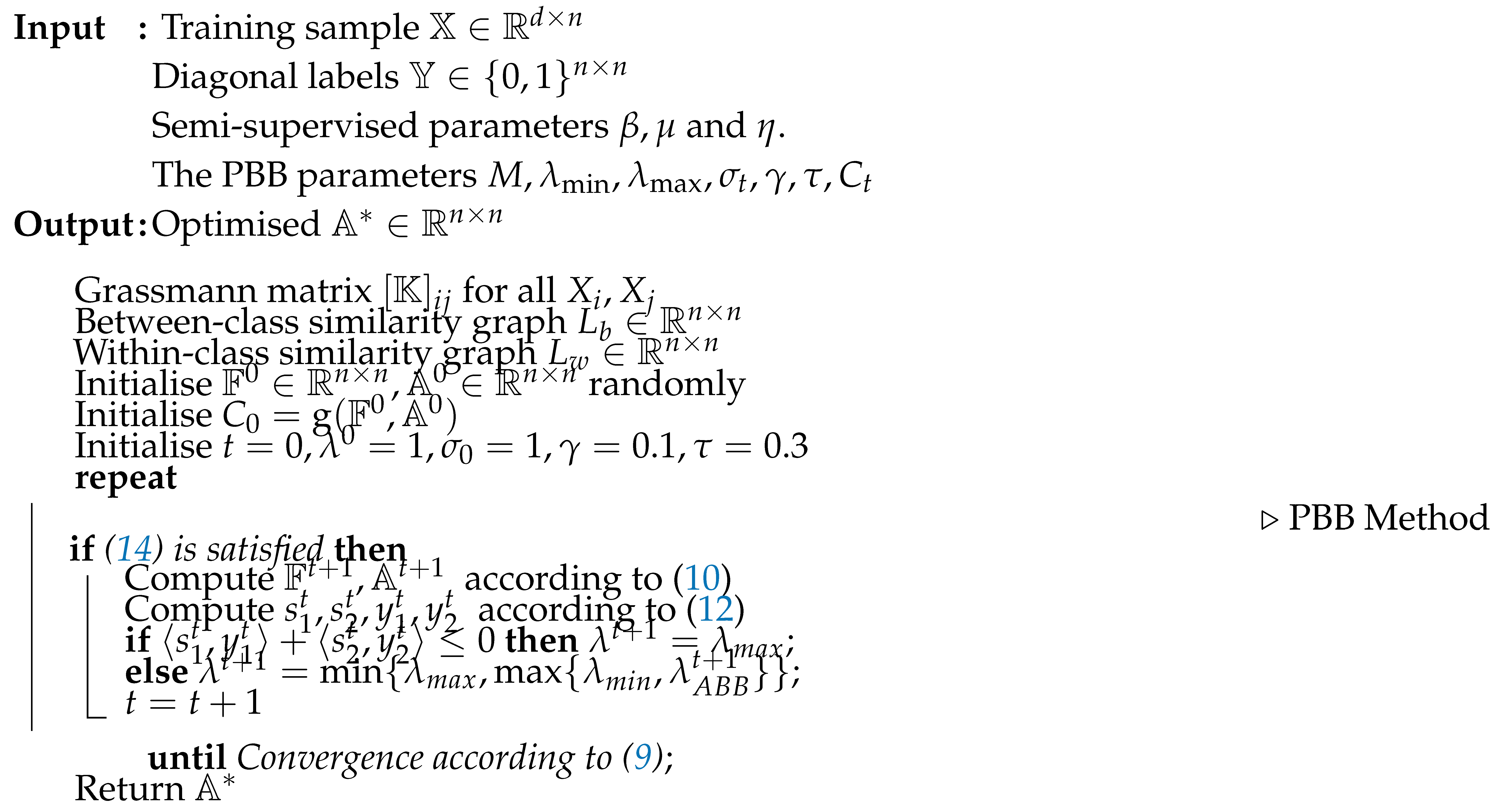
3.6. Projected Barzilai-Borwein
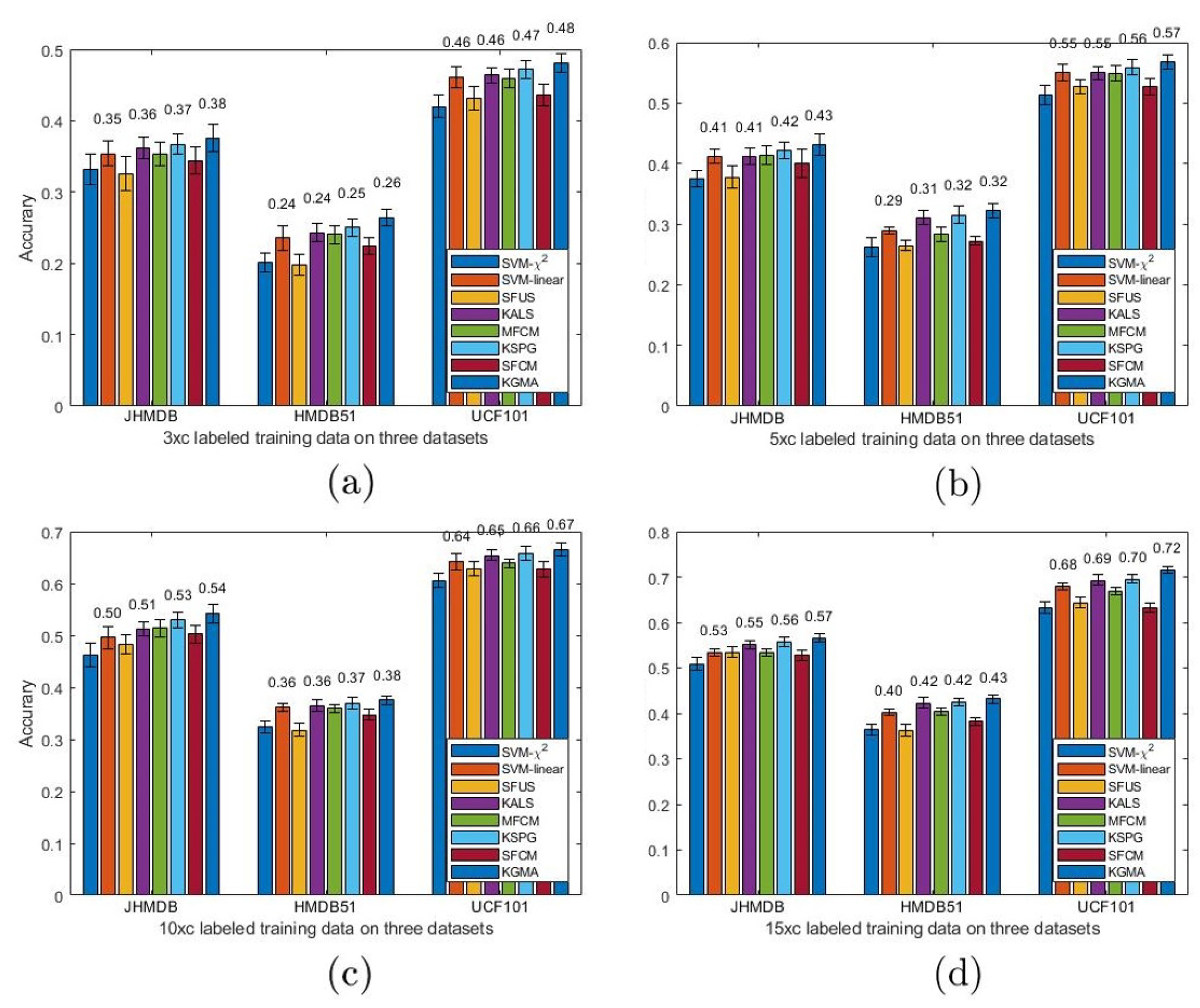
4. Experiments
| JHMDB | HMDB51 | UCF101 | |
|---|---|---|---|
| SFUS | 0.6942 ± 0.0121 | 0.5217 ± 0.0114 | 0.7910 ± 0.0087 |
| SFCM | 0.7125 ± 0.0099 | 0.5394 ± 0.0108 | 0.8070 ± 0.0101 |
| MFCU | 0.7154 ± 0.0088 | 0.5556 ± 0.0098 | 0.8429 ± 0.0085 |
| SVM- | 0.6931 ± 0.0106 | 0.5190 ± 0.0095 | 0.8138 ± 0.0108 |
| SVM-linear | 0.7140 ± 0.0086 | 0.5385 ± 0.0077 | 0.8450 ± 0.0087 |
| KSPG | 0.7287 ± 0.0114 | 0.5697 ± 0.0833 | 0.8552 ± 0.0111 |
| KALS | 0.7218 ± 0.0087 | 0.5607 ± 0.0098 | 0.8411 ± 0.0095 |
| KGMA | 0.7361±0.0096 | 0.5762±0.1040 | 0.8673±0.0087 |
5. Conclusion
References
- Wang, H.; Dan, O.; Verbeek, J.; Schmid, C. A Robust and Efficient Video Representation for Action Recognition. IJCV 2016, 119, 219–238. [Google Scholar] [CrossRef]
- Wang, L.; Xiong, Y.; Wang, Z.; Qiao, Y.; Lin, D.; Tang, X.; Van Gool, L. Temporal segment networks: towards good practices for deep action recognition. ECCV, 2016.
- Wang, S.; Yang, Y.; Ma, Z.; Li, X. Action recognition by exploring data distribution and feature correlation. CVPR, 2012, pp. 1370–1377.
- Wang, S.; Ma, Z.; Yang, Y.; Li, X.; Pang, C.; Hauptmann, A.G. Semi-Supervised Multiple Feature Analysis for Action Recognition. IEEE Transactions on Multimedia 2014, 16, 289–298. [Google Scholar]
- Luo, M.; Chang, X.; Nie, L.; Yang, Y.; Hauptmann, A.G.e.a. An Adaptive Semisupervised Feature Analysis for Video Semantic Recognition. IEEE Transactions on Cybernetics 2018, 48, 648–660. [Google Scholar] [CrossRef] [PubMed]
- Chang, X.; Yang, Y. Semisupervised Feature Analysis by Mining Correlations Among Multiple Tasks. IEEE TNNLS 2017, 28, 2294–2305. [Google Scholar] [CrossRef]
- Liu, H.; Li, X. Modified subspace Barzilai-Borwein gradient method for non-negative matrix factorization. Computational Optimization and Applications 2013, 55, 173–196. [Google Scholar]
- BARZILAI. ; JONATHAN.; BORWEIN.; Jonathan, M. Two-Point Step Size Gradient Methods. Journal of Numerical Analysis 1988, 8, 141–148. [Google Scholar] [CrossRef]
- Harandi, M.T.; Sanderson, C.; Shirazi, S.; Lovell, B.C. Kernel analysis on Grassmann manifolds for action recognition. Pattern Recognition Letters 2013, 34, 1906–1915. [Google Scholar]
- Xu, Z.; Hu, R.; Chen, J.; Chen, C.; Jiang, J.; Li, J.; Li, H. Semisupervised discriminant multimanifold analysis for action recognition. IEEE transactions on neural networks and learning systems 2019, 30, 2951–2962. [Google Scholar] [CrossRef] [PubMed]
- Xiao, J.; Jing, L.; Zhang, L.; He, J.; She, Q.; Zhou, Z.; Yuille, A.; Li, Y. Learning from temporal gradient for semi-supervised action recognition. Proceedings of the IEEE/CVF Conference on Computer Vision and Pattern Recognition, 2022, pp. 3252–3262.
- Xu, Y.; Wei, F.; Sun, X.; Yang, C.; Shen, Y.; Dai, B.; Zhou, B.; Lin, S. Cross-model pseudo-labeling for semi-supervised action recognition. Proceedings of the IEEE/CVF Conference on Computer Vision and Pattern Recognition, 2022, pp. 2959–2968.
- Si, C.; Nie, X.; Wang, W.; Wang, L.; Tan, T.; Feng, J. Adversarial self-supervised learning for semi-supervised 3d action recognition. Computer Vision–ECCV 2020: 16th European Conference, Glasgow, UK, –28, 2020, Proceedings, Part VII 16. Springer, 2020, pp. 35–51. 23 August.
- Singh, A.; Chakraborty, O.; Varshney, A.; Panda, R.; Feris, R.; Saenko, K.; Das, A. Semi-supervised action recognition with temporal contrastive learning. Proceedings of the IEEE/CVF Conference on Computer Vision and Pattern Recognition, 2021, pp. 10389–10399.
- Kumar, A.; Rawat, Y.S. End-to-end semi-supervised learning for video action detection. Proceedings of the IEEE/CVF Conference on Computer Vision and Pattern Recognition, 2022, pp. 14700–14710.
- Bi, Y.; Bai, X.; Jin, T.; Guo, S. Multiple feature analysis for infrared small target detection. IEEE Geoscience and Remote Sensing Letters 2017, 14, 1333–1337. [Google Scholar]
- Shahroudy, A.; Ng, T.T.; Gong, Y.; Wang, G. Deep multimodal feature analysis for action recognition in rgb+ d videos. IEEE transactions on pattern analysis and machine intelligence 2017, 40, 1045–1058. [Google Scholar] [CrossRef] [PubMed]
- Khaire, U.M.; Dhanalakshmi, R. Stability of feature selection algorithm: A review. Journal of King Saud University-Computer and Information Sciences 2022, 34, 1060–1073. [Google Scholar] [CrossRef]
- Wang, S.; Ma, Z.; Yang, Y.; Li, X.; Pang, C.; Hauptmann, A.G. Semi-supervised multiple feature analysis for action recognition. IEEE transactions on multimedia 2013, 16, 289–298. [Google Scholar]
- Chang, X.; Yang, Y. Semisupervised feature analysis by mining correlations among multiple tasks. IEEE transactions on neural networks and learning systems 2016, 28, 2294–2305. [Google Scholar] [CrossRef]
- Huynh-The, T.; Hua, C.H.; Ngo, T.T.; Kim, D.S. Image representation of pose-transition feature for 3D skeleton-based action recognition. Information Sciences 2020, 513, 112–126. [Google Scholar] [CrossRef]
- Harandi, M.T.; Sanderson, C.; Shirazi, S.; Lovell, B.C. Graph embedding discriminant analysis on Grassmannian manifolds for improved image set matching. CVPR, 2011.
- Yan, Y.; Ricci, E.; Subramanian, R.; Liu, G.; Sebe, N. Multitask linear discriminant analysis for view invariant action recognition. IEEE Transactions on Image Processing 2014, 23, 5599. [Google Scholar]
- Jiang, J.; Hu, R.; Wang, Z.; Cai, Z. CDMMA: Coupled discriminant multi-manifold analysis for matching low-resolution face images. Signal Processing 2016, 124, 162–172. [Google Scholar] [CrossRef]
- Markovitz, A.; Sharir, G.; Friedman, I.; Zelnik-Manor, L.; Avidan, S. Graph embedded pose clustering for anomaly detection. Proceedings of the IEEE/CVF Conference on Computer Vision and Pattern Recognition, 2020, pp. 10539–10547.
- Manessi, F.; Rozza, A.; Manzo, M. Dynamic graph convolutional networks. Pattern Recognition 2020, 97, 107000. [Google Scholar] [CrossRef]
- Cai, J.; Fan, J.; Guo, W.; Wang, S.; Zhang, Y.; Zhang, Z. Efficient deep embedded subspace clustering. Proceedings of the IEEE/CVF Conference on Computer Vision and Pattern Recognition, 2022, pp. 1–10.
- Islam, A.; Radke, R. Weakly supervised temporal action localization using deep metric learning. Proceedings of the IEEE/CVF Winter Conference on Applications of Computer Vision, 2020, pp. 547–556.
- Ruan, Y.; Xiao, Y.; Hao, Z.; Liu, B. A nearest-neighbor search model for distance metric learning. Information Sciences 2021, 552, 261–277. [Google Scholar] [CrossRef]
- Rahimi, S.; Aghagolzadeh, A.; Ezoji, M. Human action recognition based on the Grassmann multi-graph embedding. Signal, Image and Video Processing 2019, 13, 271–279. [Google Scholar] [CrossRef]
- Yu, J.; Kim, D.Y.; Yoon, Y.; Jeon, M. Action matching network: open-set action recognition using spatio-temporal representation matching. The Visual Computer 2020, 36, 1457–1471. [Google Scholar]
- Peng, W.; Shi, J.; Zhao, G. Spatial temporal graph deconvolutional network for skeleton-based human action recognition. IEEE signal processing letters 2021, 28, 244–248. [Google Scholar] [CrossRef]
- Fung, G.M.; Mangasarian, O.L. Multicategory Proximal Support Vector Machine Classifiers. Machine Learning 2005, 59, 77–97. [Google Scholar] [CrossRef]
- Yang, Y.; Wu, F.; Nie, F.; Shen, H.T.; Zhuang, Y.; Hauptmann, A.G. Web and Personal Image Annotation by Mining Label Correlation With Relaxed Visual Graph Embedding. IEEE Transactions on Image Processing 2012, 21, 1339–1351. [Google Scholar] [CrossRef] [PubMed]
- Ma, Z.; Nie, F.; Yang, Y.; Uijlings, J.R.R.; Sebe, N. Web Image Annotation Via Subspace-Sparsity Collaborated Feature Selection. IEEE Transactions on Multimedia 2012, 14, 1021–1030. [Google Scholar] [CrossRef]
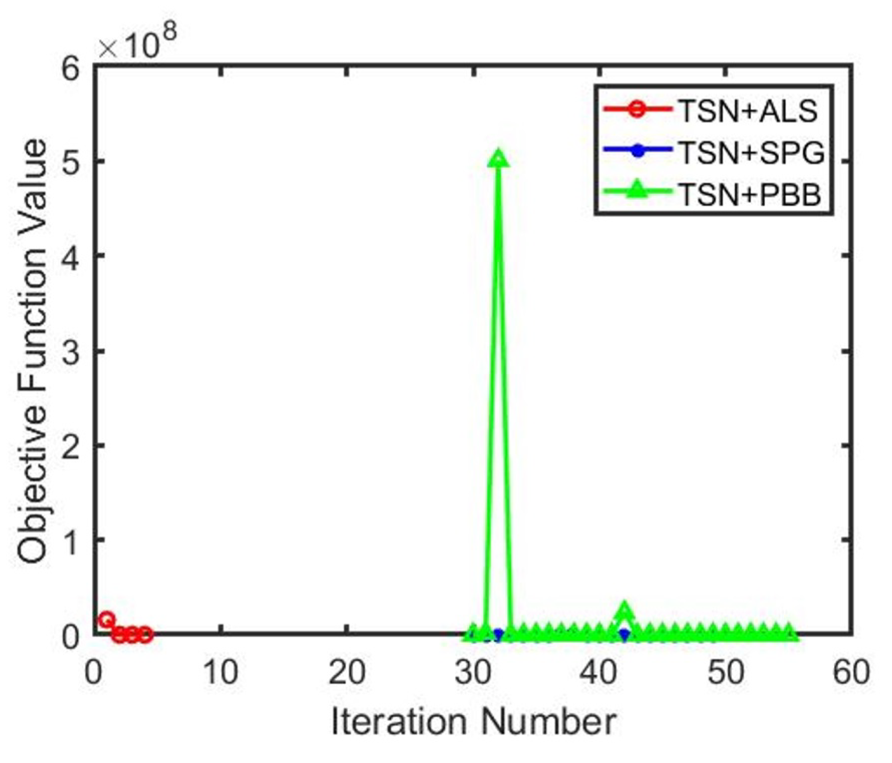
| Methods | Features(dim*nSample) | Parameters | Times(s) | Iter. | Error | Relative Error | Obj-Val |
|---|---|---|---|---|---|---|---|
| ALS | TSN (2048*660) | 0.4880 | 4 | 0.5972 | 2.0137 | ||
| SPG | TSN (2048*660) | 6.1992 | 49 | 0.4706 | 32.0130 | ||
| PBB | TSN (2048*660) | 23.5855 | 56 | 0.6146 | 10.0185 |
Disclaimer/Publisher’s Note: The statements, opinions and data contained in all publications are solely those of the individual author(s) and contributor(s) and not of MDPI and/or the editor(s). MDPI and/or the editor(s) disclaim responsibility for any injury to people or property resulting from any ideas, methods, instructions or products referred to in the content. |
© 2023 by the authors. Licensee MDPI, Basel, Switzerland. This article is an open access article distributed under the terms and conditions of the Creative Commons Attribution (CC BY) license (http://creativecommons.org/licenses/by/4.0/).

