
Submitted:
30 May 2023
Posted:
30 May 2023
You are already at the latest version
Abstract
Visual inertial SLAM algorithms enable robots to autonomously explore and navigate in unknown scenes. However, most of the current SLAM systems highly rely on static environment assumptions, which fails in the exsitence of motional objects in the real environment. To improve the robustness and localization accuracy of SLAM systems in dynamic scenes, this paper proposes a visual-inertial SLAM framework that fuses semantic and geometric information, called DA-VINS. First, this paper presents a dynamic object classification method based on feature’s current motion state, which obtains temporary static features in the environment. Secondly, a features dynamics check module based on IMU prior and adjacent frame’s geometry constraint is designed to calculate dynamic factors. It also verifies the classification results of temporary static features. Finally, a dynamic adaptive bundle adjustment module based on the features’ dynamic factors is designed to adjust the weights of features in nonlinear optimization. We evaluated our method in public and our dataset. The results show that D-VINS is one of the most real-time, accurate, and robust systems in dynamic scenes.
Keywords:
VISLAM
; dynamic environments
; object detection
; geometric constraint
; IMU prior constraint
1. Introduction
Simultaneous localization and mapping (SLAM)[1] is the crucial technology for advanced robotics applications, such as collision-free navigation and environment exploration[2]. It relies on the sensors carried by robots to accomplish high-precision localization and environment mapping simultaneously. Visual SLAM (VSLAM) [3,4] estimates the robot’s location by cameras, which has advantages of inexpensive, less energy-consuming and less computationally demanding. Visual-Inertial SLAM (VISLAM) [4] integrates IMU with camera to further improve the positioning accuracy and robustness of VSLAM system. Over the last decade, VSLAM framework has developed rapidly, with great open-source frameworks such as MSCKF[6], VINS-Mono[7], ORB-SLAM3[8], DM-VIO[9]. These open-source SLAM algorithms are classified into two categories according to different optimization methods: filter-based methods and nonlinear optimization-based methods. The filter-based approach uses Kalman filter with extended algorithms to estimate the robot’s state. The advantages of filter-based methods are that they can be deployed on embedded platforms. For example [10] is the visual-Inertial odometry(VIO) that integrates camera and IMU by ESKF. Optimization-based SLAM utilizes nonlinear optimization in the back end, such as Gaussian Newton, Levenberg-Marquardt, DogLeg. Nonlinear optimization provides higher accuracy but higher computational consumption. [11]is a VISLAM system that utilizes optical flow to track feature points at the front-end and optimizes the minimum reprojection error to solving the poses with bundle adjustment(BA) at the back-end; ORB-SLAM2[12] uses ORB feature points to improve tracking and adds a loop closure thread to obtain higher accuracy global pose. Based on ORBSLAM2, ORB-SLAM3 adds IMU to enhance the robustness of the system and is one of the best VISLAM so far. Those open-source frameworks have high accuracy and robustness in static environments. However, in the real world, all of the mentioned algorithms lose accuracy or even fail in localization with numerous dynamic objects in city streets or rural roads.
As early as 2003[13], there have been some studies on SLAM in Dynamic Environments (SLAMIDE) problem. The key to the dynamic SLAM problem is to detect dynamic objects in the environment.We classify dynamic SLAM methods into two categories: geometric-based methods and semantic-based methods. Geometry-based methods utilize constraints provided by camera movement between frames. But they ignore the potential motility of objects leading to missed detection of moving object. Semantic information-based methods can accurately identify potential moving objects through deep learning. However, large networks are hard to deploy in embedded platforms. The real motion state at current frame is also unknown.
To address these issues, we extends the work of VINS-Fusion and proposes a robust dynamic VISLAM, called D-VINS. D-VINS integrates semantic information and geometric constraints to divide features into different classes and adjusts the features’ weights in cost function accroding to different feature dynamics class. The main contributions of this paper are summarized as follows:
- A feature classification using YOLOV5 [14] object detection algorithm is proposed in the front-end, which divide dynamic feature points into three categories: absolute static points, absolute dynamic points and temporary static points. Then, dynamic factors of temporary static features are calculated based on the IMU pre-integration prior constraint and the epipolar constraint. Temporary static features are classified again according to dynamic factors.
- A robust BA optimization method based on dynamics factor is proposed in the back-end. If the object is more dynamic, its features weights are decreased, and vice versa, its features weights are increased.
- Extensive experiments are carried out on public datasets like TUM,KITTI and VIODE and our dataset. The experiment results demonstrate the accuracy and robustness of our proposed D-VINS.
2. Related Work
Most SLAM systems suffer severe accuracy loss in dynamic scenes. In terms of methods, Dynamic SLAM can be divided into two categories, geometry-based methods and semantic-based methods.
2.1. Geometry Based Dynamic SLAM
The geometry-based method utilizes geometric constraints between camera frames to remove outliers. Dynamic objects can be selected out because they are not conform the geometric motion consistency between frames. In addition, the inner points(static points) can be separated from the outliers(dynamic points) by statistics. The majority SLAM systems employs RANSAC[15] with epipolar constraints to remove outliers, such as VINS-Mono. It calculate the fundamental matrix by the eight-point method RANSAC. However, RANSAC is not work when the outliers are dominant. DGS-SLAM [16]proposes a RGB-D SLAM in the dynamic enviroment, which decomposes the camera motion into two parts, translation and rotation. Two geometric constraints are proposed to localize dynamic object regions. Besides, the method reduces the impacts of outliers in optimization by designing new robust kernel functions. DynaVINS[17] proposed method without deep learning to identify the dynamic features, which designs a novel loss function with IMU pre-integration results as prior in the bundle adjustment. In loop closure detection moudule, the loops from different features are grouped for selective optimization. PFD-SLAM [18]utilizes GMS (Grid-based Motion Statistics)[19] algorithm to guarantee the matching accuracy with RANSAC. Then it calculates homography transformation to extract the dynamic region, which is accurately obtained with particle filtering. ClusterSLAM[20] clusters feature points according motion consistency to reject dynamic objects. In general, geometry-based methods have higher accuracy and less computational cost than deep learning-based methods. But they lacks semantic information for precise segmentation. Meanwhile, geometry-based methods heavily rely on experience-based hyperparameters, which will significantly reduce algorithm feasibility.
2.2. Deep Learning Based Dynamic SLAM
At present, deep learning networks in object detection, semantic segmentation, optical flow, have made continuous breakthroughs in speed and accuracy. They can obtain the object detection results, like bounding boxes for SLAM systems in dynamic environments. In order to obtain the real motion state at the current frame, geometric information are usually added in deep learning based methods for accurate dynamic object recognition and rejection.
For example, DynaSLAM[21] is the first known dynamic SLAM sysetm that combines multi-view geometry and deep learning. It uses MASK R-CNN that provides pixel-level semantic priors for potential dynamic objects in images. Dynamic-SLAM[22] detects dynamic objects by SSD (Single Shot MultiBox Detector)[23] object detection network and compensates the missing detection problem based on constant velocity motion model. They set a threshold for average parallax of features in bounding boxes area to further reject dynamic features. However, this method relies on bounding boxes, which may causes wrong rejection of static feature points belonging to the background. DS-SLAM[24] utilizes SegNet network to eliminates dynamic objects’ features, which are tracked with Lucas–Kanade (LK) optical flow[25]. For matched points, fundamental matrix is found with RANSAC with the most inliers. The distance from the matched points to their epipolar line is obtained. If the distance is higher than a certain threshold, the point is regarded as a dynamic point and will be deleted. In addition, depth information provided by the RGB-D camera is usually used for dynamic object detection. Dynamic-VINS [26] proposes RGB-D based visual inertial odometry for embedded platforms, which reduces computational burden using grid-based feature detection algorithms.The dynamic features’ semantic label and depth are combined to separate the foreground and background. Moving consistency check based on IMU pre-integration is proposed for missed detection problem. YOLO-SLAM[27] is a RGB-D SLAM system that obtains object’s semantic labels by Darknet19-YOLOv3. SG-SLAM[28] is a real-time RGB-D SLAM system which adds dynamic object detection thread and semantic mapping thread based on ORB-SLAM2 for creating global static 3D reconstruction maps.
Generally, the advantage of geometry-based methods is fast. But they lack semantic information and cannot detect moving targets using prior knowledge of the scene and robustness are usually lower than deep learning based methods. Deep learning based methods have advantages in dynamic object detection. They can segment potential dynamic objects with semantic information. But deep learning is hard to run in real-time on embedded platforms and its accuracy is highly dependent on the results of training. In addition, most of the above methods uses RGB-D cameras,where geometric information is tightly-coupled with depth information.Those methods are more reliable in indoor environments. There are few algorithms that are suitable for outdoor dynamic scenes. We propose a dynamic SLAM that combines geometric information and semantic information. IMU prior constraints are tightly-coupled in dynamic features check and optimization. We fused those model into VINS-Fusion to attain better performances in both indoor and outdoor dynamic scenes.
3. Methods
The system is implemented based on VINS-Fusion, which is divided into three sections: data preprocess, features detection and tracking, bundle adjustment optimization. Figure 1 shows the illustration of system workflow.
Firstly, the color image are sent to the YOLOV5 to obtain semantic labels of the COCO dataset[29] and the bounding boxes of objects. In dynamic object classification, bayesian updating is employed to distinguish absolute dynamic objects, absolute static objects and temporary static objects. The harries keypoints are extracted and only those points from absolute static objects and temporary static objects will be tracked by LK optical flow in the front end. The IMU sensor provides features states, like translation, rotation and velocity with prior motion constraints. The feature’s dynamic factor is the root mean square of IMU pre-integration error and epipolar constraint. In feature dynamics check, the dynamic factors of temporary static points are calculated, whose numerical value indicates the movement of feature points. A larger numerical value shows indicates that the feature points are likely to be dynamic.The key of feature rejection strategy is to preserve potential points judged by dynamic factors, instead of removing all the movable points. This strategy increases the number of feature points in the high dynamic scene to guarantee the sufficient features for localization.
At the back-end, we proposes a novel loss function with adaptive weights based on dynamic factors in BA adjustment. Feature weights are added into cost function as parameters to be optimized. D-VINS divides conventional optimization process into two steps. Firstly, features’ weights are fixed the to optimizes system states separately. Then system states are fixed to optimize the weights. The above process is iterated until required times or weights are converged. In addition, dynamics factors are added to adjust features’ weights.
3.1. Dynamic Object Classification
Tracking static features is the key for SLAM systems to maintain localization accuracy in dynamic environments. However, in most scenes, dynamic objects are movabel instead moving, which is the drawback of pure deep learning based methods. The boundary between dynamic and static objects is not clear for deep learning. For instance, books are commonly considered as static objects. But when a person holding a book, the book becomes a dynamic object, which is the same as a car in a parking lot or running in the highway. Therefore, semantic information is not enough to assist robots to detect the moving objects in dynamic environment. In D-VINS, we propose a classification method for obtained semantic labels.
3.1.1. Semantic Label Incremental Updating with Bayes’ Rule
In order to recognize most objects in life, we selected COCO dataset to training the YOLOV5, which contains 80 categories of common objects. Not all objects need to be detected. So we selected 17 most common categories. Firstly, color images are input to the YOLOV5 with TensorRT [30] accelerating to obtain semantic labels of COCO categories. Bounding boxes can locate the approximate region of a dynamic object in an image. The feature points inside the bounding boxes will be given its semantic labels. Since object detection network can only detect semantic information of the current frame and exists missing or incorrect detection problem,D-VINS updates features’ semantic label according to Bayes’ rule to to avoid the error in a certain frame, which transforms the labeling problem into a maximum a posteriori problem.
The th map point in a given world coordinates is observed byth frame can be written as . denotes the pixels in camera coordinates that corresponds to the th map point. The projection process of feature points is as follows:
Where,is the depth of map points and is the extrinsic matrix. denotes the transformation matrix from the world coordinates to the observation frame. Denote and as the ground truth of the semantic labels of the th feature points from the beginning frame to the th frame and the measurements of deep learning bounding boxes. According to Bayes’ rule, there is:
In fact, this is a Maximize a Posterior problem, shown as:
When dynamic objects are detected in previous frames, the same result should also be obtained by the current frame. So the semantic labels of feature points are affected by multi-frame in the past. The semantic label probability distribution of theth feature point inth frame is:
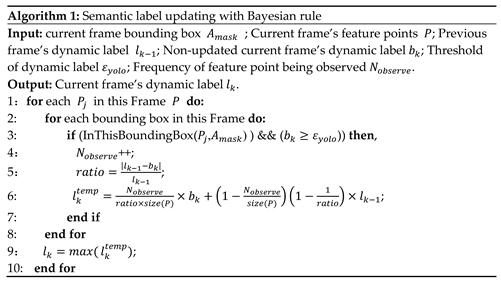
When the semantic information of the current frame is obtained, D-VINS will determine whether it is consistent with the previous frames. If the previous semantic label is same as that in the current frame, the detection resut of the current frame is more trusted, and vice versa. The specific algorithm steps are shown in Algorithm 1.
3.1.2. Feature Points Motion State Classification
The feature points classification is divided into two parts. The first part is to classify COCO categories according to the possibility of motion based on life experience. The classification is divided into 1~5 levels. the higher the level the higher the possibility of movement. Those five levels are level I public facilities (traffic light, bench), Level II furniture (chair, sofa, bed), Level III transportation (bicycle, car, motorbike, bus, truck, boat), Level IV sports (football, basketball), people (person) and Level V animals (cat, dog, bird), seen in the Figure 2.
The second part is to classify the feature points into three categories according to the movement in their current frame, which can be divided into absolute stationary points, temporary stationary points and absolute dynamic points. In general, if one object is detected as bench, sofa or potted plant, its feature points are most likely to be a static, which can be involved in the pose estimation and mapping. If the semantic label is animal such as birds, cats or dogs, those features are considered to be dynamic features. Animals usually keep moving and occupy a small area in an image, which have less impact on the SLAM system. As shown in Figure 2, objects of level I and level II are considered as absolute static objects, objects of level III and level IV are temporary static objects and objects of level V are absolute dynamic objects. For temporary static objects, their motion state cannot be determined by prior semantics from deep learning. If such feature points occupy a large area in the image, eliminating all of them will impair the localization accuracy due to insufficient feature points for tracking.
3.2. Features Dynamics Check with IMU Prior and Epipolar Constraint
In order to check current motion state of movable objects, D-VINS calculate dynamic factors to find the absolute dynamic points. For absolute static objects, like furniture, traffic lights and benches, their feature points are kept for all process of SLAM system. For absolute dynamic points like animals, all those feature points are removed and do not participate BA optimization or global pose optimization. For temporary static points, the first part of dynamic factors is calculated by IMU pre-integration, which is utilized as the initial pose of current frame to obtain the reprojection error by projecting the 3D feature points onto the image plane. According to eipipolar geometry, the foundational matrix is calculated to obtain the distance from feature points to their epipolar lines, which is the second part of dynamic factor. If one of the dynamic factors of the feature point is lower than a certain threshold, the point will be labeled as absolute dynamic points.
3.2.1. Dynamic Factor of Reprojection Error Based on IMU Prior Constraint
Conventional visual reprojection projects a feature point from its previous observed frame to the pixels plane of current frame. The reprojection error cannot be calculated if camera pose of current frame is unknown. IMU preintegration provides an initial estimate for current frame’s camera pose, which enables calculating reprojection error to reject dynamic objects with the IMU sensor.
There must be errors between the estimation pose and real camera pose, which means the reprojection points and the observation points are usually not coincident. For map point in world coordinate , its pixel coordinates projected on the jt frame is . According to Equation (1), the relationship between map points and pixel points according to the camera projection model exists as follows:
Equation (5) can be written in matrix form and the resisual of the reprojection error as follows:
is the Lie algebra of the th frame in body frame and is the intrinsic matrix obtained by camera calibration[31]. The camera pose ofth frame is obtained by IMU preintegration:
where, , and are the pre-integration terms of position, velocity, and pose, which changes the reference frame from the world frame to the local body frame; , and are system state the state of the jth body frame. From equation (7), the pose of jth frame is obtained. The pixel coordinates in jth frame projected from ith frame is . And the observation in jth frame is . By equation (6), the new visual reprojection resisualof map point can be established by camera projection model:
where, is the transformation matrix from the body frame to camera frame, which is obtained by Kalibr[32]. and represents the transformation matrix between imu frames and the world coordinate. and are translation matrix between body frame and world frame. represents the inverse depth of feature point P.represents the pinhole camera projection model.
As shown in the Figure 3, the distance in red denotes the dynamic factor of IMU reprojection error,which is utilized to evaluate how far the object is away from the main optical axis. It shows the observation and projection of the static map point P and the dynamic point P’ in two camera frames. O denotes camera’s optical center. and are feature points matched for the two frames with optical flow. is the feature point projected by the static point P in jth camera frame. is the feature point projected by the dynamic point P’ in j-1th camera frame.
Generally, it is effective to determining the dynamics of the object by feature points reprojection error. However, this method will fail when the dynamic object is moving along the camera’s optical center ( either toward or away from the camera), which is shown in Figure 3. The reprojection error is close to 0 even P is not a dynamic point. Therefore, we propose additional reprojection error on the previous frame to the conventional visual reprojection in equation (8). Even the point is moving along the optical center, there will be at least one reprojection error is not close to 0. So the two reprojection process are complementary to each other, which minimizes the effect on the dynamic judgment of feature points with the special object motion direction. Then the first part of the dynamic factors is obtain as below:
3.2.1. Dynamic Factor of Epipolar Constraint
Epipolar constraint is a critical property to limit the position of feature points, which is frequently utilized to accelerate the matching process at the front end in various SLAM systems. In D-VINS, the data association between the feature points is obtained by pyramidal iterative Lucas-Kanade optical flow. Then, the seven-point method based on RANSAC is used to calculate the fundamental matrix between two camera frames. The epipolar lines of feature points in the current frame are calculated with the fundamental matrix. The distance from a point to its epipolar line is defined as the second part of dynamic factor. Finally, the distance is used to determine whether the point is dynamic or not. According to the pinhole camera model, the map point P is observed by different camera frames, which is shown in Figure 4. x1 and x3 are matched feature points in different frames, and x2 is the feature point projected to the jth frame by the map point P. The short dashed lines I and I’ are the epipolar lines of the two frames.
are the homogeneous coordinate forms of the two matched feature points, belonging to the j-1th frame and jth frame, respectively. Then, the epipolar line of in the jth frame is as follows:
Where ,anddenote the real constants in general form of a straight line(Xu+Yv+Z = 0). F denotes the fundamental matrix. Then, for feature point , the epipolar constraint is as follows:
In Figure 4, the distance from the point to the epipolar line is marked by the blue line. For the matched feature point of , the residual of epipolar constraint can be described as follows:
Then the second part of the dynamic factor is obtain as below:
For the features of static objects, should be 0 or close to 0. But for the features of dynamic objects, like P’, there is an offset between the real pixel coordinates and its observatoin. But when the feature point moves toward the optical center of j-1 frame, the feature point is still on its epipolar line. So it is hard to determine whether the object is in motion or not. Therefore, when defining whether features are in moving state, it needs to combine the two distances of and.
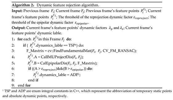
The threshold of the reprojection dynamic factor is set to 4 pixels and of the epipolar dynamic factor is set to 3 pixels. If the errors exceeds those thresholds then the feature points are considered as absolute dynamic points and rejected. Then the feature is marked as ADP. So far, the two dynamic factors and are obtained.
This method enables a more accurate classification of temporary static objects and finds the dynamic feature points. In addition, the feature points of dynamic objects with small movements can be fully utilized by the SLAM system. The specific algorithm steps are shown in Algorithm 2.
3.3. Dynamic Adaptive Bundle Adjustment
The current conventional bundle adustment optimization maintains the same weight for all feature points, and is not effective to reject outlier and dynamic points. Meanwhile, higher weights should be set for absolute static features and the weights for dynamic points should be reduced to ensure localization accuracy. For dynamic points with lower dynamics, the weights of their feature points should be positive correlation to the dynamic factor. Therefore, in addition to distinguishing dynamic and static objects by empirical thresholds in subsection 3.2, this study designs a novel bundle adjustment optimization algorithm based on the dynamics factor.
3.3.1. Conventional Bundle Adjustment Optimization
In the conventional visual-inertial state estimator, the bundle adjustment optimization equation is as follows:
where, denotes the huber kernel function. represents marginalization residuals, represents IMU pre-integration residuals and represents visual reprojection error. represents the marginalization of the measurement state estimation matrix, represents IMU observation and represents visual observation. denotes the covariance of IMU measurement and denotes the visual covariance. represents the set of all IMU observations, represents the set of tracked features in sliding window and denotes the estimated states to be optimized.
It shows that the traditional bundle adjustment formulation can neither reject nor change the weights of the dynamic feature points. If all temporary static points are eliminated, the visual observations for optimization will be insufficient. This leads to unstable or error BA optimization result, so a more robust BA optimization approach needs to be implemented.
3.3.2. Dynamic Adaptive Cost Function with Dynamic Factors
This noval cost function has two features. The first is to reject dynamic features, while the second is to adjust the weights of feature points in optimization according to the dynamics factors. Inspired by DynaVINS,we proposes the form of dynamics-adaption loss function as follows:
Where, and denotes two dynamic factors of a feature point in frame j. denotes the weights of feature points and the weight is fixed to 1 with absolute static points. represents dynamic lable, which will be 1 with absolute static points and 0 with temporary static points. Equation (17) denotes the dynamic factors. For absolute static points, the is 1 and the back-end optimization loss function is the same as the conventional one. For temporary static points, the loss function will switches to shown in equation (16). As the loss function is designed in a non-linear quadratic form, the optimal weights can be derived as follows:
After optimizing the weights, those features with higher dynamic factor will be lower weights. The losses’gradient of those features will be close to zero, which have no impact on BA. Quadratic form is designed for non-linear form because linear system doesn’t need optimization. is a constant parameter used to increasing gradient value and convexity, which is set to 2 empirically. Different from DynaVINS, the weight momentum factor doesn’t need with the help of semantic labels and the points weights are delivered with bounding boxes. is utilized instead of the pure huber kernel function in the conventional cost function. The total cost function based on the dynamic factors is as follows:
This algorithm aims to utilize as many feature points as possible, as well as to maintain the accuracy of pose estimation. The strategy is to increase the weight of absolute static points and decrease the weight of temporary static points in BA optimization, completely discarding absolute dynamic points in optimization. In addition, the threshold is a hyperparameter, which requires specific adjustment according to the environment and equipment.It makes the algorithm difficult to be widely used. To improve the algorithm applicability, a loose threshold is set in this paper to fit the majority scenes.
In order to avoid artificial adjustment of hyperparameters that lead to the degradation of the applicability of the system, the weights of feature points are optimized to obtain more robust localization results. In optimizing the current state , the weights of each feature point are fixed. After that, the current state is fixed, and feature points weights are optimized according to the dynamic adaptive cost function,which is as follows:
Since the feature points weights are independant from each other the overall loss function is obtained by accumulating the cost equations of each feature point:
Ultimately, different optimization weights can be used based on different dynamic factors of the feature points.
4. Experimental Results
In this section, the effectiveness of D-VINS is validated. Public dataset, like TUM RGB-D[33], KITTI[34] and VIODE[35] are utilized to verify the performance of the algorithm in different dynamic scenes. The experimental results will be analyzed from qualitative and quantitative perspectives. The results include the comparison of DVINS with the original algorithm (ORB-SLAM2, VINS) and the state-of-the-art dynamic VISLAM algorithm (DynaVINS). We integrated D-VINS with ROS and all experiments were run on a laptop with 16GB RAM (CPU: AMD Ryzen7 5800H, GPU: NVIDIA GEFORCE RTX 3050TI).
In this paper, the root mean square error(RMSE) of absolute trajectory error (ATE) and the root mean square value of relative positional error (RPE) are selected as evaluation metrics. The unit of ATE is m. The unit of translational drift in RPE is m/s, and the unit of rotational drift is °/s.They represent the global consistency of the trajectory and the drift of the odometer per unit time, respectively.
4.1. TUM RGB-D, VIODE and KITTI Dataset Evaluation
4.1.1. TUM RGB-D Dataset
The TUM RGB-D dataset was obtained by a Microsoft Kinect camera at a 30Hz frame rate and contains 39 image sequences containing both color and depth images. it has become one of the most commonly used datasets for evaluating visual odometry in dynamic scenes, and numerous algorithms, such as DS-SLAM and SG-SLAM, have validated their algorithms on this dataset. The ground truth of camera motion is acquired by a high precision motion capture system. The dataset provides 9 sequences for dynamic scenes, where dynamic objects move at different levels and can be divided into low and high dynamic sequences. The low-dynamic sequences are named by sitting (fr3/sitting_static, fr3/sitting_xyz, fr3/sitting_halfsphere, fr3/sitting_rpy), both sitting on a stool with less movement; High-dynamic sequences are named by walking (fr3/walking_static, fr3/walking_xyz, fr3/walking_halfsphere, fr3/walking_rpy). Two people will walk back and forth in front of the camera as high-dynamic objects, as well as sitting on a chair as low-dynamic objects. Since it contains dynamic objects like moving person, and usually occupy more than half of the image. It is reliable to verify the feasibility of SLAM algorithm in dynamic scenes. In addition, TUM dataset contains no IMU data and VINS does not support monocular VO mode, so modules contains IMU was excluded from D-VINS for experiment.
In this paper, we use the open source trajectory evaluation tool Evo (Available online: https://github.com/MichaelGrupp/evo (accessed on 25 April 2023)) to visualize the trajectory differences between D-VINS and ORB-SLAM2. And the ATE and RPE of each algorithms are analyzed with groud truth. The data were obtained from the actual experiments in the dataset.The Figure 5 shows the plotted trajectories of the two algorithms. The black dashed line represents the ground truth, provided by the dynamic capture. The blue solid line represents the trajectory generated by D-VINS and the green solid line represents the trajectory generated by ORB-SLAM2 for comparative analysis. According to figure (h), it can be seen that when dynamic objects appeared, it causes serious impairment to the trajectory accuracy. The quantitative analysis of this figure fully demonstrates the necessity of dynamic object rejection and the effectiveness of D-VINS.
Table 1 summarizes the quantitative experimental results of ORB-SLAM2 and D-VINS for TUM 7 sequences. The horizontal line in (h) represents loopback detection. According to the experimental results, D-VINS outperforms ORB-SLAM2 in six sets of experiments, which proves the effectiveness of its dynamic object identification and rejection method. Since the person sitting on the chair in "fr3_sitting_xyz" sequence remains stationary for a long time, the dynamic feature points occupy a lower percentage of the view. And this has little impact on the localization accuracy. Whereas in "fr3_walking_rpy" and "fr3_walking_static" sequences, due to the large movement of persons, the dynamic feature points occupy a larger portion of the view. This will severely impair the accuracy of visual localization. The D-VINS shows a good localization accuracy even though it is not a pure visual odometer. The reliability dynamic object recognition and rejection with deep learning and geometric constraints is verified with this dataset.
4.1.2. KITTI Dataset
The KITTI dataset provides sequences containing stereo color images in 00 to 10 urban street and highway environments for evaluating the accuracy of odometry localization. The table shows the results of one of the sequences 05 and 07 in comparison with VINS-Fusion and DynaVINS and the bolded data indicate the best performance, as shown in Figure 6. Since dynamic objects on both 00 and 05 sequence streets are sparse, dynamic object rejection provides limited improvement to the system accuracy. The experimental data are obtained from real measurements, rather than directly from the paper to compare the generalizability of the algorithms. As shown in Table 2, the localization accuracy and dynamic feature recognition rejection of DynaVINS are highly dependent on the hyperparameters (momentum factor and regularization factor). Therefore, its localization results in different data sets are worse and it is hard to keep the algorithm to localize with high accuracy even after a long time of parameter adjustment. Experimental results on the KITTI dataset show that D-VINS has better generalizability than DynaVINS,and has a certain accuracy improvement compared to VINS-Fusion.
4.1.3. VIODE Dataset
VIODE is a simulation dataset for testing VIO performance in dynamic environments such as urban areas, filling the gap in dynamic VIO system evaluation. The dataset simulates the UAV localization problem in different dynamic environments (daytime city street environment, dark city street environment and underground parking environment). Each scenes are divided into 4 sequences according to the number of dynamic objects. 0_none, 1_low, 2_mid and 3_high has a total of 12 sequences. In the high sequences, the camera field of view is included with the entire occlusion to evaluate the localization accuracy and system robustness of the VIO in extreme situations. The dataset contains time-synchronized stereo color images, IMU data, instance segmentation mask and ground truth of trajactory. To validate the accuracy of the algorithm for the dynamic recognition of absolute dynamic points and Temporary static points, D-VINS and DynaVINS are both compared. VINS-Fusion is also involved in the comparison to prove the necessity and effectiveness of the dynamic rejection module. The hyperparameters in DynaVINS use the same values as in the paper, regularization factor and momentum factor .
In general, the bundle adjustment of D-VINS incorporating the dynamics factor achieves the most accurate pose estimation results in static scenes as shown in Table 3. It has better localization accuracy in low dynamic scenes and has similar accuracy to DynaVINS in high dynamic scenes, even a better performance of D-VINS in some sequences. D-VINS removes feature points that are far away or negative in depth after BA. And with the help of RANSAC, there is a certain resistance to the influence of dynamic objects. But these features affect the results of BA before they are deleted and also damage the effectiveness of RANSAC as the number of dynamic objects in the field of view increases. Eventually the combined leads to an increase in the error of the D-VINS trajectory. In addition, the spacing and number of feature points in the front end can significantly affect the performance of D-VINS. Stereo system accuracy is seriously impaired when remote features occupy the majority of the field of view or the feature spacing is too small. So for the same parameters in the City sequence, VINS and D-VINS does not perform as well as in the parking_lot environment. The localization accuracy of DynaVINS relies highly on the hyperparameters, regularization factor and momentum factor. However, those hyperparameters rely on manual experience and are badly generalized to scenes. The same values have very high localization accuracy in some scenes, but are not suitable for other sequences. For instance, the localization accuracy of DynaVINS in the City_day dataset is not stable.
For dynamic scenes with low occlusion, D-VINS contains a deep learning module that can identify dynamic objects by observing their full appearance and calculate the dynamic factors, based on the geometric characteristics. D-VINS offers higher accuracy in dynamic feature point screening than DynaVINS, which rejects dynamic objects in a purely geometric manner,like(d), (h) and (l) in Figure 7. Therefore, the positioning accuracy is higher in low and mid sequences. The green feature points are Absolute static points, the white feature points are Absolute dynamic points, and the purple feature points are Temporary dynamic points. Due to the dynamic object is close to the camera, D-VINS fails with deep learing network to detect the object in the high occlusion environment. Currently, D-VINS relies heavily on dynamic factors and the accuracy of feature point segmentation is reduced, but it is still robust for this challenging environment, as 3_high sequence in City_day.
4.2. Data Collecting Equipment and Real Environment Dataset Experiments
To demonstrate D-VINS can be applied to real project, we builds a self-made data acquisition device and creates a dataset with it.
4.2.1. Data Collection Devices and Real Datasets
The device integrates GNSS, inertial navigation, LIDAR and stereo camera which is mainly divided into two parts, the handheld part and the backpack part. As shown in Figure 8, the device has three working modes, handheld, backpack, and vehicle working mode. The handheld part includes GNSS antenna, Velodyne VLP-32C mechanical LIDAR, Inertial Labs INS-D GNSS/IMU inertial guidance, ZED2 color binocular camera, and the backpack part includes NVIDIA Jetson AGX Xavier processor, 12V DC lithium battery, MD-649 4G DTU 4G communication module and antenna. In this paper, one handheld rural sequence and two city street sequence were selected for experimental validation:
- 5_SLAM_country_dynamic_loop_1 sequence was collected in a village in Xiangyin County, Yueyang City, Hunan Province, in a relatively open environment, where a pedestrian and child were always present in the image moving in synchronization with the camera. The start and end points of the sequence are close to each other, but there is no loop clouse to detect the drift.
- 14_SLAM_car_road_1 sequence is a street in Xiangyin County, Yueyang City, Hunan Province. The sequence is an open environment. This environment is challenging for stereo visual localization, which causes severe drift. Rural roads are narrow with many vehicles, and there are villager gatherings in the middle of the road. Pedestrians and vehicles are intricate and occupy a large field of view, making positioning difficult and challenging.
- 18_SLAM_car_road_2, sequence is an urban environment with wider roads, more vehicles and more pedestrians compared to 14 rural streets. It is suitable as a dynamic rejection algorithm evaluation sequence. The main data types include: GNSS raw data, IMU data, LiDAR point cloud data, and binocular color image data. The ground truth of trajectory is obtained with GNSS RTK.
4.2.2 Feature Classification Results in Real Dataset
In 5_SLAM_country_dynamic_loop_1 sequence, there are two person walking in front of the camera, which is easy for deep learning to accomplish object detection task. As shown in Figure 9, if the person with jacket is moving in the second row in (a), the dynamic features are segmented accurately. When the person is movable but remian static at current time shown in first row in (a), those feature points are kept for optimization. In high dynamic sequence, the majority of points are movable and only few of them is moving. D-VINS is able to reject dynamic features that close to the camera with higher dynamic factors. In the city street, the cars parked on the roadside and driving on the road are detected with different motion state classification.
4.2.3. Trajectories Results in Real Dataset
This paper compares the results of the current state-of-the-art algorithms DynaVINS and D-VINS, VINS algorithms in real data set sequences. D-VINS gets better measurement results in real data sets, effectively overcoming the influence of dynamic objects. As shown in Table 4, D-VINS obtains better localization accuracy than DynaVINS in the 5_SLAM_dynamic_loop_1 sequence. Even though the ATE RMSE is similar to VINS, more detailed results show that D-VINS has more accurate localization accuracy in the presence of dynamic objects, and D-VINS has a lower median and mean. Even after parameter adjustments, DynaVINS had difficulty finding parameters that could accomplish good accuracy in localization (those hyperparameters provided in the paper could not accomplish localization, even though they worked well in the VIODE and KITTI datasets). The high reliance on equipment and hyperparameters is also the drawback for geometry-based methods. In Figure 10, D-VINS achieves excellent positioning results in two road sequences without loop detection. The pure VIO system (no global optimization and loopback detection) can effectively reduce the influence of dynamic objects and substantially exceed the positioning accuracy of VINS. In summary, D-VINS has stronger robustness and scene applicability in dynamic scenes compared to other algorithms.
5. Discussion
In the experimental results of Table 1, Table 2, Table 3 and Table 4, D-VINS and these contrasting SLAM systems all finished the validation experiments. In terms of the ATE and RPE, D-VINS achieved better performance in 6 sequences in TUM RGB-D dataset. ORB-SLAM2 can’t identify static and dynamic features and only achieves quite accurate results for low dynamic sequences. In the high dynamic sequences, the performance of ORB-SLAM2 is significantly reduced. Table 1 validates the effectiveness of the dynamic rejection with deep learning and epipolar constraints in D-VINS, which is not a pure VSLAM, but still achieve good localization accuracy. Table 2 displays the results in KITTI sequences, which demonstrate the effectiveness of D-VINS in outdoor scenes. The state-of-the-art DynaVINS can segment features without prior semantic information and reached high accuracy in VIODE simulation dataset, shown in Table 3. But DynaVINS is highly relied on the two hyperparameters, which is difficult to achieve the same high accuracy in different datasets. In KITTI 05 and 07 sequences, dynamic objects is fewer than those in VIODE, which have less impact on position estimation. DynaVINS didn’t show great performance in the KITTI sequences, as it did in VIODE, displayed in Figure 6. For the highly occluded scenes appearing in VIODE dataset, deep learning will fail and the objects will move towards the camera optical center, shown in the first image of Figure 7b. D-VINS shows good dynamic features segmentation performance and trajectory accuracy,which shows D-VINS has better robustness in multiple environments shown in Figure 7b,d,f. However, the accuracy of DynaVINS decreases in dynamic objects with fewer sequences such as 0_none sequences.
In addition, D-VINS shows great perfomance in features classification and trajectory accuracy in the rural and city sequence, as shown in Figure 9. For our real datasets, DynaVINS is more difficult to accomplish localization task. Because the higher reprojection errors may come from the movement of the camera itself or from the dynamic features, weights just indicate the magnitude of the reprojection error instead of feature’s motion state. As both rural road and city road sequence are in large space without loop closure, VINS-Fusion shows worse performance compared to D-VINS.
It can be concluded from the above experimental results: D-VINS first classifies feature points twice with semantic information and IMU motion constraints, which is different from other dynamic SLAM methods. The hyperparameters of D-VINS are few and have good applicability to indoor-outdoor datasets, simulation datasets and our real scene datasets. The discussion shows that D-VINS has practical application potentiality aiming at dynamic scenes.
6. Conclusions
In this paper, we propose a new dynamic VIO system for outdoor dynamic scenes, which can significantly reduce the effect of dynamic objects. In D-VINS, it contains four modules: target identification and data pre-processing, feature point classification and tracking, back-end dynamic factor BA optimization. Dynamic object recognition relies on YOLOV5 to get semantic information about the scene, such as walking people and stopped cars. The semantic labels are incrementally updated, which divided dynamic points into absolute dynamic points, absolute static points and temporary static points. After that, the dynamic factors of temporary static points is calculated with IMU pre-integration and epipolar constraint. Only absolute static points and temporary static points are sent to nonlinear optimization. The feature point weights are adjusted according to the dynamic lable and dynamic factors in BA. The effectiveness of the system for dynamic environments is verified in the TUM RGB-D , KITTI , VIODE datasets and our dataset. The experimental results shows better performance than VINS and state-of-the-art method DynaVINS. However there are still many work to do in the future. For instance, to further expand the robotics applications, octree global maps have to be rebuilt. And the more effective loss function needs to be studyed. The problem of areas occluded by dynamic objects must be reconstructed with the help of multi-view geometry or deep learning methods to accomplish advanced robotic applications.
Author Contributions
Y.S. conceived the idea and methods; Data curation, Y.S., R.T., C.Y. ;Software, Y.S. ;Y.S., X.S.performed experiments and validation; C.Y., R.T. analyzed the data; Supervision, Q.W. and Y.F.; Y.S., C.Y.,R.T. and S.J. wrote and revised the paper. Visualization X.W. All authors have read and agreed to the published version of the manuscript.
Funding
This research was funded by National Natural Science Foundation of China (No.42074039). The authors would like to thank the referees for their constructive comments.
Data Availability Statement
Publicly available datasets were analyzed in this study. This data can be found here: http://vision.in.tum.de/data/datasets/rgbd-dataset, https://github.com/kminoda/VIODE, https://www.cvlibs.net/datasets/kitti/, which were all accessible on 1st May 2023.
Acknowledgments
We thank the researchers who for making TUM RGB-D, KITTI and VIODE datasets.
Conflicts of Interest
The authors declare no conflict of interest.
References
- Abaspur Kazerouni, I.; Fitzgerald, L.; Dooly, G.; Toal, D. A Survey of State-of-the-Art on Visual SLAM. Expert Systems with Applications 2022, 205, 117734. [CrossRef]
- Covolan, J.P.M.; Sementille, A.C.; Sanches, S.R.R. A Mapping of Visual SLAM Algorithms and Their Applications in Augmented Reality. In Proceedings of the 2020 22nd Symposium on Virtual and Augmented Reality (SVR); November 2020; pp. 20–29.
- Tourani, A.; Bavle, H.; Sanchez-Lopez, J.L.; Voos, H. Visual SLAM: What Are the Current Trends and What to Expect? Sensors 2022, 22, 9297. [CrossRef]
- Tourani, A.; Bavle, H.; Sanchez-Lopez, J.L.; Voos, H. Visual SLAM: What Are the Current Trends and What to Expect? Sensors 2022, 22, 9297. [CrossRef]
- Chen, C.; Zhu, H.; Li, M.; You, S. A Review of Visual-Inertial Simultaneous Localization and Mapping from Filtering-Based and Optimization-Based Perspectives. Robotics 2018, 7, 45. [CrossRef]
- Mourikis, A.I.; Roumeliotis, S.I. A Multi-State Constraint Kalman Filter for Vision-Aided Inertial Navigation. In Proceedings of the Proceedings 2007 IEEE International Conference on Robotics and Automation; IEEE: Rome, Italy, April 2007; pp. 3565–3572.
- Qin, T.; Li, P.; Shen, S. VINS-Mono: A Robust and Versatile Monocular Visual-Inertial State Estimator. IEEE Trans. Robot. 2018, 34, 1004–1020. [CrossRef]
- Campos, C.; Elvira, R.; Rodríguez, J.J.G.; M. Montiel, J.M.; D. Tardós, J. ORB-SLAM3: An Accurate Open-Source Library for Visual, Visual–Inertial, and Multimap SLAM. IEEE Transactions on Robotics 2021, 37, 1874–1890. [CrossRef]
- von Stumberg, L.; Cremers, D. DM-VIO: Delayed Marginalization Visual-Inertial Odometry. IEEE Robot. Autom. Lett. 2022, 7, 1408–1415. [CrossRef]
- Sun, K.; Mohta, K.; Pfrommer, B.; Watterson, M.; Liu, S.; Mulgaonkar, Y.; Taylor, C.J.; Kumar, V. Robust Stereo Visual Inertial Odometry for Fast Autonomous Flight. IEEE Robotics and Automation Letters 2018, 3, 965–972. [CrossRef]
- Qin, T.; Cao, S.; Pan, J.; Shen, S. A General Optimization-Based Framework for Global Pose Estimation with Multiple Sensors 2019.
- Mur-Artal, R.; Tardós, J.D. ORB-SLAM2: An Open-Source SLAM System for Monocular, Stereo, and RGB-D Cameras. IEEE Transactions on Robotics 2017, 33, 1255–1262. [CrossRef]
- Wang, C.-C.; Thorpe, C.; Thrun, S. Online Simultaneous Localization and Mapping with Detection and Tracking of Moving Objects: Theory and Results from a Ground Vehicle in Crowded Urban Areas. In Proceedings of the 2003 IEEE International Conference on Robotics and Automation (Cat. No.03CH37422); September 2003; Vol. 1, pp. 842–849 vol.1.
- Jocher, G.; Chaurasia, A.; Stoken, A.; Borovec, J.; NanoCode012; Kwon, Y.; Michael, K.; TaoXie; Fang, J.; imyhxy; et al. Ultralytics/Yolov5: V7.0 - YOLOv5 SOTA Realtime Instance Segmentation 2022. [CrossRef]
- Fischler, M.A.; Bolles, R.C. Random Sample Consensus: A Paradigm for Model Fitting with Applications to Image Analysis and Automated Cartography. In Readings in Computer Vision; Elsevier: Amsterdam, The Netherlands, 1987; pp. 726–740.
- Yan, L.; Hu, X.; Zhao, L.; Chen, Y.; Wei, P.; Xie, H. DGS-SLAM: A Fast and Robust RGBD SLAM in Dynamic Environments Combined by Geometric and Semantic Information. Remote Sens. 2022, 14, 795. [CrossRef]
- Song, S.; Lim, H.; Lee, A.J.; Myung, H. DynaVINS: A Visual-Inertial SLAM for Dynamic Environments. IEEE Robot. Autom. Lett. 2022. [CrossRef]
- Zhang, C.; Zhang, R.; Jin, S.; Yi, X. PFD-SLAM: A New RGB-D SLAM for Dynamic Indoor Environments Based on Non-Prior Semantic Segmentation. Remote Sens. 2022, 14, 2445. [CrossRef]
- Bian, J.; Lin, W.-Y.; Matsushita, Y.; Yeung, S.-K.; Nguyen, T.-D.; Cheng, M.-M. GMS: Grid-Based Motion Statistics for Fast, Ultra-Robust Feature Correspondence. In Proceedings of the 2017 IEEE Conference on Computer Vision and Pattern Recognition (CVPR); July 2017; pp. 2828–2837.
- Huang, J.; Yang, S.; Zhao, Z.; Lai, Y.-K.; Hu, S. ClusterSLAM: A SLAM Backend for Simultaneous Rigid Body Clustering and Motion Estimation. In Proceedings of the 2019 IEEE/CVF International Conference on Computer Vision (ICCV); October 2019; pp. 5874–5883.
- Bescos, B.; Fácil, J.M.; Civera, J.; Neira, J. DynaSLAM: Tracking, Mapping and Inpainting in Dynamic Scenes. IEEE Robot. Autom. Lett. 2018, 3, 4076–4083. [CrossRef]
- Xiao, L.; Wang, J.; Qiu, X.; Rong, Z.; Zou, X. Dynamic-SLAM: Semantic Monocular Visual Localization and Mapping Based on Deep Learning in Dynamic Environment. Robotics and Autonomous Systems 2019, 117, 1–16. [CrossRef]
- Liu, W.; Anguelov, D.; Erhan, D.; Szegedy, C.; Reed, S.; Fu, C.-Y.; Berg, A.C. SSD: Single Shot MultiBox Detector. In Proceedings of the Computer Vision – ECCV 2016; Leibe, B., Matas, J., Sebe, N., Welling, M., Eds.; Springer International Publishing: Cham, 2016; pp. 21–37.
- Yu, C.; Liu, Z.; Liu, X.; Xie, F.; Yang, Y.; Wei, Q.; Fei, Q. DS-SLAM: A Semantic Visual SLAM towards Dynamic Environments. 2018. [CrossRef]
- Lucas, B.D.; Kanade, T. An Iterative Image Registration Technique with an Application to Stereo Vision. Proceedings of the DARPA Image Understanding Workshop, Washington, DC, USA, April 1981; pp. 674–679.
- Liu, J.; Li, X.; Liu, Y.; Chen, H. Dynamic-VINS: RGB-D Inertial Odometry for a Resource-Restricted Robot in Dynamic Environments. IEEE Robotics and Automation Letters 2022, 7, 9573–9580. [CrossRef]
- Wu, W.; Guo, L.; Gao, H.; You, Z.; Liu, Y.; Chen, Z. YOLO-SLAM: A Semantic SLAM System towards Dynamic Environment with Geometric Constraint. Neural Comput & Applic 2022, 34, 6011–6026. [CrossRef]
- Cheng, S.; Sun, C.; Zhang, S.; Zhang, D. SG-SLAM: A Real-Time RGB-D Visual SLAM Toward Dynamic Scenes With Semantic and Geometric Information. IEEE Transactions on Instrumentation and Measurement 2023, 72, 1–12. [CrossRef]
- Lin, T.-Y.; Maire, M.; Belongie, S.; Hays, J.; Perona, P.; Ramanan, D.; Dollár, P.; Zitnick, C.L. Microsoft COCO: Common Objects in Context. In Proceedings of the Computer Vision – ECCV 2014; Fleet, D., Pajdla, T., Schiele, B., Tuytelaars, T., Eds.; Springer International Publishing: Cham, 2014; pp. 740–755.
- Shafi, O.; Rai, C.; Sen, R.; Ananthanarayanan, G. Demystifying TensorRT: Characterizing Neural Network Inference Engine on Nvidia Edge Devices. In Proceedings of the 2021 IEEE International Symposium on Workload Characterization (IISWC); November 2021; pp. 226–237.
- Wang, Q.; Yan, C.; Tan, R.; Feng, Y.; Sun, Y.; Liu, Y. 3D-CALI: Automatic Calibration for Camera and LiDAR Using 3D Checkerboard. Measurement 2022, 203, 111971. [CrossRef]
- Rehder, J.; Nikolic, J.; Schneider, T.; Hinzmann, T.; Siegwart, R. Extending Kalibr: Calibrating the Extrinsics of Multiple IMUs and of Individual Axes. In Proceedings of the 2016 IEEE International Conference on Robotics and Automation (ICRA); IEEE: Stockholm, Sweden, May 2016; pp. 4304–4311.
- Sturm, J.; Engelhard, N.; Endres, F.; Burgard, W.; Cremers, D. A Benchmark for the Evaluation of RGB-D SLAM Systems. In Proceedings of the 2012 IEEE/RSJ International Conference on Intelligent Robots and Systems; October 2012; pp. 573–580.
- Geiger, A.; Lenz, P.; Stiller, C.; Urtasun, R. Vision Meets Robotics: The KITTI Dataset. The International Journal of Robotics Research 2013, 32, 1231–1237. [CrossRef]
- Minoda, K.; Schilling, F.; Wüest, V.; Floreano, D.; Yairi, T. VIODE: A Simulated Dataset to Address the Challenges of Visual-Inertial Odometry in Dynamic Environments. IEEE Robot. Autom. Lett. 2021, 6, 1343–1350. [CrossRef]
Figure 1.
Overview of DA-VINS. The red dashed line indicates that absolute dynamic points are eliminated. The blue and green arrows represent the flow of temporary static points and absolute static features, respectively. feature dynamic check moudule also filters out some of the absolute dynamic points. Only absolute static feature points are sent to the keyframe database.
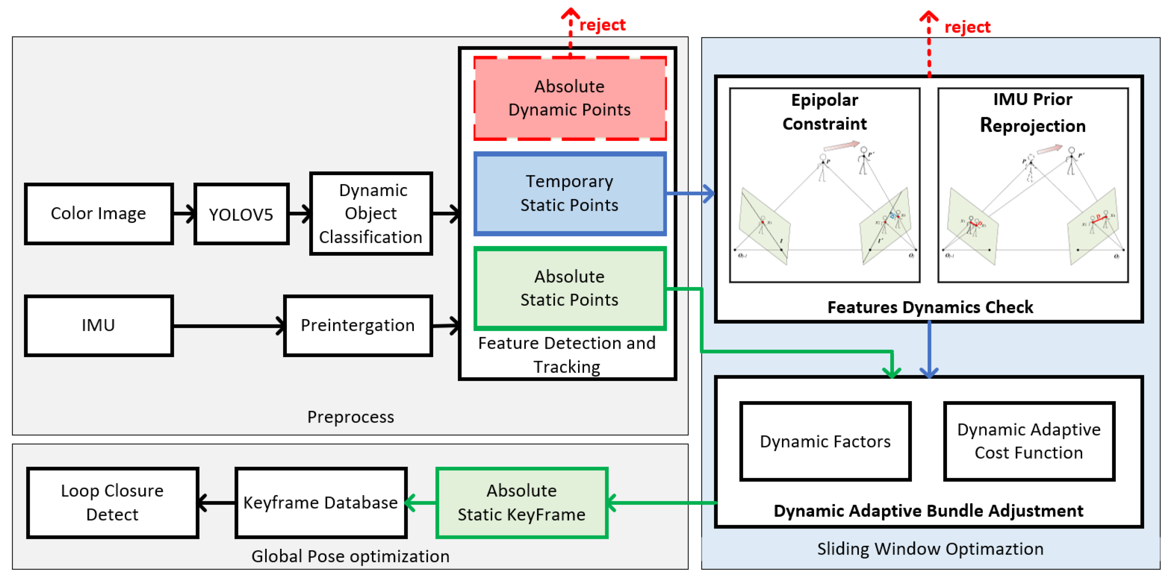
Figure 2.
Dynamic object hierarchy. The common objects in the COCO dataset are classified based on life experience, The higher the level, the higher the potential motion of the object. I and II are considered as static objects, III and IV are considered as temporary static objects, and V is considered as dynamic objects.
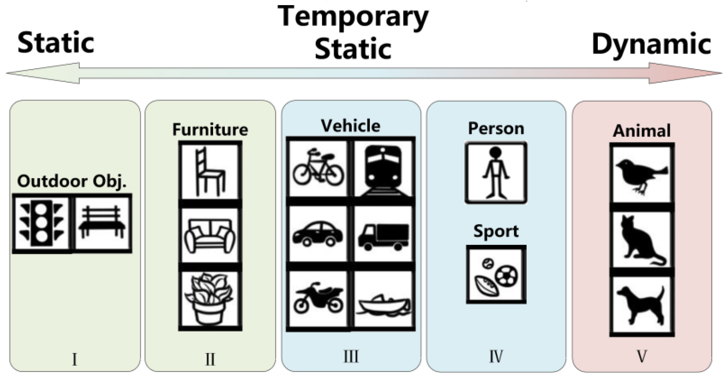
Figure 3.
Reprojection error based on IMU prior constraint for temprary static points. (a) Reprojection process with IMU pre-intergration. (b)A special case for moving toward the optical center Oj. The red line represents the reprojection error. The short dashed line indicates that the object is static. For convenience of viewing, green and red line represent the overlapping parts, in (b).
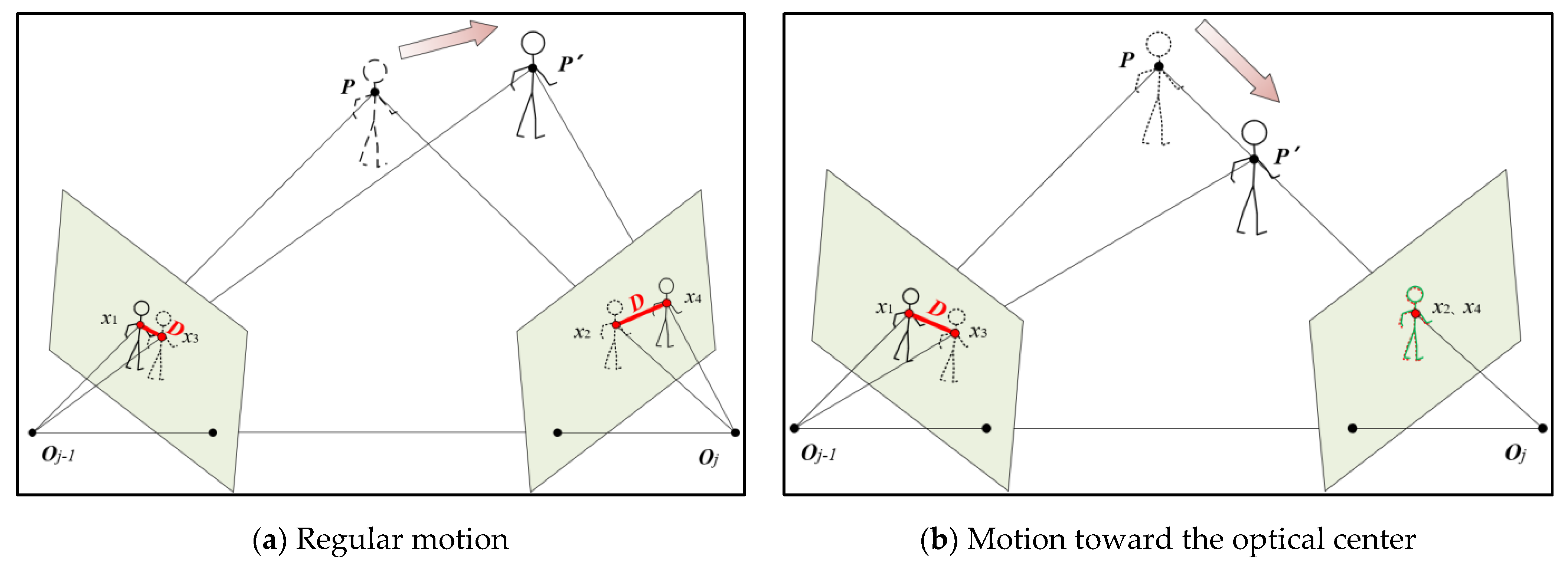
Figure 4.
Epipolar constraint for temprary static points. (a) Epipolar constraint in regular cases. (b)A special case for moving toward the optical center Oj-1. The blue line represents the distance between feature point to its epipolar line. The short dashed line indicates the epipolar lines.
Figure 4.
Epipolar constraint for temprary static points. (a) Epipolar constraint in regular cases. (b)A special case for moving toward the optical center Oj-1. The blue line represents the distance between feature point to its epipolar line. The short dashed line indicates the epipolar lines.
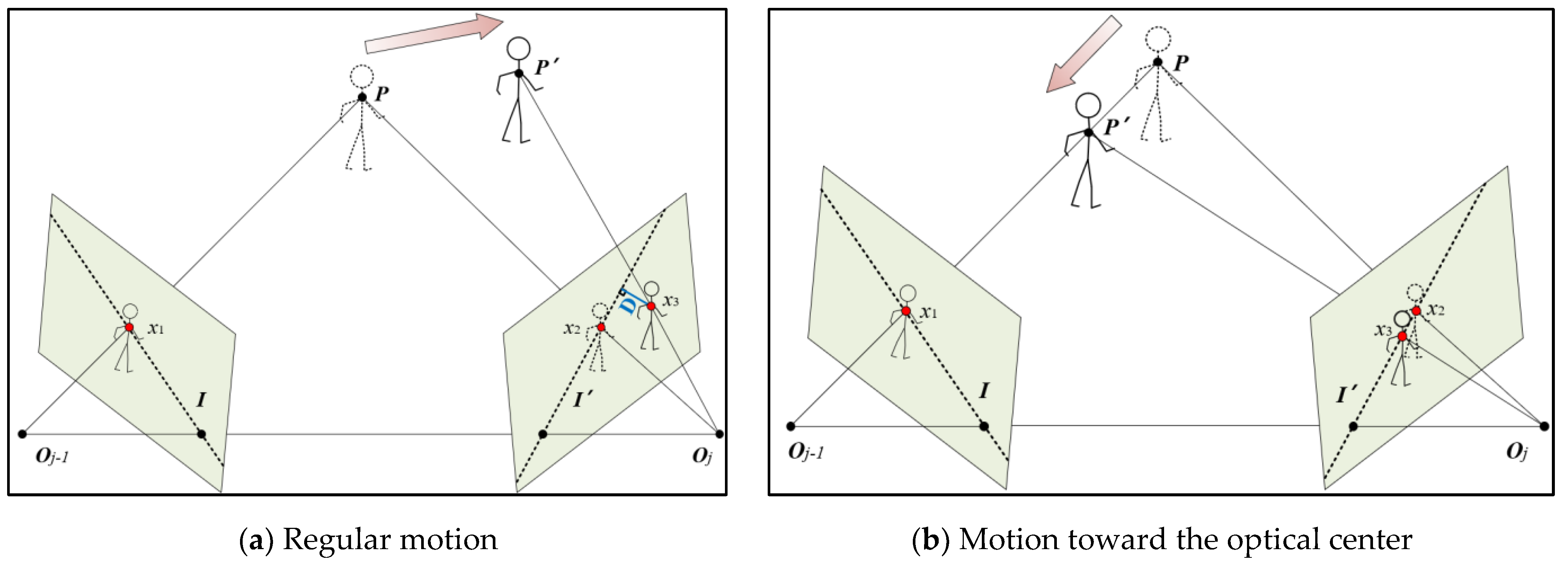
Figure 5.
Comparison trajectories results of D-VINS (blue) and ORB-SLAM2 (green) in TUM datasets. (a)-(g) are the trajectory comparison results for each sequence of the TUM RGB-D dataset. (h) is the comparision results for the two algorithms of the fr3_walking_rpy sequence. Horizontal axis represents time in seconds, and the longitudinal axis represents the ATE in meters.
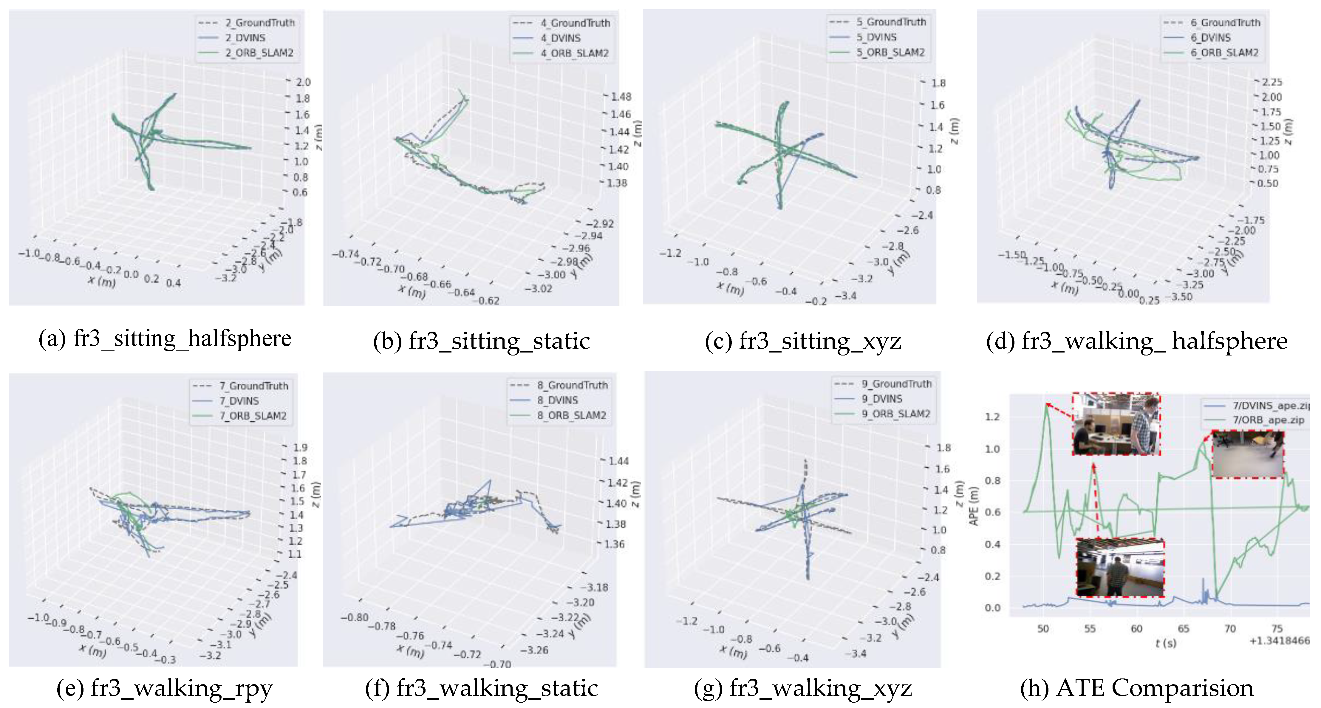
Figure 6.
Comparison trajectories results of VINS-Fusion, DynaVINS and D-VINS in KITTI 05 and 07 sequences. (a), (b)represent the accuracy heat maps and comparison results for the 05 sequence and (c), (b) is for 07 sequence, respectively.
Figure 6.
Comparison trajectories results of VINS-Fusion, DynaVINS and D-VINS in KITTI 05 and 07 sequences. (a), (b)represent the accuracy heat maps and comparison results for the 05 sequence and (c), (b) is for 07 sequence, respectively.
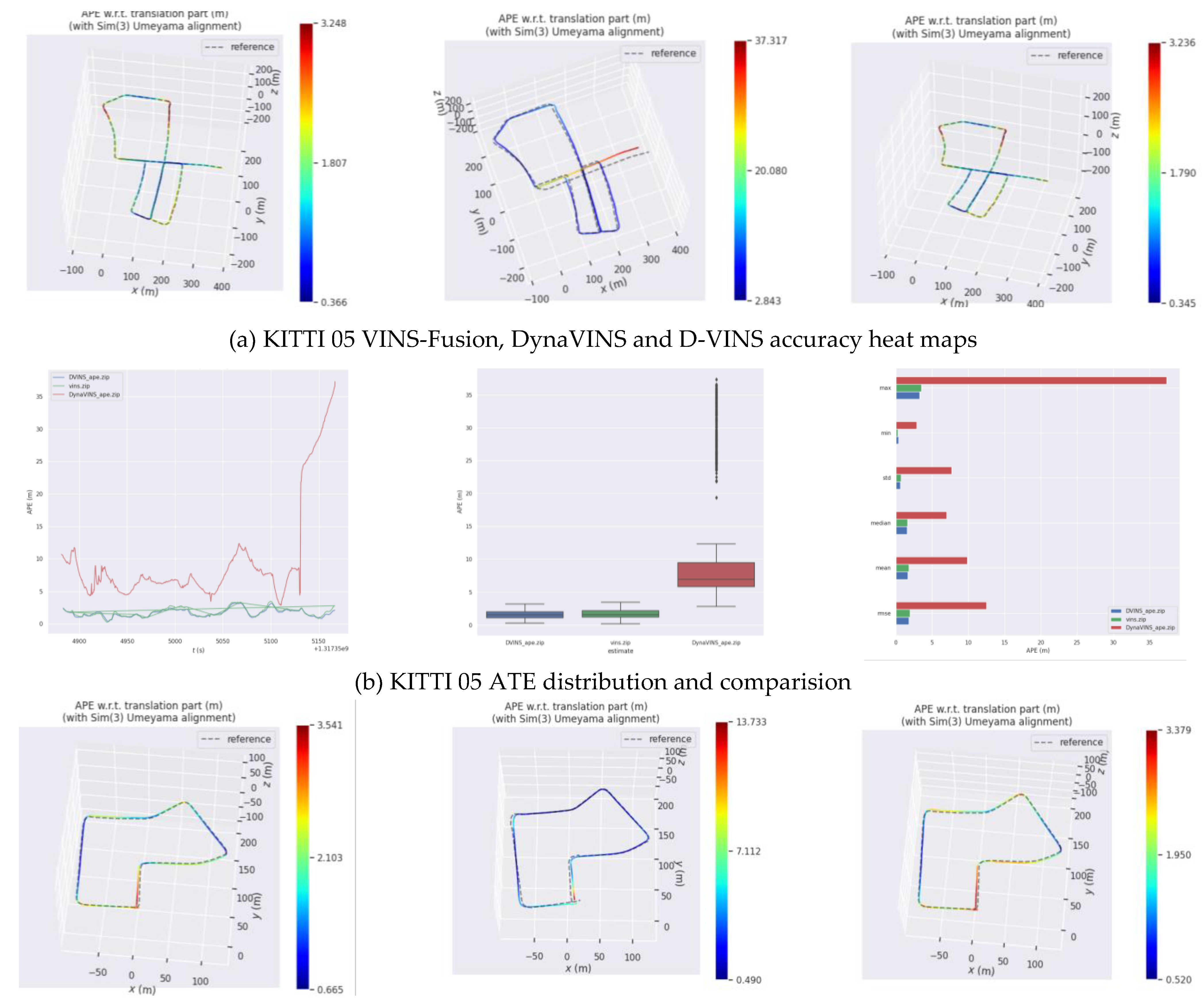
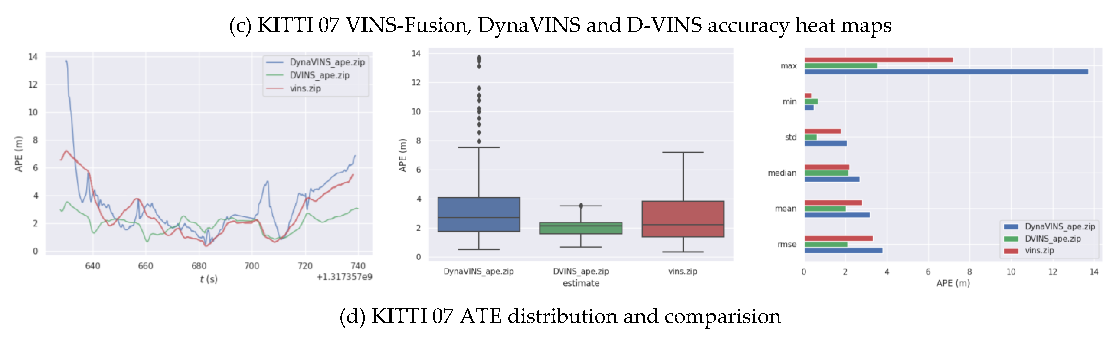
Figure 7.
Result of trajactory and detection of VINS-Fusion, DynaVINS and D-VINS in VIODE dataset(parking_lot, city_day and city_night scenes).In (a), (c) and (e), the first three figures are ATE distribution of 0_none, 1_low, 2_mid, and 3_high sequences and the last figures are the trajactory of three algorithms in 3_high sequence. In (b), (d) and (f), the first three figures demonstrate features dynamics check result, where green points are absolute static points, purple points are temporary static points and white points are absolute dynamic points.The last figures are the bounding box from YOLOV5.
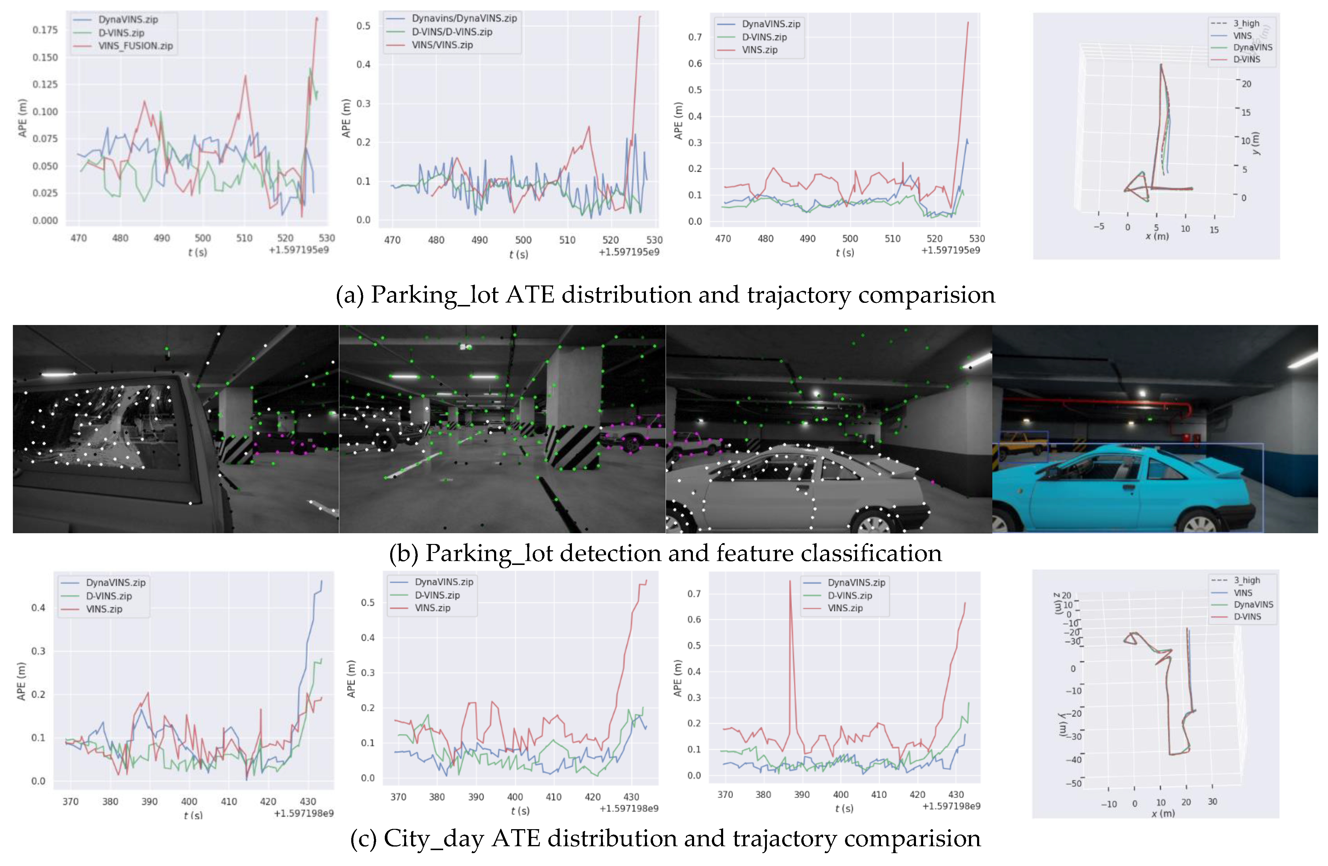
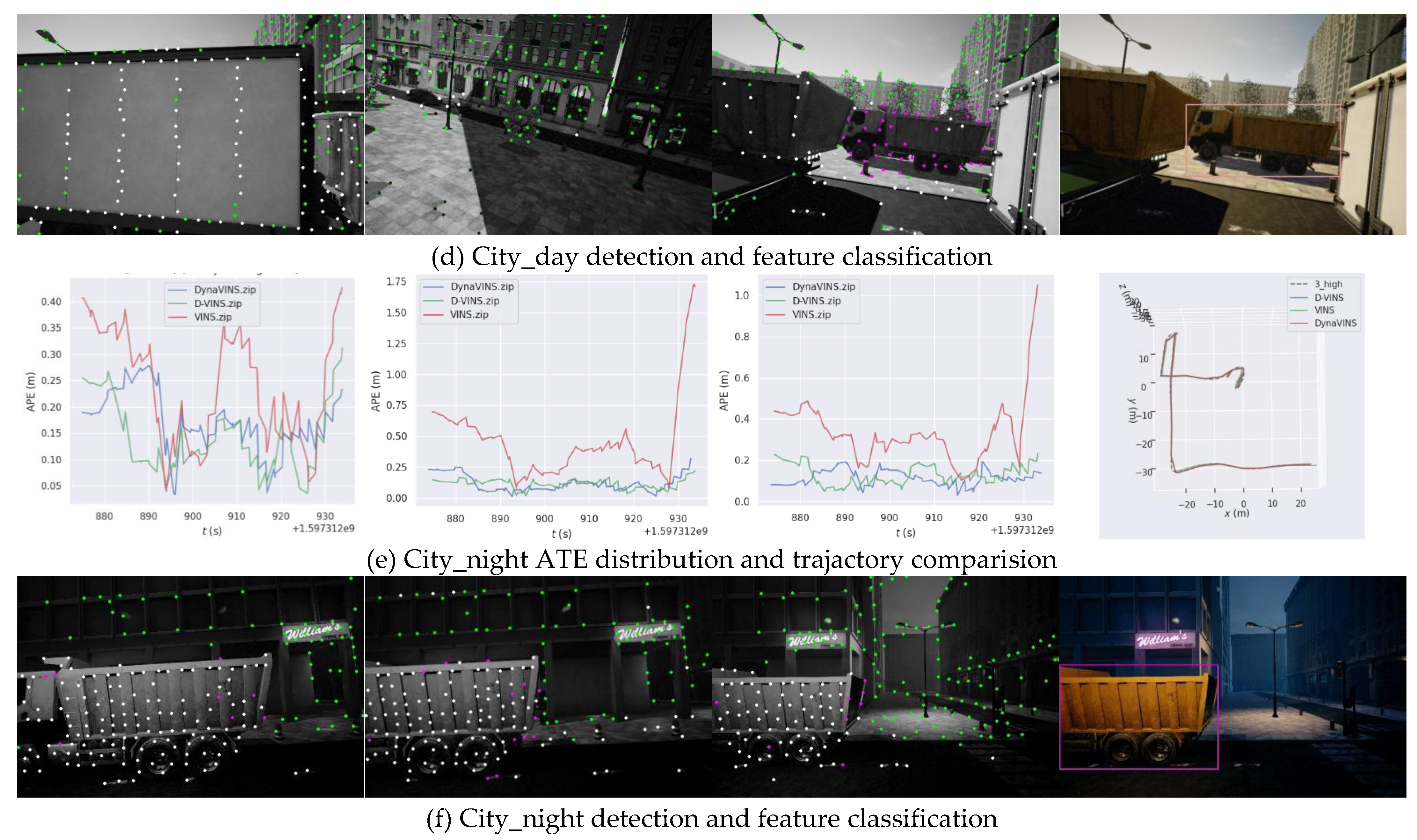
Figure 8.
handheld/backpack data collection equipment. (a) shows the overall of the equipment. (b) shows the handheld part. (c) shows the backpack part. (d) and (e) show the data collection work with different mode.
Figure 8.
handheld/backpack data collection equipment. (a) shows the overall of the equipment. (b) shows the handheld part. (c) shows the backpack part. (d) and (e) show the data collection work with different mode.
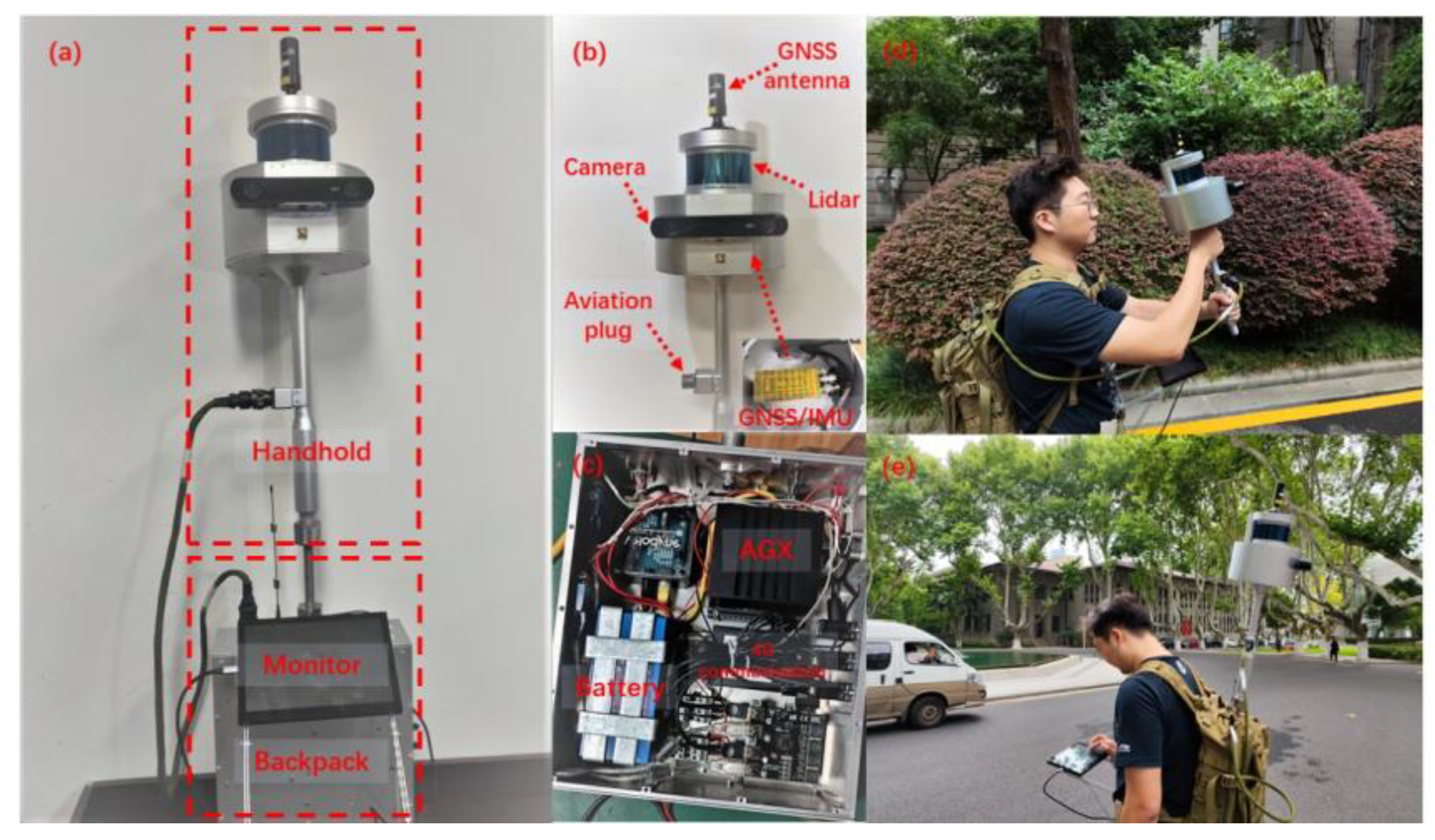
Figure 9.
Feature classification results in our datasets. (a) shows 5_SLAM_country_dynamic_loop_1 sequence. (b) shows 14_SLAM_car_road_1 sequence. (c) shows 18_SLAM_car_road_2 sequence. Features in white are absolute dynamic points, those in green are absolute static points and those in purple are temporary static points.
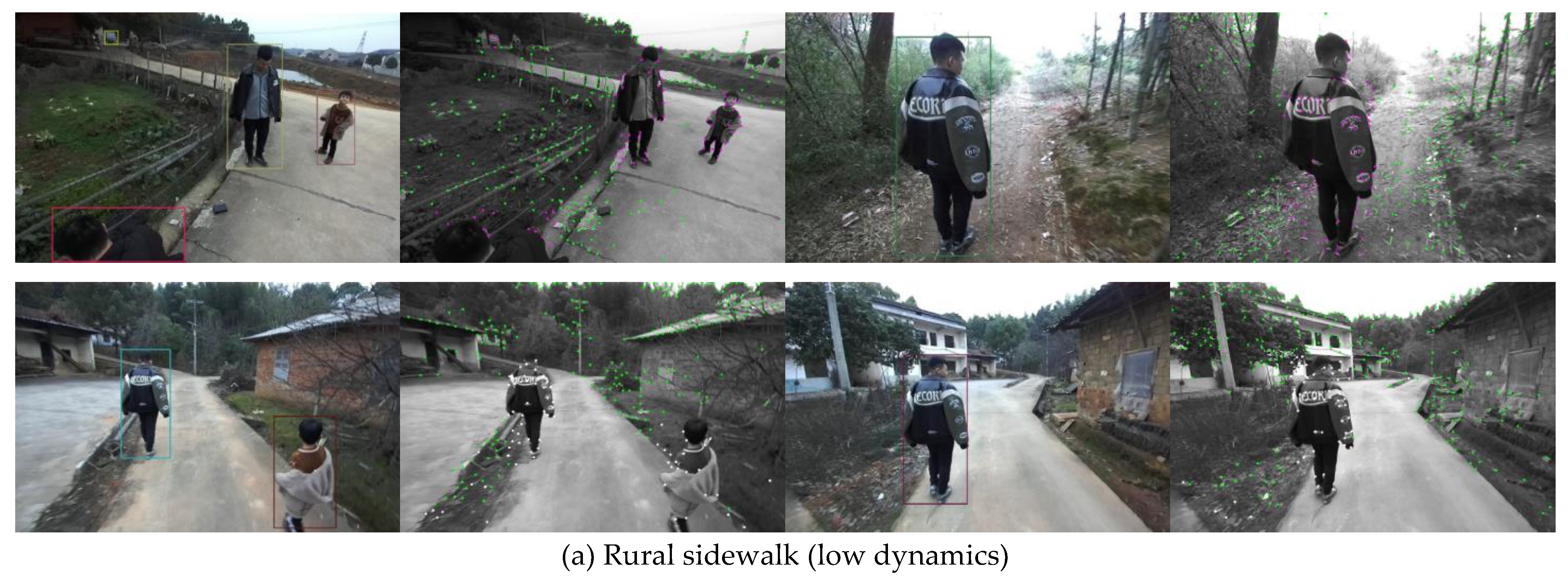
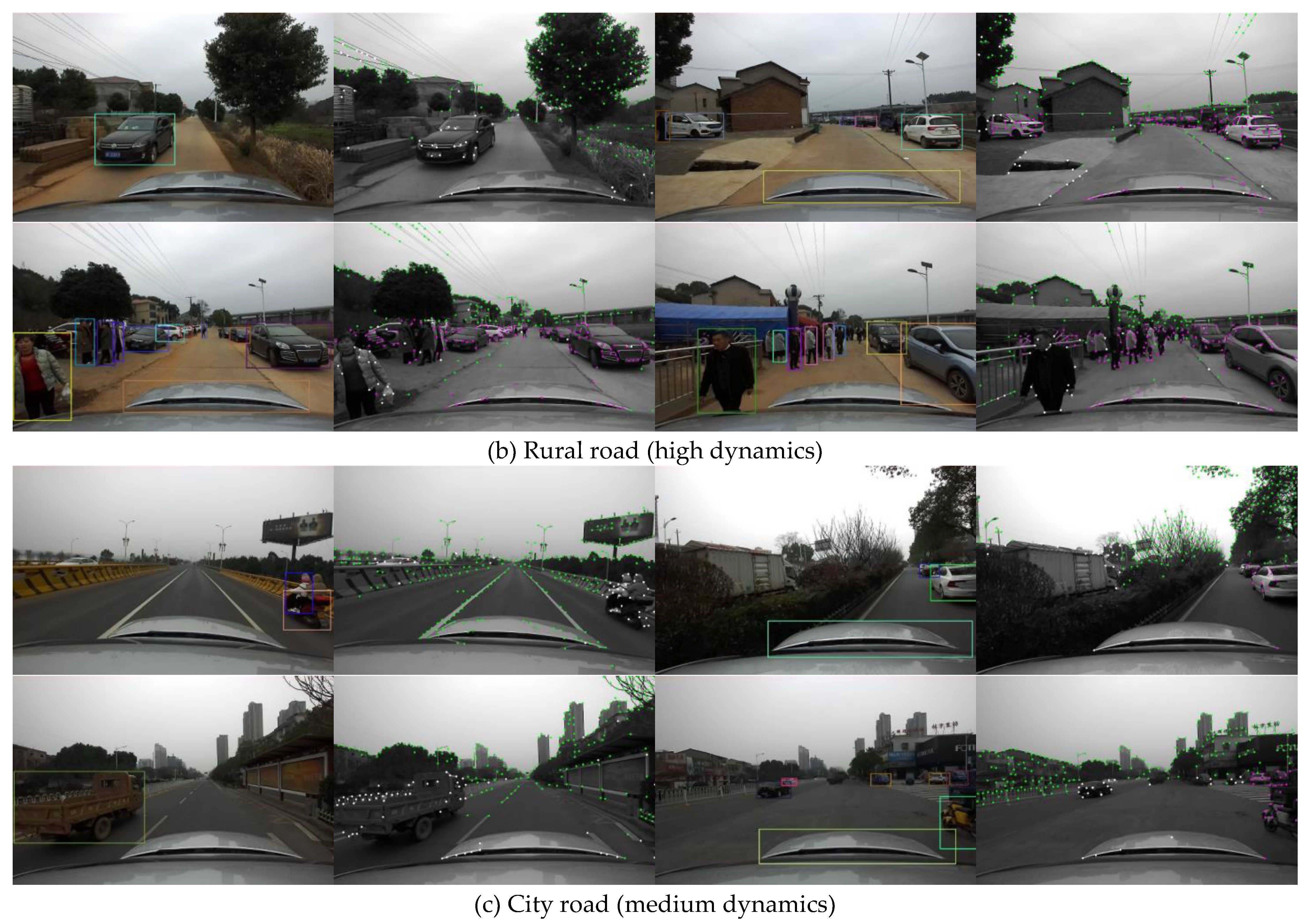
Figure 10.
APE distribution results in our datasets. (a) shows 5_SLAM_country_dynamic_loop_1 sequence. (b) shows 14_SLAM_car_road_1 sequence. (c) shows 18_SLAM_car_road_2 sequence. DynaVINS failed to estimate in 14_SLAM_car_road_1 and 18_SLAM_car_road_2 sequence, so it was not compared in those sequences.
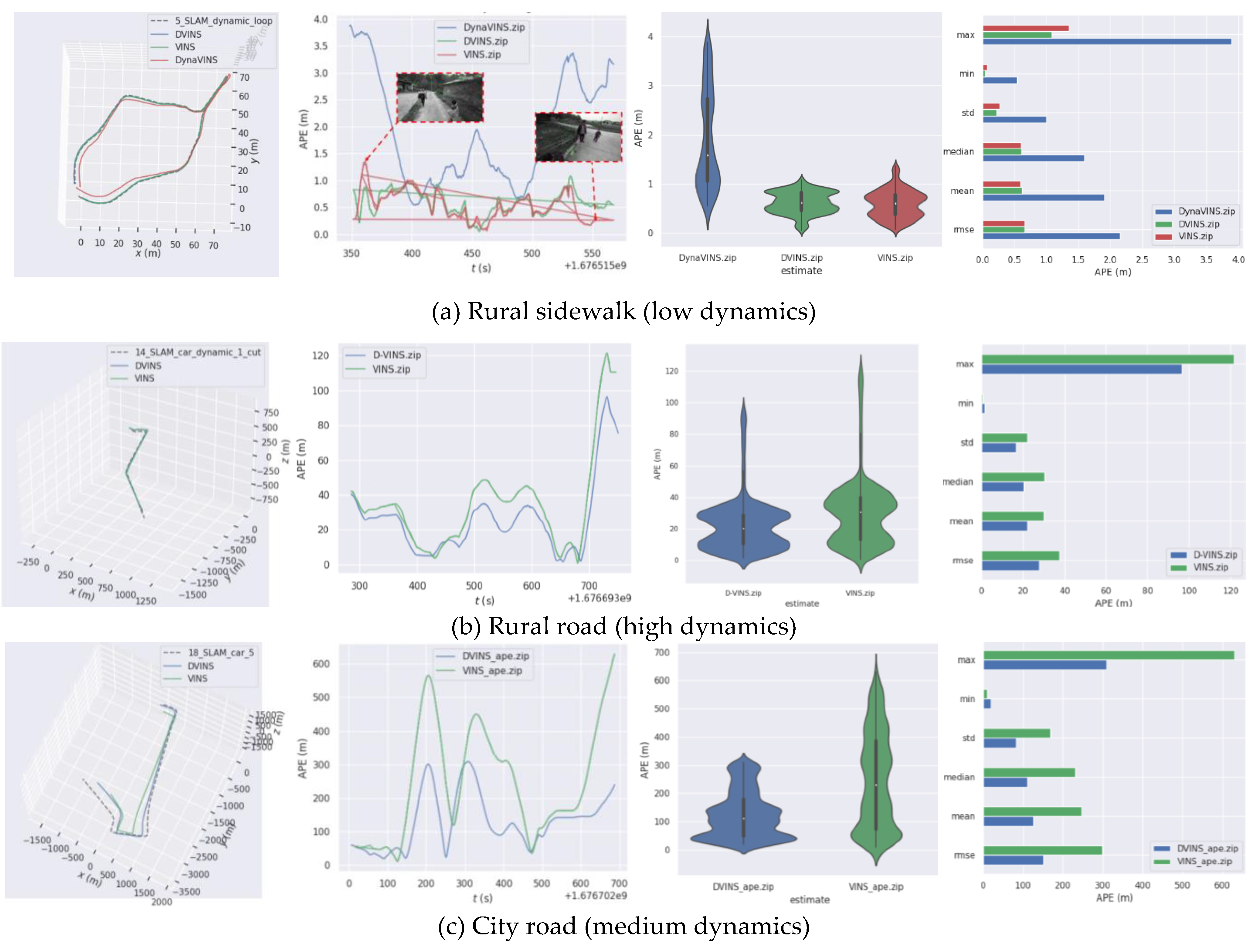

Table 1.
The ATE and RPE RMSE (m) of ORB-SLAM2 and D-VINS in TUM RGB-D dataset.
| Sequences | ORB-SLAM2 | D-VINS* | Improvement | |||
|---|---|---|---|---|---|---|
| ATE | RPE | ATE | RPE | ATE | RPE | |
| fr3_sitting_static | 0.0116 | 0.0152 | 0.008 | 0.0114 | 31.03% | 25.00% |
| fr3_sitting_xyz | 0.0133 | 0.0199 | 0.0153 | 0.0179 | - | 10.05% |
| fr3_sitting_halfsphere | 0.0336 | 0.0124 | 0.0252 | 0.0122 | 25.00% | 1.61% |
| fr3_walking_static | 0.4121 | 0.0299 | 0.0069 | 0.0101 | 98.32% | 66.22% |
| fr3_walking_xyz | 0.8856 | 0.1255 | 0.0155 | 0.0182 | 98.24% | 85.49% |
| fr3_walking_rpy | 0.5987 | 0.0528 | 0.0422 | 0.0432 | 92.95% | 18.18% |
| fr3_walking_ halfsphere | 0.4227 | 0.0338 | 0.0216 | 0.0234 | 94.89% | 30.77% |
Note: ”*” indicates that D-VINS removed the module containing IMU. Symbol "-" indicates that the algorithm has no improvement.
Table 2.
The ATE RMSE(m) of VINS-Fusion, DynaVINS and D-VINS in KITTI dataset.
| Sequences | VINS-Fusion | DynaVINS | D-VINS |
|---|---|---|---|
| KITTI 05 | 1.913 | 12.4668 | 1.7631 |
| KITTI 07 | 2.1927 | 3.8006 | 2.1100 |
Note: Bold letters indicates the best results.
Table 3.
The ATE RMSE(m) of VINS-Fusion, DynaVINS and D-VINS in VIODE dataset.
| Scenes | Sequences | VINS-Fusion | DynaVINS | D-VINS |
|---|---|---|---|---|
| Parking_lot | 0_none | 0.0774 | 0.0595 | 0.0538 |
| 1_low | 0.1126 | 0.0826 | 0.0472 | |
| 2_mid | 0.1174 | 0.0630 | 0.0396 | |
| 3_high | 0.1998 | 0.0982 | 0.0664 | |
| City_day | 0_none | 0.1041 | 0.1391 | 0.0882 |
| 1_low | 0.2043 | 0.0748 | 0.0912 | |
| 2_mid | 0.2319 | 0.0520 | 0.0864 | |
| 3_high | 0.3135 | 0.0743 | 0.0835 | |
| City_night | 0_none | 0.2624 | 0.1801 | 0.1561 |
| 1_low | 0.5665 | 0.1413 | 0.1221 | |
| 2_mid | 0.3862 | 0.1192 | 0.1395 | |
| 3_high | 0.7611 | 0.1519 | 0.1566 |
Note: Bold letters indicates the best results.
Table 4.
The ATE RMSE(m) of VINS-Fusion, DynaVINS and D-VINS in KITTI dataset.
| Sequences | VINS-Fusion | DynaVINS | D-VINS |
|---|---|---|---|
| 5_SLAM_dynamic_loop_1 | 0.657039 | 2.145493 | 0.654882 |
| 14_SLAM_car_road_1 | 37.31964 | - | 27.60877 |
| 18_SLAM_car_road_2 | 299.7889 | - | 151.2075 |
Note: “-” indacates that the method failed to estimate camera pose. Bold letters indicates the best results.
Disclaimer/Publisher’s Note: The statements, opinions and data contained in all publications are solely those of the individual author(s) and contributor(s) and not of MDPI and/or the editor(s). MDPI and/or the editor(s) disclaim responsibility for any injury to people or property resulting from any ideas, methods, instructions or products referred to in the content. |
© 2023 by the authors. Licensee MDPI, Basel, Switzerland. This article is an open access article distributed under the terms and conditions of the Creative Commons Attribution (CC BY) license (http://creativecommons.org/licenses/by/4.0/).
Copyright: This open access article is published under a Creative Commons CC BY 4.0 license, which permit the free download, distribution, and reuse, provided that the author and preprint are cited in any reuse.


