
Submitted:
26 May 2023
Posted:
31 May 2023
You are already at the latest version
Abstract
Evaluating the economic impact of airports is crucial for understanding the benefits they bring to a region. However, when an area has more than one airport, it becomes essential to analyze each airport's contribution to the local economy to make informed investment and policy decisions. Thus, studying economic models that can distinguish each airport's impact on the region's economy becomes essential. In this context, this paper aims to compare three different approaches to determine the economic contribution of airports in a given region and identify their social and economic benefits. The International Civil Aviation Organization recommends using Input-Output analysis in this context. The study considered three weight factors for the Input-Output basic model: circular buffer, displacement time, and Huff's gravitational model. The analysis was performed using the three largest airports in São Paulo's state, Brazil, due to their proximity and influence on the surrounding area. The models were compared based on their efficiency and accuracy in reflecting the reality of the case study context. The study identified the most suitable model for establishing correlations between investments made in airport infrastructure and the generation of gross domestic product, employment, and added value. This study fills a gap in the existing literature by proposing improvements to the methods for evaluating airports' economic and social benefits. In recent times, airport investors, both in the government and private sectors, have become increasingly demanding in their need for accurate analyses before making investments. Therefore, the results of this paper will provide valuable insights into the benefits of investing in airport infrastructure and help policymakers and investors make informed decisions.
Keywords:
Economic Impacts of Airports
; Airport Investments
; Input-output analysis
; Data Science
1. Introduction
The presence of airport infrastructure directly impacts its surrounding areas’ economic and social development. It is well known that the local economy’s generation of Gross Domestic Product (GDP) benefits several sectors and leads to regional growth. The Input-Output model, also known as Input-Output tables, can be applied to analyzing the air transport sector in a given region. This methodology is recommended by the International Civil Aviation Organization (ICAO) to assess the economic impacts of airport infrastructure. However, the presence of more than one airport in the same region can lead to a problem of overlapping airport interference.
Analysis models have been developed for overlapping regions with airports in common areas to address this issue. These methods can help with the economic analysis of a given airport. Furthermore, the presence of airport infrastructure with more than one airport can influence the development of a region, which can be measured through its economic effects and social indicators.
Thus, three models will be used to analyze the economic effects of airport infrastructure in regions with an overlap of airport interference. The deterministic and static models consider physical parameters such as distance and user travel time to the airport [1]. On the other hand, probabilistic models prioritize factors such as airport attractiveness, travel time, and passenger and air cargo movement, among other factors. These models aim to identify the most suitable model to identify correlations between investments made and the generation of GDP, employment, and added value.
Air transport significantly impacts the economy, as it involves several sectors of economic structures and the transport sector itself. The impact of air transport can be evaluated by considering the gains and losses in other sectors of the economy. The input-output (IO) model is a valuable tool for analyzing the regional impacts of air transport. The IO model has several advantages, including considering industrial interdependence and defining transport as input and output sectors [2]. Using the IO model, it is possible to identify how the impacts are aggregated and distributed differently among economic sectors and to model specific sectors without causing direct changes in others. However, IO modeling can be very complex, especially in small regions.
Overall, the IO model helps assess the economic effects of air transport in a region by considering the interconnections among different sectors of the economy. This allows for a more comprehensive analysis of the economic impacts of air transport, including its contribution to GDP, employment, and added value. Nevertheless, the IO model requires careful consideration of several parameters, such as the regional context and data availability, to ensure accurate results.
Air transport plays a crucial economic role by impacting various sectors and the overall financial structure. Therefore, it is essential to recognize both the positive and negative impacts of air transport on the economy. The input-output (IO) model is a valuable tool for analyzing the regional effects of air transport. This model has several advantages, including capturing the interdependence of different industries and defining the transport sector with input and output sectors. In addition, the IO model can help identify how the impacts of air transport are distributed across different economic sectors, and it allows for specific modeling of certain sectors without causing direct changes in others.
The input-output (IO) model helps identify how impacts are aggregated and distributed across different economic sectors. It also allows for specific modeling of certain sectors without causing direct changes in others. However, it is essential to note that IO modeling can be very complex, especially in small regions.
While the IO model has advantages such as industrial interdependence and defining the transport concept with input and output sectors, it only partially represents the economy and may lead to inconsistent and inaccurate estimates if the simplification of actual savings is not considered. When analyzing and quantifying the effects of multipliers in the air transport sector, it is essential to consider the three most common indicators for the IO model: product and income [3].
This paper presents an alternative methodology to better utilize Input-Output data in regions that have multiple airports. The proposed methodology employs probability distributions as weight factors to divide the input-output air transport economic data. These distributions are based on both deterministic and probabilistic approaches. The proposed methodology is suitable for predicting returns on investments in the air transport sector, thus enabling decision-makers and policymakers to make informed investment decisions. Furthermore, by using this methodology, investments in the air transport sector can be optimized, leading to improved economic outcomes. Overall, this work contributes to the literature by presenting a novel methodology that can be used to better leverage Input-Output data in regions with multiple airports. The proposed methodology has practical applications and can help decision-makers and policymakers allocate investments more effectively in the air transport sector.
The following section will review the literature on using IO tables for the development and growth of the air transport sector. Section 3 will describe the methodology for applying the input-output model and the three weight models (circular buffer, displacement time, and the Huff model) to be used. Section 4 will present the analysis results, and section 5 will provide the conclusion.
2. Literature Review
The air transport sector has garnered increasing attention from researchers in recent years, leading to numerous studies proposing models for evaluating its economic impact in specific regions. One effective method for analyzing the air transport sector in a particular area is through the Input-Output (IO) approach, also known as IO tables or IO model.
The IO model provides a standardized method for tracking the flow of goods and services between different sectors of a country’s economy and its component sectors. This statistical breakdown of the other economic sectors allows for a comprehensive analysis of the impacts of air transport on the economy [4]. While several economic and econometric approaches can be employed to assess the effects of the air transport sector on the economy, the IO model is an approach that quantifies the direct, indirect, and induced impacts of air transport on the national economy [5].
For instance, Tveter [6] proposed a difference-in-difference Input-Output model to account for population growth resulting from regional airports. Tveter estimated the effects of regional airports using data from airports in Norway between 1970 and 1980. In addition, the study accounted for the level of economic development observed in the cities located around the airports. The proposed model is a valuable contribution to the literature, as it provides a rigorous method for estimating the economic impacts of regional airports. Furthermore, by using a difference-in-difference approach, the model controls for the factors that may affect the outcomes of interest, such as population growth. Overall, Tveter’s work highlights the importance of accounting for population growth in estimating the economic impacts of regional airports. In addition, by considering the level of economic development in the surrounding cities, the model provides a more accurate picture of the effects of airports on the local economy.
Nasution et al. [5] identified a relationship between air transport and economic growth in Indonesia, connecting the data on passenger/air cargo movement and GDP. One of the main reasons related to the GDP growth of a given region may be associated with the investment or expansion of the airport for passengers or its air cargo capacity. The implications could even generate development in the cities near and around the airport. Some consequences of the airport investment can be noted, such as job openings, increased revenue associated with the airport, economic benefits in the area since the beginning of the airport operations, and the impact stimuli of companies from different airlines and even those that offer services directly for air transport [5].
Yu [7] used economic and econometric impact models to describe IO modeling and IO model applications, including single and multi-region models. Aden [8] explains that the acceleration of city growth depends mainly on factors such as better use of the country’s potential and sustained and planned action for new priority sectors that create wealth and employment. Thus, improving the infrastructure implemented in the territory provides qualities and measures of economic, administrative, and governmental incentives.
Bagoulla e Guillotreau [9] analyzed maritime transport in France using Input-Output (IO) tables to measure the effects of this mode of transportation on product and employment generation. The study highlights the usefulness of the IO approach in evaluating the economic impacts of transportation sectors. The IO model provides a standardized method for tracking the flow of goods and services between different sectors of a country’s economy and its component sectors. By employing this approach, these authors were able to quantify maritime transport’s direct and indirect impacts on the French economy, particularly regarding product and employment generation. Furthermore, the study showcases the adaptability of the IO model for specific applications, such as evaluating transportation sectors. It provides a comprehensive and standardized framework for analysis. The IO model can aid policymakers and researchers in identifying the economic impacts of various sectors and developing effective policies to support their growth.
Subanti et al. [10] conducted a study to identify the interregional effects associated with different transport means in Indonesia. The authors employed the Inter-Regional Input-Output (IRIO) model to achieve this. The IRIO model is a specialized version of the Input-Output (IO) model, which accounts for the interdependence between different regions in an economy. The authors also quantified the direct and indirect impacts of different modes of transportation on the Central Java province’s economy while accounting for the interregional effects. The study highlights the usefulness of the IRIO model in evaluating the economic impacts of transportation sectors in a region while accounting for the interdependence between different regions.
Bandeira et al. [11] proposed a methodology based on input-output (IO) tables to determine the economic impact of Viracopos Airport in the metropolitan region of Campinas, Brazil. The study employed the IO model to assess the direct and indirect effects of the airport’s activities on the local economy. Using this approach, the authors compared the performance of Viracopos Airport with the financial performance of the city and the Brazilian national economy. By analyzing the airport’s contributions to gross domestic product (GDP), employment, and added value, the study provided insights into the airport’s economic impact on the region. The proposed methodology offered a valuable framework for assessing the economic impact of airports and other transportation sectors on the local economy, which can help policymakers and investors make more informed decisions about infrastructure investments. The study highlighted the importance of employing the IO model to quantify the economic benefits of transportation infrastructure, such as airports, and develop effective policies for sustainable growth.
Keček et al. [12] conducted a macroeconomic analysis of the transport sector and its impact on employment. The authors examined the contributions of air, land, and maritime transport sectors to the employment multiplier, which measures the number of jobs created for each input unit. Their findings indicate that the transport sector, including air, land, and maritime transport, has a significant impact on the employment multiplier, suggesting that investments in transportation infrastructure can generate substantial employment benefits. Their results underscored the importance of the transport sector as a key driver of economic growth and job creation. The study highlighted the value of conducting macroeconomic analyses to understand the broader economic impacts of transportation infrastructure investments, which can inform policy decisions and guide investments in the sector. By providing insights into the employment benefits of the transport sector, the study contributes to a better understanding of the role of transportation infrastructure in promoting sustainable economic development.
Mishra et al. [13] conducted a study to assess the economic links between air traffic and 15 states in India. The authors analyzed the impact of air transportation on economic activity and productivity and its role in promoting regional development. Their study provides valuable insights into the economic benefits of air transportation in India, highlighting its potential to boost economic growth and development. The authors’ findings suggest that investments in air transportation infrastructure can lead to increased trade, investment, and tourism, generating positive spillover effects for the wider economy. The study underscores the importance of understanding the economic links between air traffic and regional development, particularly in emerging economies like India, where transportation infrastructure plays a critical role in facilitating economic growth. Furthermore, by shedding light on the economic impacts of air transportation, the study contributes to a better understanding of the role of transportation infrastructure in promoting sustainable economic development.
The IO model has been widely recognized as an essential tool for analyzing the economic impacts of the air transport sector in a given region. Several studies have proposed alternative methodologies for assessing airports’ growth, development, and economic impact in areas of interest. These methodologies include using probability distributions as weight factors for dividing input-output air transport economic data, analyzing inter-regional effects associated with means of transport, and employing the difference-in-difference input-output model to account for population growth due to regional airports.
Overall, the IO model provides a standardized approach for evaluating the air transport sector’s direct, indirect, and induced impacts on a national or regional economy. By applying various economic and econometric methods, researchers can understand the economic benefits of air transportation and inform policy decisions that promote sustainable economic development. Table 1 systematically reviews work on the input-output model and economic growth.
3. Methodology
The data analysis was conducted in the following order: first, the airports were selected, and then the municipalities within a 200km radius were identified. Next, the IO tables were analyzed to obtain economic data for these cities. The IO analysis determined two average multipliers: generated product and generated income. After obtaining the average multipliers, three distribution models were applied: the circular buffer model, travel time model, and Huff’s model. Finally, the individual contribution of each airport was determined based on the results obtained from applying the distribution models.
Figure 1 presents the flowchart that defines the steps developed in this work. The grey rectangles offer the methodological work stages, the green ones the models adopted in the research, and the red ones the names of the variables that result from the work.
It should be noted that in the analysis of weight models for the input-output method, municipalities located within a 200 km radius of the airport will be considered. Thus, the analysis will be based on the same number of municipalities for all three models. However, each city will have a different weight depending on the methodology adopted by each model.
Input-Output Method
The IO-Tables method consists of three matrices: the matrix of intersectoral flows (S-table), the matrix of technical coefficients (A-table), and the matrix of intersectoral impacts (L-table), or the Leontief matrix.
Table S considers the entire economy disaggregated into N sectors, represented in an NxN arrangement of a square matrix referring to the sectors, plus other inputs (inputs, imports, taxes, and profit margins) and other outputs (exports, government, and final consumers). The sums of the rows and columns for each sector represent, respectively, the total demand and production in a given period. The vectors for total demand and production are equal, indicating the equilibrium state of the economy (LEONTIEF, 1986).
Table L is obtained by Equation 1. This matrix contains multipliers for calculating the indirect effects (L) of each sector in the economic system.

Where I is the identity matrix, and the matrix L is the inverse of the difference between the identity matrix I and table A. It is called the L table or Leontief Matrix, simplifying the linear system notation according to Equation 2:

The Y vector consolidates the exogenous demand (consumption) data to the sectors that build the A-table to calculate the vector X of production needed to meet such a demand.
The L-table has the same dimension as the A-table and positive numerical coefficients, eventually greater than 1, called economic impact multipliers, given their algebraic form in determining the effects of demand variation on supply. This relationship is the basis for several analyses and conclusions from the input-output matrices, particularly direct and indirect impact measures.
Impact multipliers are powerful analytical tools associated with input-output matrices. They are dimensionless coefficients that represent the effects in response to any change imposed on an economic system in equilibrium. A measure of an economic sector’s "quality" or "strategic" nature is also used to describe its ability to multiply effects on the economy. Sectors with high multipliers are considered the most relevant because they can trigger more effects on a given expenditure in the face of an incentive.
By definition, a multiplier is calculated based on the hypothesis of adding one unit to the demand of a given sector, assuming that external needs for the rest of the economy remain unchanged. In this sense, for the results of this study, it is considered that the initial effect generated by the increase of one more unit in the demand of a given sector (j) will cause the need for one more unit of products in this sector. In this logic, the "direct impact" is evident, as one more unit of demand will produce one more unit of product, that is, xj = 1.
It should be considered that the total effect propagates because of the interdependence between sector j and the other sectors of the economy. The greater this interdependence, the more significant the total impact. Thus, it can be seen that if sector j is hypothetically wholly isolated from the rest of the economy, the total effect will be equal to the initial impact. For this reason, the full product includes the initial development, that is, it is the sum of the direct impact with the indirect impacts, where (Equation 3):

Therefore, ∆x is the "total effect", meaning the change in production in all sectors of the economy due to the initial effect in a given sector j. In short, the total impact captures the spread of the initial development to the rest of the economy.
Finally, it is worth mentioning that the estimates of the multipliers calculated by the Leontief matrix in this study follow the economy modeled by the input-output matrix, thus assuming general equilibrium properties [3,4].
The IO-Tables application requires official databases on the country’s economy. Therefore, it was essential to extract these data to assess the economics of the air transport sector in the area of influence of airports. Thus, to obtain the input-output matrices, the following banks were consulted:
- IO-Tables System for the National Economy: The Center for Regional and Urban Economics of the University of São Paulo (NEREUS) annually publishes good approximations of the IBGE matrices [14], which in turn publishes them every five years. These matrices are calculated according to the recommendations of the Brazilian System of National Accounts.
- IO-Tables system for the region of study: In the Brazilian case, the primary source of information for constructing the location quotient vector is the data referring to the work factor [11]. The Federal Government provides detailed micro-data on employment and wages, described individually by workers and indexed by sector of economic activity and municipality. Following the methodology described by [15], it was possible to generate the location quotient vector for the S table of the 68 industries and obtain the regionalized IO-Tables. The total remuneration of the labor factor provides good quality regional specialization indexes better than if they were obtained only by the number of jobs, especially in a country with solid regional inequalities, such as Brazil [15].
Distribution Models for the input-output
The input-output method can be utilized to analyze regions with multiple airports by employing a weighted analysis of the attractiveness of each airport, as discussed by Wang et al. [16]. In such cases, the Leontief matrix’s weights can be determined by either a deterministic or probabilistic model proposed by Huber and Rinner [17]. Deterministic models are used when the airports in the study area have similar attractiveness and are based on physical parameters such as distance radius and displacement time to the airport. Two examples of deterministic models are the circular buffer and displacement time models. On the other hand, probabilistic models consider factors such as airport attractiveness, travel time, and the number of flights. One example of a probabilistic model is the Huff model, which can be used to determine airport weights in the Leontief matrix.
In this study, we will apply the circular buffer, displacement time, and Huff models to determine the weights of the Leontief matrix for the airports in our region of interest. By considering various factors that impact the attractiveness of each airport, these models will help provide a more accurate analysis of the economic impact of the air transport sector.
Circular Buffer Models
The most common economic sharing analysis method is establishing a circle centered on the reference point [18]. This model allows an initial approximation of the radius of influence of each point of interest. However, circular buffers can be inaccurate in areas with natural faults, such as rivers, lakes, and mountains, or poor road connectivity [17]. In such cases, the area inside the circle may be inaccessible to users. Furthermore, it may slightly skew the results because, in this case, all cities within the operating radius will have a defined weight regarding the model’s center. This weight can be expressed by (Equation 4):
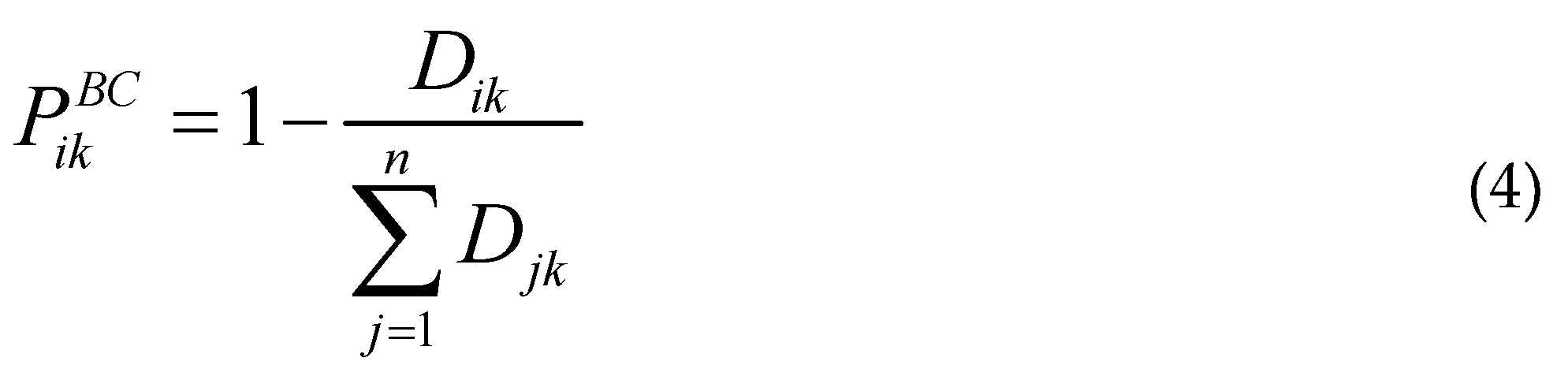
where PBC is the weight of the circular buffer model relative to the straight-line distance from airport i to city k, n is the number of airports impacting the city’s economy, and D is the distance to the airport. For better definition, the circular buffer model will analyze two airports in which the operating radius is estimated to be 200 km. In that case, the savings from air transport will be split between both airports.
Thus, the economic benefits of air transport for cities within the circular buffer zones will be allocated based on the Euclidean distance from the airports. Therefore, airports closer to the city will have a higher weight in the air transport sector’s impact on these cities’ economies.
Travel Time Models
Due to the limitation of circular buffers, some studies use travel time to define the economic share of the region [17]. This model represents reality better as it can predict natural limiting conditions such as the site’s topography. This analysis can be performed by calculating the distance to a given reference point through Google Maps.
Instead of using circular buffers, which have some limitations, some studies utilize travel time to determine the economic share of a region [17]. This model provides a more realistic representation of reality since it can account for natural limiting conditions, such as the area’s topography. The travel time analysis can be conducted by calculating the distance to a specific reference point using tools such as Google Maps [19].
The formulation of the time distance model is quite similar to the circular buffer model. However, the model employs the minimum travel time between the city and the airport instead of a straight-line distance. Thus, it can be written as (Equation 5):
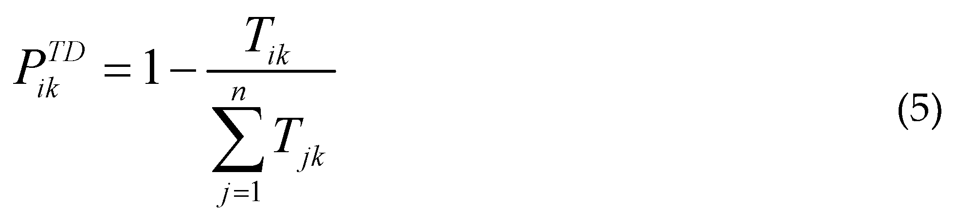
where PTD is the minimum travel time between city i and airport k, and T is the weight for the time distance model relative to city i and airport k.
Huff’s Gravitational Model
When multiple airports serve a common region, each of them can be considered to have a certain level of attractiveness to that region’s public. Therefore, academics and analysts extensively use the probabilistic model of spatial consumer behavior introduced by Huff in 1964 in various applications, including air transport [20,21]. Generally, the results obtained using Huff’s probabilistic model are more realistic than those obtained using deterministic models, as the former considers the variability in the attractiveness of each airport [17]. The model is based on the principle that the probability of a given consumer visiting and using a given location is a function of the distance from that location, its attractiveness, and the distance and attractiveness of other competing sites.
The popularity of Huff’s model can be attributed to its conceptual appeal, ease of handling, and applicability to a wide range of problems [20]. It is applied when one wants to understand the spatial behavior of a given population. The probability that a consumer located at point i will choose to go to an attractive point j is represented by Pij in this model (Equation 6):
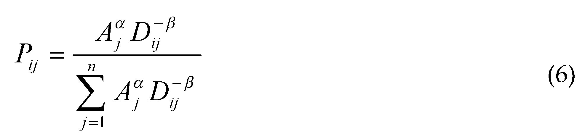
where Aj is the measure of the attractiveness of j, Dij is the distance from i to j, α is the parameter of beauty estimated from empirical observations, β is the decay parameter of the distance calculated from empirical observations, and n is the total number of attractive points j.
The quotient of division by is the attractiveness that point j arouses in the consumer at i. The parameter α is an exponent that considers the nonlinear behavior of the attractiveness variable. The parameter β models the decay rate in the attraction potential of point i as consumers move away from j. Increasing this exponent will increase the relative influence of a point of attraction j on more distant consumers.
4. Results
São Paulo is home to three airports that stand out regarding passenger and air cargo movement. As one of the critical states in Brazil, its economy relies heavily on the industrial, transportation, and tourism sectors. Figure 2. Shows the passenger movement at Viracopos International (SBKP), Governador André Franco Montoro (SBGR), and Deputado Freitas Nobre (SBSP) airports, which collectively represent a significant portion of the country’s air transport.
It’s worth noting that passenger movement grew at all three airports. The SBGR saw an increase of approximately 56% between 2010 and 2018, although there was a reduction in passenger movement between 2014 and 2016 before resuming growth in 2017. SBSP increased by about 47% between 2010 and 2018, stabilizing between 2011 and 2014 before growth continued in 2015. When analyzing SBKP airport, there was an almost 90% increase in passenger movement between 2010 and 2018. The development started in 2010 and continued to a peak in 2014, after which there was a slight decrease in the movement of passengers in the terminal.
Figure 2 also displays the annual tonnage of air cargo movement at SBSP, SBGR, and SBKP airports. From 2010 to 2018, the cargo handling capacity at the main terminal in the country grew by 67.5%. However, there were significant oscillations during the growth period, with 2012, 2015, and 2016 standing out for this airport. The SBSP airport restricts the size of aircraft it can accommodate. Thus, operations with enormous aircraft are not feasible. Due to these restrictions, air cargo movement is restricted and remains constant throughout the period.
On the other hand, SBKP airport serves as an alternative terminal to SBGR for cargo transport in São Paulo. The data reveals that this airport experienced modest growth of about 10% between 2010 and 2018. However, it is noteworthy that the cargo handling in SBKP peaked in 2012 and 2013, followed by a decline to the lowest point in 2016.
Figure 3 displays the catchment area of the three airports analyzed in São Paulo. The SBKP airport, located further inland, has a catchment area that differs slightly from that of the SBSP and SBGR airports. As a result, the SBKP airport can serve users from more inland regions of São Paulo and southern Minas Gerais. Although the three airports share a large catchment area, further investigation is necessary to determine the individual contributions of each airport in the regional scenario.
Study of Attractiveness Coefficients for the Region of São Paulo
Table 2 displays the probability of a user located in one of the cities within the catchment areas of the airports presented in Figure 4, selecting an airport based on the travel time required to reach them. Again, it is evident that, in terms of travel time, the SBKP airport has a higher probability of being selected compared to the SBSP and SBGR airports, albeit with a slight advantage for the latter.
Table 3 presents the probability that a user, who is in one of the cities in the areas of influence of the airports shown in Figure 5, chooses one of the options considering only the travel time taken from his position to the airport. It is observed that based on this aspect, the SBKP airport has a greater probability of being chosen than the SBSP and SBGR airports, in which case both airports would have practically the same probability of choice.
This section examines the Huff coefficients based on the time a user travels from a municipality P to an airport k. The classic Huff study used the straight-line distance from a user to a store [20]. However, this method does not consider geographic barriers, such as uneven terrain, which can affect travel time. Thus, the displacement time model for data analysis was adopted in this study.
The Huff model considers airport attractiveness parameters, which can vary periodically. Therefore, an annual evaluation was chosen for the coefficient associated with the Huff model. During the analyzed period, it was observed that the SBGR airport showed stability in terms of regional relevance. On the other hand, the SBSP airport had a slight drop in regional significance, followed by an increase of similar magnitude by the SBKP airport.
Figure 4 presents the results for the variable product for the three analyzed airports using the circular buffer model. Based on the data presented in Figure 4, the SBGR airport is expected to have a higher product generation since it concentrates on a greater air cargo volume. However, analyzing the SBKP airport using the circular buffer model in Figure 8, it is observed that the theoretical values of the product variable expected for this terminal are higher than those of the Buffer model for SBGR and SBSP. Through this analysis, it can be concluded that for every monetary unit invested in the SBKP airport, 2.5 monetary units are generated, while for the SBGR and SBSP airports, each economic team invested generates 1.2 monetary units. This occurs because the circular buffer model considers that the user’s choice is based on the straight-line distance to the airport. Thus, the airport closest to a more significant number of users receives a greater weight in the division of economic data. Based on this model, it can be concluded that the SBKP airport has a better geographic and strategic position than SBGR and SBSP. Therefore, the geographic location tends to favor product generation in Campinas.
In this case, the Buffer model can show that there is a greater propensity for product generation when investments are made in SBKP. However, the buffer model does not consider the location’s geography or ground transportation means. For example, there may be a natural barrier that the user must circumvent. In this case, the travel time model may be a better indicator for predictive analysis.
The travel time model considers that the user chooses based on the time it takes to travel from one airport to another. Therefore, the weights associated with each airport in this model consider that users choose airports closer to their starting point. In addition, unlike the circular buffer model, the travel time model considers the existing ground infrastructure for airport access.
Figure 5 presents the results for the product variable for the three analyzed airports using the weight distribution of the travel time model. In this case, it is observed that the SBKP airport has a higher attractiveness for more users. This is because the average travel time from the analyzed cities to the SBKP airport is equivalent. Therefore, through this model, it can be perceived that SBKP has better accessibility than SBGR and SBSP. Thus, being closer to more users, the SBKP airport presents a higher product valuation than SBGR and SBSP airports. This may indicate that if investments are directed towards the SBKP airport, more users will likely choose to use this airport compared to SBGR and SBSP. However, this analysis tends to be flawed in one aspect. When the region has airports with different attractions, users may choose a more distant airport because only the more distant airport can provide the service they need. Thus, distribution based solely on travel time may not be realistic. In this case, it is necessary to include factors related to the attractiveness of each airport.
Therefore, the most realistic analysis should consider factors that will lead a user to choose one airport over another. In this case, probabilistic models are more suitable for analysis than statistical models. In this case, research by the Huff model can be used to determine the actual values associated with the product generated by each airport. This is because the Huff analysis considers factors of the attractiveness of the three airports. Thus, it can confirm what is expected in the study of this section: the SBGR airport should present a higher product generation because it concentrates the most significant movement of passengers and air cargo in the country.
Figure 6 presents the multiplier of the product variable for the three airports analyzed using the weighting factor of the Huff model. In this case, when passenger and air cargo movement is considered attractive factors, the SBGR airport presents higher product generation than SBKP and SBSP. This analysis shows the expected division of GDP generation in the region considering data such as the transportation movement of people and goods. Adapting the Huff model proposed in this work considers factors such as the user’s travel time to the airport and attractiveness parameters such as the movement of passengers and air cargo. Due to these considerations, the Huff model can be expected to present a more realistic approach to calculating the weights associated with air transportation. From the analysis of Figure 6, it is possible to notice that for each monetary unit invested in the SBGR airport in 2018, there was a return in the product of 2.25 monetary units. By the analysis by Huff, the second most influential airport in the region is the SBKP airport, generating a multiplier of 1.5x for each real investment. Finally, São Paulo airport generates an associated product of 1.3x compared to the investment made.
Table 5 presents the updated average product for the airports in the state of Sao Paulo. It can be observed that SBGR airport has an average multiplier for the period of 2.1218. This means that for every monetary unit invested in SBGR airport, a return of 2.1218x is expected. Among the three analyzed airports, it can be observed that SBGR airport has the highest return, followed by SBKP and lastly, the least profitable would be SBSP airport. Based on the analysis of the product variable, the Huff model indicates that investing in SBGR airport would be more suitable. However, using the travel time model, the most suitable airport for investment is SBKP airport, as it is located in a better strategic geographic position than SBSP and SBGR airports and has the potential to serve more users.
Based on the analysis of the income variable, there is a higher probability that investments made in SBGR airport will be converted into salaries, as indicated by the Huff model. This happens because SBGR airport already has an extensive infrastructure, and the investment required for payments is high. Thus, a significant portion of the investment is intended for salary payments. On the other hand, if we consider the travel time model, the airport that would generate more income would be SBKP, which does not reflect reality since SBKP’s operation is smaller than SBGR’s. Therefore, the Huff model is considered more suitable for distribution.
Income Variable
The variable "income" is a multiplier considering the direct and indirect effects of income associated with the air transportation sector. The value associated with the income multiplier means that for each monetary unit invested in the air transportation sector, there is a return of x in terms of salaries. In this case, larger airports with many employees allocate a significant portion of their investment to maintain operations and pay their staff. The three models showed significant differences when analyzing the results proposed for the income variable.
Figure 7 shows the income variable for the three analyzed airports using the circular buffer distribution model. Again, the SBKP airport showed a higher return than SBSP and SBGR. Based on the analysis of Figure 7, the SBKP airport is expected to have a return of about 0.37x the investment made as direct income associated with air transportation. On the other hand, the SBSP and SBGR airports have a return of about 0.17x the investment made as immediate income. However, the distribution of this data does not align with expectations, as one would expect the SBSP airport to have a higher return, as it relies on a more significant number of employees to maintain its operation.
Figure 8 shows the income variable for the three analyzed airports using the travel time model. If the three airports were able to offer the same service and the user could choose between any of them based solely on travel time, the income return for the airports would be as shown in Figure 8. In this case, the income variable for SBKP airport in 2018 was 0.3, while for SBGR airport, it was 0.23, and for SBSP airport, it was 0.18.
Taking attractiveness into account provides a more realistic understanding of airports’ contributions to the income associated with air transport in the period shown. Figure 9 shows the income variable for the three airports analyzed using the Huff model. In this case, the Huff model yields a result closer to the expected outcome. It can be observed that the SBGR airport has a more significant impact on the income associated with air transport in the region than the SBKP and SBSP airports.
Table 6 presents the updated average income for the airports in São Paulo. The data obtained from the Huff model were taken into consideration. It can be observed that SBGR airport has an average multiplier for the period of 0.3273. This means that for every monetary unit invested in SBGR airport, an expected return of 0.3273x is generated as payment of salaries and consequent income generation. Among the three airports analyzed, it is observed that SBGR airport has the highest return, followed by SBKP, and finally, the airport that would spend the least on salaries is SBSP.
Based on the analysis of the income variable, there is a higher probability that investments made in SBGR airport will be converted into salaries, as indicated by the Huff model. This happens because SBGR airport already has an extensive infrastructure, and the investment required for payments is high. Thus, a significant portion of the investment is intended for salary payments. On the other hand, if we consider the travel time model, the airport that would generate more income would be SBKP, which does not reflect reality since SBKP operation is smaller than SBGR. Therefore, the Huff model is considered more suitable for distribution.
5. Conclusions
This study proposes a methodology that combines the IO-Tables model and distribution models for economic analysis of a region based on the presence of airport infrastructure. The proposed method is an alternative for analyzing a region with two or more airports. The study provides a distribution of economic data associated with three airports in the state of São Paulo: Guarulhos International Airport - Governor André Franco Montoro (SBGR), Viracopos International Airport (SBKP), and Congonhas International Airport Deputado Freitas Nobre (SBSP).
The study considers air traffic and economic data from 2010 to 2018 and brings an innovative method to obtain the significant economic impacts at airports that compete for the same influence area. Unlike other studies that analyze only one airport or locations close to it, this study presents three important characteristics: (i) the use of IO-Tables to regionalize the municipalities of the influence area of the airport facilities under study, (ii) the economic effects results of some of the airports with the highest passenger and air cargo movements in the country, and (iii) the use of three different models of weights to determine the attractiveness coefficient of each airport. The deterministic models analyzed are the buffer and travel time, and the probabilistic model is the Huff, associated with the airport’s attractiveness. In addition, the modeling adopted a geographic and temporal approach to quantify the impact of airports in regions with an overlap of influence.
The study of the attractiveness coefficient through the Huff model shows that SBGR airport represents about 44.5% of the users’ preference in São Paulo. Additionally, the annual analysis shows that SBGR has a consolidated position compared to its peers from 2010 to 2018.
However, the attractiveness coefficients according to both travel time and circular buffer models show that SBKP airport has a strategic geographical position. In this case, the SBKP airport has the ability to be more accessible to the vast majority of users from SBGR and SBSP. Therefore, if investments are made to expand and popularize SBKP, the geographical location should favor product generation in the state. As a result, when analyzing the generation of product and income, SBGR airport has the highest generation of product and income in the analyzed region, followed by SBKP and SBSP.
The analysis carried out proved to be important for identifying trends in the attractiveness of regional sectors. The three models prove to be useful for analysis. The Huff model presents the current scenario based on the attractiveness of each airport. These values make it possible to determine the contribution of each airport to the regional scenario and assist in determining user consumption trends. The travel time model presents an idealistic view, where the user’s decision is based solely on travel time. This model would be useful in cases where a company wants to offer a service to a specific region. Thus, it would be possible to compare the airport in which an investment would be made with its peers to identify which market share the airport can gain considering the existing ground infrastructure. Finally, the circular buffer model idealizes the travel time model case. In this case, the time the user would take to reach the airport is ignored. Instead, the user’s decision is based on the straight-line distance. This model is useful in analyzing where investors can improve not only airport infrastructure but also access to the airport. Therefore, it can be concluded that each model is useful in a particular case, and it is difficult to determine the best model among the three.
Thus, this study aims to develop tools for investors and public managers in decision-making and investment allocation related to airport infrastructure. The developed models are expected to be applied to determine investment opportunities or better use of public resources. One of the main limitations of this study is the uncertainty associated with the estimation of the attractiveness coefficients, particularly the λ parameter of the Huff model, which is an empirical parameter reflecting the effect of distance between an airport and a municipality. Additionally, the attractiveness of an airport was assumed to be solely a function of passenger and air cargo movements, which may not accurately reflect the true attractiveness of an airport. Therefore, it is suggested to collect empirical data to evaluate the attractiveness of airports and determine which services impact consumer preference when choosing an airport. This could be achieved by conducting a survey at airports in the State of São Paulo to determine user preferences and the attractiveness associated with each airport.
Another suggestion would be to expand the analysis nationally and reevaluate the country’s main cargo and passenger airports. This expansion would allow for data collection on the national airport scenario, determining the most attractive terminals and their main contributions to Brazil’s GDP. By doing so, it would be possible to identify key investment and resource allocation areas for public managers and investors in the airport industry.
Author Contributions
Conceptualization, I.Q.M. and M.C.G.S.P.B.; methodology, I.Q.M. and M.Z.; software, M.Z.; validation, M.Z., I.Q.M. and L.A.T.; formal analysis, A.R.C. and L.A.T.; investigation, I.Q.M. and M.C.G.S.P.B.; resources, A.R.C. and L.A.T.; data curation, M.Z.; writing—original draft preparation, , I.Q.M. and M.C.G.S.P.B.; writing—review and editing, , I.Q.M., M.C.G.S.P.B. and A.R.C.; visualization, I.Q.M; supervision, A.R.C.; project administration, A.R.C. and L.A.T.; funding acquisition, A.R.C. All authors have read and agreed to the published version of the manuscript.
Funding
This research was funded by the Brazilian National Civil Aviation Secretariat (SAC), grant number 50000.011952/2018-64 ITA - INOVAAC SAC.
Data Availability Statement
The data presented in this study are available on request from the corresponding author.
Acknowledgments
The authors of this study are grateful for the support of the National Civil Aviation Secretariat (SAC) for the partnership with the Technological Institute of Aeronautics (ITA) under the terms of the InovaAC-SAC/ITA Project. The team of researchers also thanks the support of the Casimiro Montenegro Filho Foundation (FCMF) as a facilitator in the administration of the Impacto Project (O1E7) and the Technological Institute of Aeronautics for the academic training of all members of the paper and the support of material and technological infrastructure.
Conflicts of Interest
The authors declare no conflict of interest. The funders had no role in the design of the study; in the collection, analyses, or interpretation of data; in the writing of the manuscript; or in the decision to publish the results.
References
- C. Huber, C. Rinner, Market area delineation for airports to predict the spread of infectious disease, Springer International Publishing, 2020. [CrossRef]
- Lee, M.-K.; Yoo, S.-H. The role of transportation sectors in the Korean national economy: An input-output analysis. Transp. Res. Part A: Policy Pr. 2016, 93, 13–22. [Google Scholar] [CrossRef]
- R.E. Miller, P.D. Blair, Input-Output Analisys: Foundations and Extensions, Cambridge university press, 2009.
- W. Leontief, Input-Output Economics, second edt, Oxford University Press, New York, 1986.
- Nasution, A.A.; Azmi, Z.; Siregar, I.; Erlina, I. Impact of Air Transport on the Indonesian Economy. MATEC Web Conf. 2018, 236, 02010. [Google Scholar] [CrossRef]
- Tveter, E. The effect of airports on regional development: Evidence from the construction of regional airports in Norway. Res. Transp. Econ. 2017, 63, 50–58. [Google Scholar] [CrossRef]
- Yu, H. A review of input–output models on multisectoral modelling of transportation–economic linkages. Transp. Rev. 2017, 38, 654–677. [Google Scholar] [CrossRef]
- Aden, N.O. Air Transportation and Socioeconomic Development: The Case of Djibouti. RSVT 2020: 2020 2nd International Conference on Robotics Systems and Vehicle Technology. LOCATION OF CONFERENCE, ChinaDATE OF CONFERENCE.
- Bagoulla, C.; Guillotreau, P. Maritime transport in the French economy and its impact on air pollution: An input-output analysis. Mar. Policy 2020, 116. [Google Scholar] [CrossRef]
- Subanti, S.; Hakim, A.R.; Riani, A.L.; Hakim, I.M.; Irawan, B.R.M.B. An application of Interregional effect on Central Java province economy (interregional input output approach). J. Physics: Conf. Ser. 2020, 1567. [Google Scholar] [CrossRef]
- M.C.G. da S.P. Bandeira, M. Zackiewicz, A.R. Correia, M.X. Guterres, L.A. Tozi, B. dos S. Almeida, Contribution of the Modernization of Viracopos Airport to the Economic Development of the Metropolitan Region of Campinas, SP, Brazil, in: Transportation Research Board 100th Annual Meeting, Washington DC, United States, 2021.
- Keček, D.; Brlek, P.; Buntak, K. Economic effects of transport sectors on Croatian economy: an input–output approach. Economic Research-Ekonomska Istrazivanja 2023, 35, 2023–2038. [Google Scholar] [CrossRef]
- Mishra, B. Impact of Regional Air connectivity on Regional Economic Growth in India. Eur. Transp. Eur. 2021, 1–17. [Google Scholar] [CrossRef]
- J.J.M. Guilhoto, U.A. Sesso Filho, Estimação da Matriz Insumo-Produto Utilizando Dados Preliminares das Contas Nacionais: Aplicação e Análise de Indicadores Econômicos para o Brasil em 2005 (Using Data from the System of National Accounts to Estimate Input-Output Matrices: An Application U, Economia & Tecnologia. 6 (2010).
- P.R.A. Brene, Ensaios sobre o uso da matriz de insumo-produto como ferramenta de políticas públicas municipais, Tese (Doutorado em Economia) – Centro de Ciências Sociais Aplicadas: Universidade Federal do Paraná, Programa de Pós-Graduação em Desenvolvimento Econômico, 2013.
- Wang, Y.; Wang, X.; Chen, W.; Qiu, L.; Wang, B.; Niu, W. Exploring the path of inter-provincial industrial transfer and carbon transfer in China via combination of multi-regional input–output and geographically weighted regression model. Ecol. Indic. 2021, 125. [Google Scholar] [CrossRef]
- C. Huber, C. Rinner, Market area delineation for airports to predict the spread of infectious disease, Springer International Publishing, 2020. [CrossRef]
- A Mendis, B.H.; De Silva, G. Analyzing the Geographical Catchment Areas of Fort-Malabe LRT by Access Modes. 2020 Moratuwa Engineering Research Conference (MERCon). LOCATION OF CONFERENCE, Sri LankaDATE OF CONFERENCE.
- S. Swain, M. Anul Haq, Site suitability analysis for a greenfield airport in Kolkata using GIS and remote sensing, in: 39th Asian Conference on Remote Sensing: Remote Sensing Enabling Prosperity, 2018.
- D. L.Huff, Defining and Estimating a Trading Area, J Mark. 28 (1964) 34–38.
- D.L. Huff, W.C. Black, The Huff model in retrospect, Applied Geographic Studies. 1 (2013) 83–93. [CrossRef]
- A.N. de A.C. ANAC, Anuário do Transporte Aéreo - Graficos e Tabelas, Brasília, 2021.
Figure 1.
Methodological flowchart of the work.
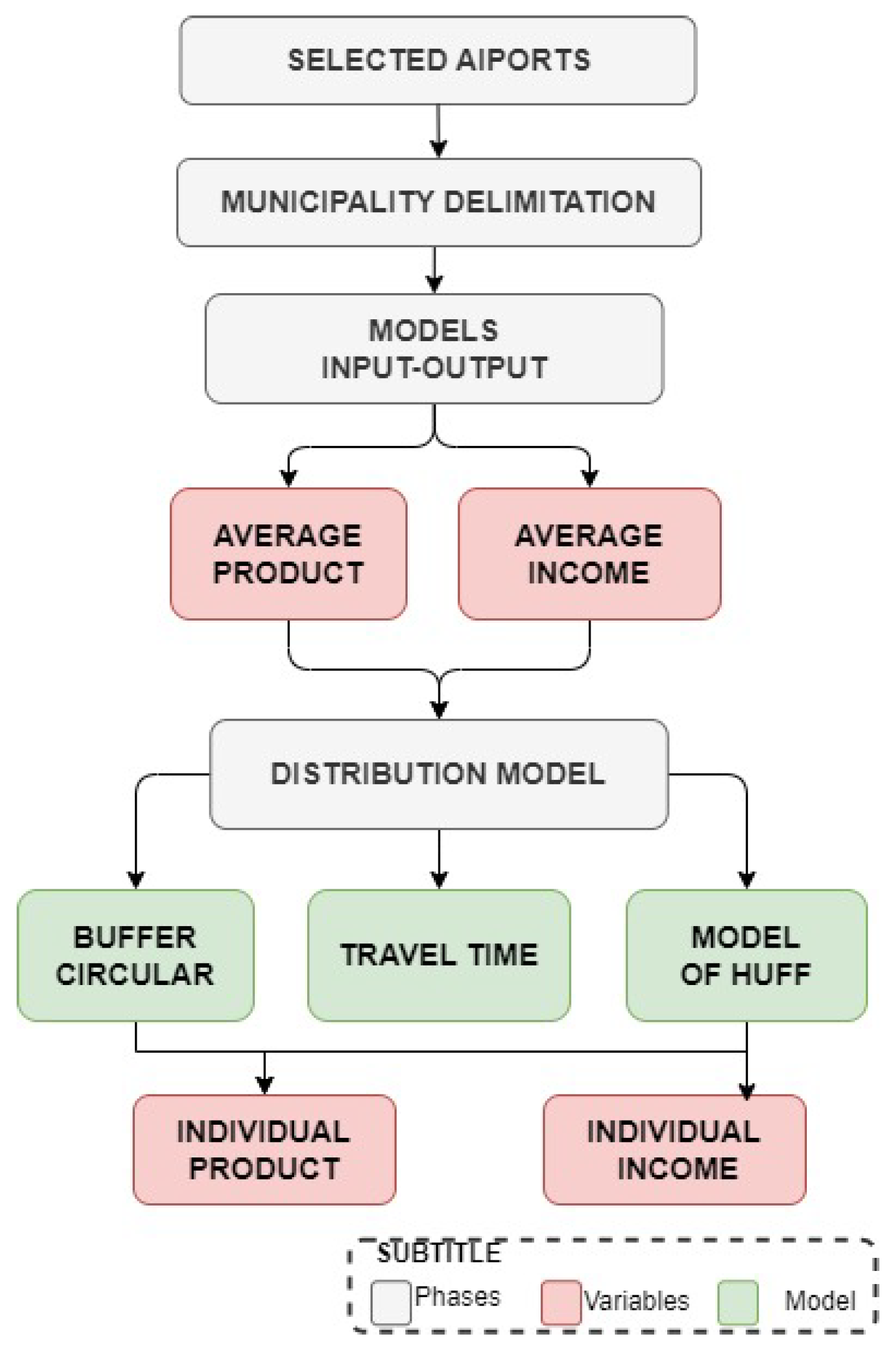
Figure 2.
Movement of Passengers and Air Cargo Airport SBSP, SBGR, and SBKP. Source: ANAC [22].
Figure 2.
Movement of Passengers and Air Cargo Airport SBSP, SBGR, and SBKP. Source: ANAC [22].

Figure 3.
Area of influence of airports.

Figure 4.
Product variables for SBSP, SBKP, and SBGR airports using the circular buffer model.
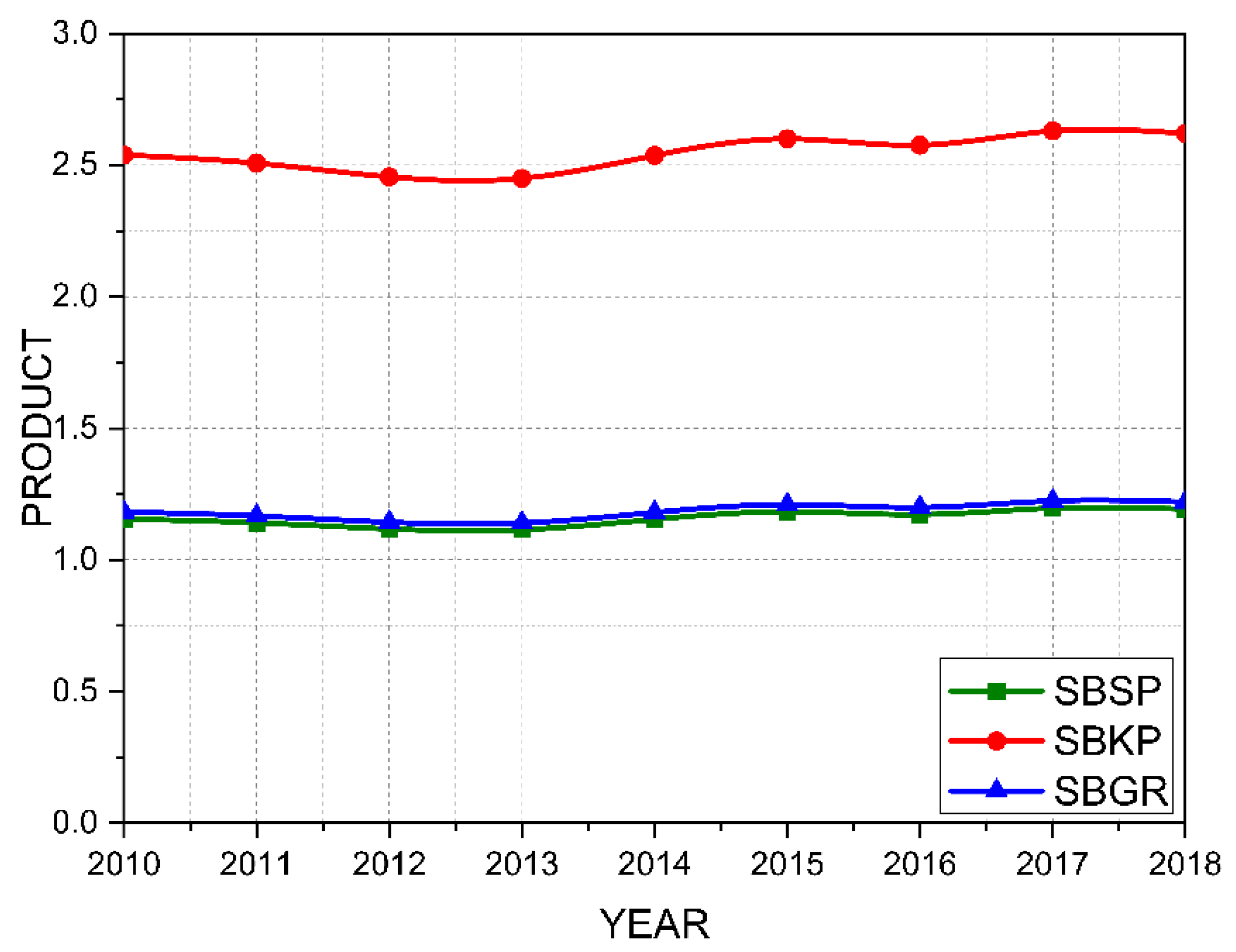
Figure 5.
Product variable for SBSP, SBKP, and SBGR airports using the travel time model.
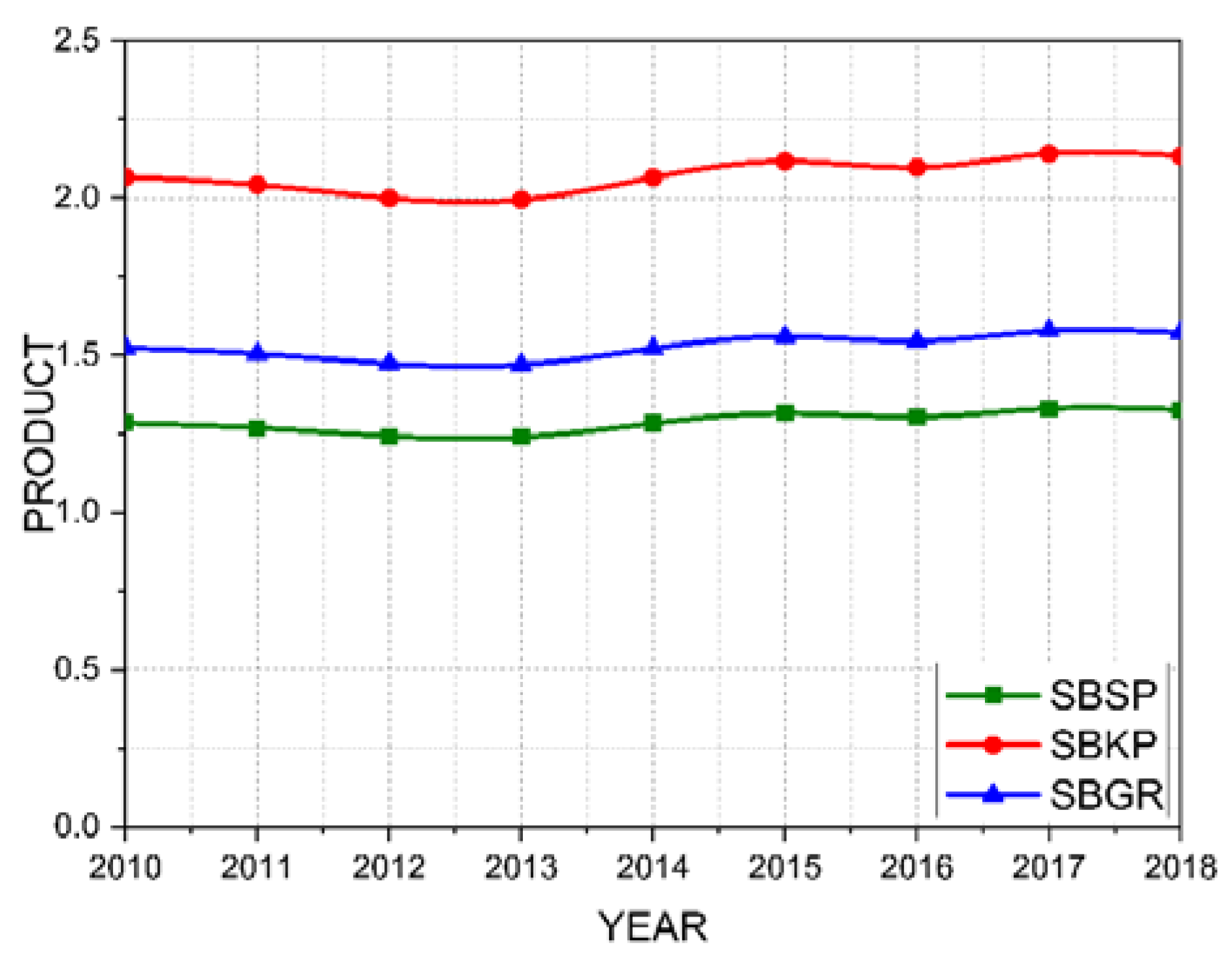
Figure 6.
Product variables for SBSP, SBKP, and SBGR airports using the Huff model.
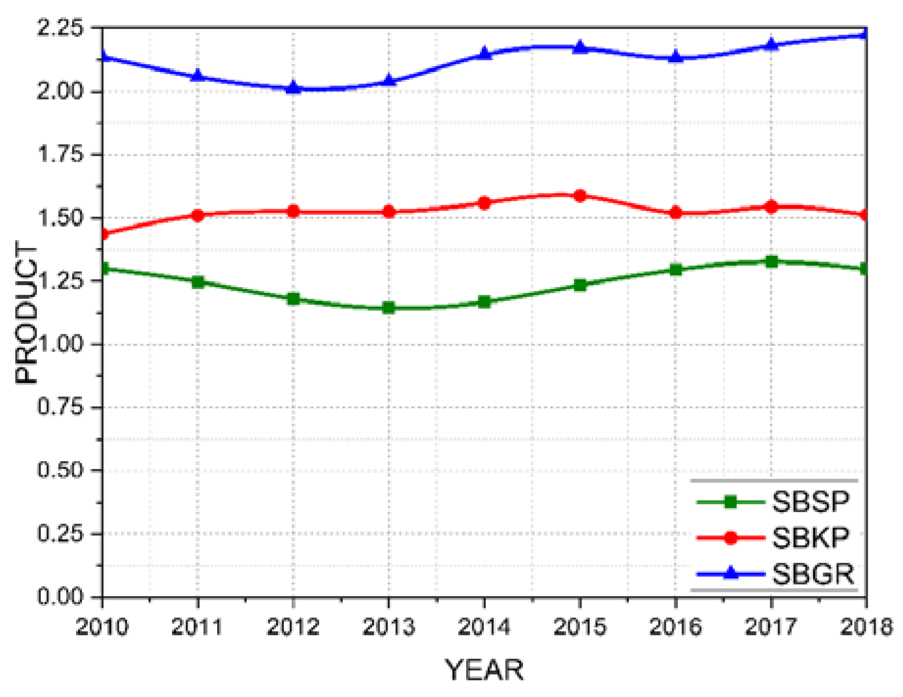
Figure 7.
Income variable for SBSP, SBKP, and SBGR airports using the circular buffer model.
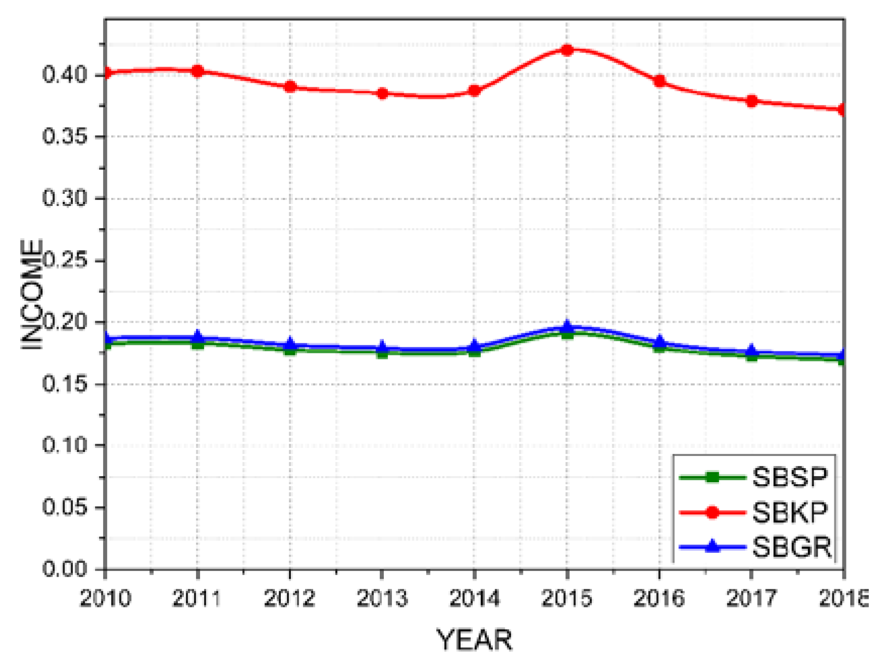
Figure 8.
Income variable for SBSP, SBKP, and SBGR airports using the travel time model.
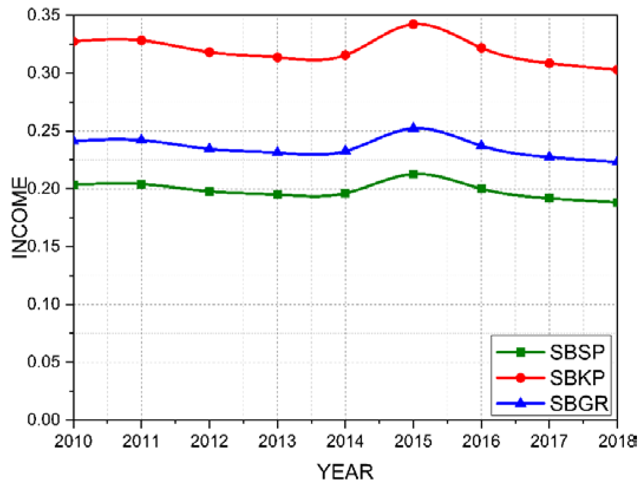
Figure 9.
Income variable for SBSP, SBKP, and SBGR airports using the Huff model.
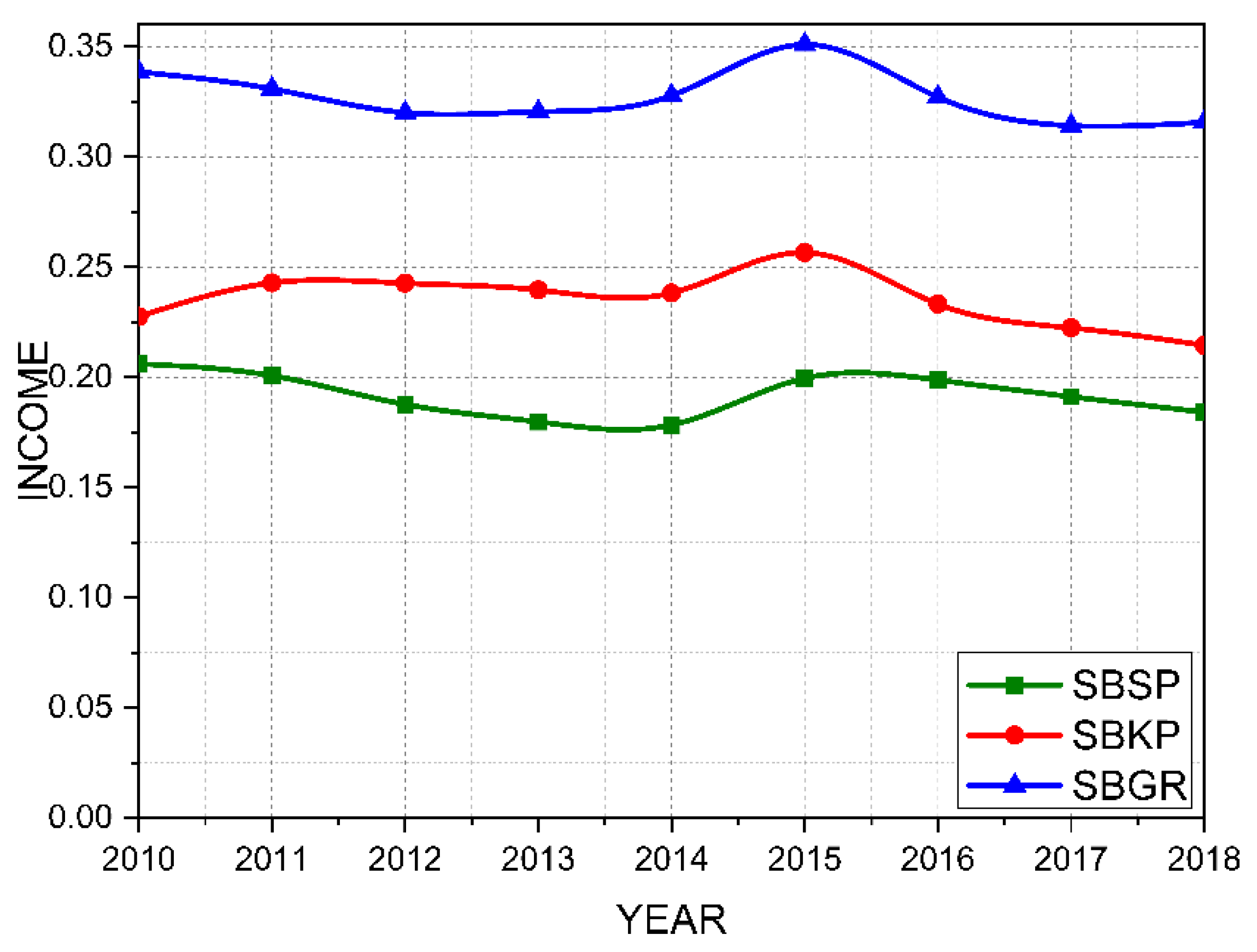

Table 1.
Systematic Reviews on the input-output model and economic growth.
| AUTHOR/YEAR | DATA | MODELS | DESCRIPTIONS |
|---|---|---|---|
| Tveter [6] | - Population size - Jobs. |
Difference in difference model. | The author studied the impact on population growth due to regional airports. |
| Nasution et al. [5] | GDP – Gross Domestic Product. -Movement of passengers. -Cargo handling |
Input-Output Vector Error Correction Method. |
The article shows a relationship between air transport and economic growth in Indonesia. Relating data on passenger/air cargo movement and GDP. |
| Yu [7] | -Economic impact models. - Econometric models. |
Input-Output CGE - Equilibrium General Computable. |
The article describes IO modeling and IO model applications. Economic modeling includes single regions and multi-region. |
| Aden [8] | - GDP – Gross Domestic Product. - Passenger movement (domestic and international. - Product and Mobilities (2016). - Pearson correlation analysis. |
Growth model based on GDP and passenger movement. |
The authors correlate economic growth and the contributions of air transport. And they point out two critical factors for development: Tourism and transport logistics. |
| Bagoulla e Guillotreau [9] | - Employment-inducing effects. -Environmental effects. |
Circular buffer model, travel time, Thiessen polygons, and Huff. | Maritime transport in France. Using Input-Output to measure the effects of production and induced jobs. |
| Subanti et al. [10] | - Indonesia air transport matrix data. | Inter-regional input-output model. | The article identified which sectors of the Indonesian economy have the most interregional effects. |
| Bandeira et al. [11] | - Brazilian IO tables from IBGE. | Input-Output | The authors presented an input-output model to analyze the metropolitan region of Campinas, São Paulo, Brazil. |
| Keček et al. [12] | - Production. - Product aggregates. - Job multipliers. |
Input-Output | The article shows a macroeconomic analysis. The results show that the air, land, and maritime transport sectors have a significant growth in the job multiplier. |
| Mishra et al.[13] | - GDP – Gross Domestic Product. | Pedroni’s method Ordinary squares model Vector Error Correction Method. |
The paper presents a study of 15 states in India to assess economic links with air traffic. |
Table 2.
Attractiveness coefficient according to the travel time model for SBSP, SBGR, and SBKP airports.
Table 2.
Attractiveness coefficient according to the travel time model for SBSP, SBGR, and SBKP airports.
| AIRPORT | SBSP | SBGR | SBKP |
|---|---|---|---|
| T(P, A) | 0.264 | 0.312 | 0.424 |
Table 3.
Attractiveness coefficient according to the circular buffer model for SBSP, SBGR, and SBKP airports.
Table 3.
Attractiveness coefficient according to the circular buffer model for SBSP, SBGR, and SBKP airports.
| AIRPORT | SBSP | SBGR | SBKP |
|---|---|---|---|
| D(P, A) | 0.237 | 0.242 | 0.521 |
Table 4.
Attractiveness coefficient according to the Huff model for SBSP, SBGR, and SBKP airports.
| Year | SBSP | SBGR | SBKP |
|---|---|---|---|
| 2010 | 0,287 | 0,266 | 0,446 |
| 2011 | 0,276 | 0,292 | 0,431 |
| 2012 | 0,265 | 0,304 | 0,431 |
| 2013 | 0,257 | 0,307 | 0,436 |
| 2014 | 0,252 | 0,306 | 0,442 |
| 2015 | 0,259 | 0,306 | 0,435 |
| 2016 | 0,274 | 0,296 | 0,430 |
| 2017 | 0,277 | 0,291 | 0,432 |
| 2018 | 0,273 | 0,282 | 0,445 |
Table 5.
Average updated product for São Paulo airports.
| AIRPORT | AVERAGE | STANDARD | MARGIN OF ERROR |
|---|---|---|---|
| DEVIATION | (~95% I.C.) | ||
| SBSP | 12,435 | 0,0670 | 0,0438 |
| SBKP | 15,241 | 0,0270 | 0,0270 |
| SBGR | 21,218 | 0,0466 | 0,0466 |
Table 6.
Updated average income for São Paulo airports.
| AIRPORT | AVERAGE | STANDARD | MARGIN OF ERROR |
|---|---|---|---|
| DEVIATION | (~95% I.C.) | ||
| SBSP | 0,1918 | 0,0100 | 0,3273 |
| SBKP | 0,2353 | 0,0123 | 0,0117 |
| SBGR | 0,3273 | 0,0082 | 0,0077 |
Disclaimer/Publisher’s Note: The statements, opinions and data contained in all publications are solely those of the individual author(s) and contributor(s) and not of MDPI and/or the editor(s). MDPI and/or the editor(s) disclaim responsibility for any injury to people or property resulting from any ideas, methods, instructions or products referred to in the content. |
© 2024 by the authors. Licensee MDPI, Basel, Switzerland. This article is an open access article distributed under the terms and conditions of the Creative Commons Attribution (CC BY) license (https://creativecommons.org/licenses/by/4.0/).
Copyright: This open access article is published under a Creative Commons CC BY 4.0 license, which permit the free download, distribution, and reuse, provided that the author and preprint are cited in any reuse.


