1. Introduction
The classification of sediments on the seafloor is a crucial aspect of ocean exploration, and is essential for the development of marine resources, construction of marine engineering, and maintenance of the marine ecological environment. The use of acoustic data for seafloor sediment classification is in line with the modern concept of sustainable development, and is more automated and intelligent than the conventional mechanical sediment sampling method. This method has a vast research scope and application prospects. Several studies have been conducted on seabed sediment classification based on multibeam backscatter intensity and side-scan sonar data. In 1999, Hamilton et al. conducted a comparative study on the classification performance of RoxAnn and QTC-View classification software[
1]. Preston et al. investigated the correlation between relevant parameters of submarine rock and soil and acoustic substrate[
2]. In 2000, Tegowski analyzed the fractal characteristics of echo signals[
3]. In 2001, Preston obtained backscattering data of seafloor sediments from shallow sea areas, performed principal component analysis on nearly 130 characteristic quantities, and selected the optimal features for sediment classification to identify fine sediment types on the seafloor[
4,
5]. In 2010, Giovanni et al. explored the relationship between sounding data, scattering intensity data, and the angular response of scattering intensity and sediment granularity, distribution of seafloor grasses, and relative scattering intensity threshold of five types of sediments, including gravel, gravel sand, and argillaceous sand with a small amount of gravel[
6]. In 2013, Wienberg et al. utilized multi-beam sonar technology to scan the submarine coral mountain between the Iberian Peninsula and Madeira Islands in the northeast of the Western Pacific Ocean and classify the sediments[
7]. Currently, multi-beam backscattering intensity data is the primary method for seafloor sediment classification. This method is effective in classifying gravel, sand, clay, and other types, but it faces challenges in achieving ideal results when the sediment differences are small.
Sub-bottom profiling is a widely used technique for exploring submarine stratigraphy based on acoustic principles. The geological interpretation of sub-bottom profiles is based on the echo characteristics and morphology. This technique is commonly used in preliminary geological investigations for offshore wind power site surveys, submarine routing pipeline laying, and other offshore engineering constructions due to its high detection resolution, fast and convenient nature, and low cost [
8,
9,
10,
11]. However, conventional engineering geological exploration processes the sub-bottom profiling data in a simple manner, resulting in low data utilization, low interpretation accuracy and precision, and other issues[
12,
13]. Recently, the inversion of seafloor sediment properties using sub-bottom profile data has emerged as a new way of implementing sub-bottom profiling data for sediment classification. Chirp sub-bottom profiler data have been successfully used to quantify the physical property parameters of shallow sediments on the seafloor. Statistical analysis of chirp profiles and sediment test data has been used to analyze the distribution patterns and deposition processes of surface sediments and sedimentation processes[
14]. Inversion of the velocity, particle size, sediment type, and other properties of surface sediments has been achieved using chirp sonar data[
15,
16]. The parameters obtained were highly consistent with laboratory findings. Genetic algorithms have been applied to sub-bottom profiling to obtain impedance profiles, successively obtaining engineering geological parameters based on the empirical relationship between wave impedance and sediment mechanical properties[
17].
In recent years, Convolutional Neural Networks (CNN) based on deep learning methods have been extensively used in various fields such as object detection, face recognition, and text classification [
18,
19,
20]. It has become a research trend to apply CNN methods for the inversion of seafloor physical property parameters and sediment classification. Berthold et al. used GoogLeNet to preliminarily classify gravel, mud, sand, and mixed sediment[
21]. Luo et al. compared the classification performance of deep and shallow CNN models for three types of sediment, namely stone, mud, and sand, and found that the shallow CNN model outperformed the deep CNN model while achieving excellent classification performance[
22]. Wang et al. conducted a study on sediment classification using MSC-Transformer and shallow formation profile data, and achieved good results[
23]. Additionally, Lu Liang et al. used texture features and the K-means clustering algorithm to classify seafloor sediments and determine the optimal number of classifications[
24].
This paper proposes an automatic classification method for seafloor sediment types in the Northern Slope of the South China Sea using an improved U-Net and K-means clustering algorithm. The method utilizes multi-beam depth, topographic slope, reflection intensity of the sub-bottom profile, and sample test data to predict the average particle size of the seafloor. The U-Net network model with low dimensional feature retention and pooled index sampling is established to achieve this prediction. The optimized K-means clustering algorithm is then used to classify sediment types. In the initial clustering center selection stage, the edge extraction effect of sediment types is optimized by comparing the error squares and searching the density center as the initial clustering center, which improves the classification accuracy of seafloor sediment types. The classification results are analyzed comprehensively with the geological background and sediment distribution characteristics of the study area to further divide the sedimentary environment of the study area and explore the distribution rule and sedimentary characteristics of the study area. This provides data support for the understanding and understanding of the sedimentary environment and sedimentary process of the Northern Slope of the South China Sea and has important practical significance for the development of nearby resources.
2. Study area overview and Data
The Northern Slope region of the South China Sea is a complex topographical area with a series of submarine canyons [
25,
26] and a water depth ranging from 400 m to 2500 m. There are two types of seafloor surface sediments in this area[
27]: modern fine-grained debris transported by rivers and early late Pleistocene glacial low sea level residual deposits. The sediment particle components exhibit interleaved deposition of coarse and fine grains, with coarse-grained materials having a high content due to long-term deposition in high-energy environments. These materials may be covered by fine-grained sediments during the post-glacial sea level rise[
28], influenced by the characteristics of the sediments in the provenance area and their later transformation. The seafloor sediments in the Northern Slope of the South China Sea exhibit distinct zonal distribution characteristics[
29]. The shallow water area sediments are mainly silty clay and silty sand, while the deep water area sediments with water depth greater than 1000m are mainly fine-grained clay and silty clay[
30].
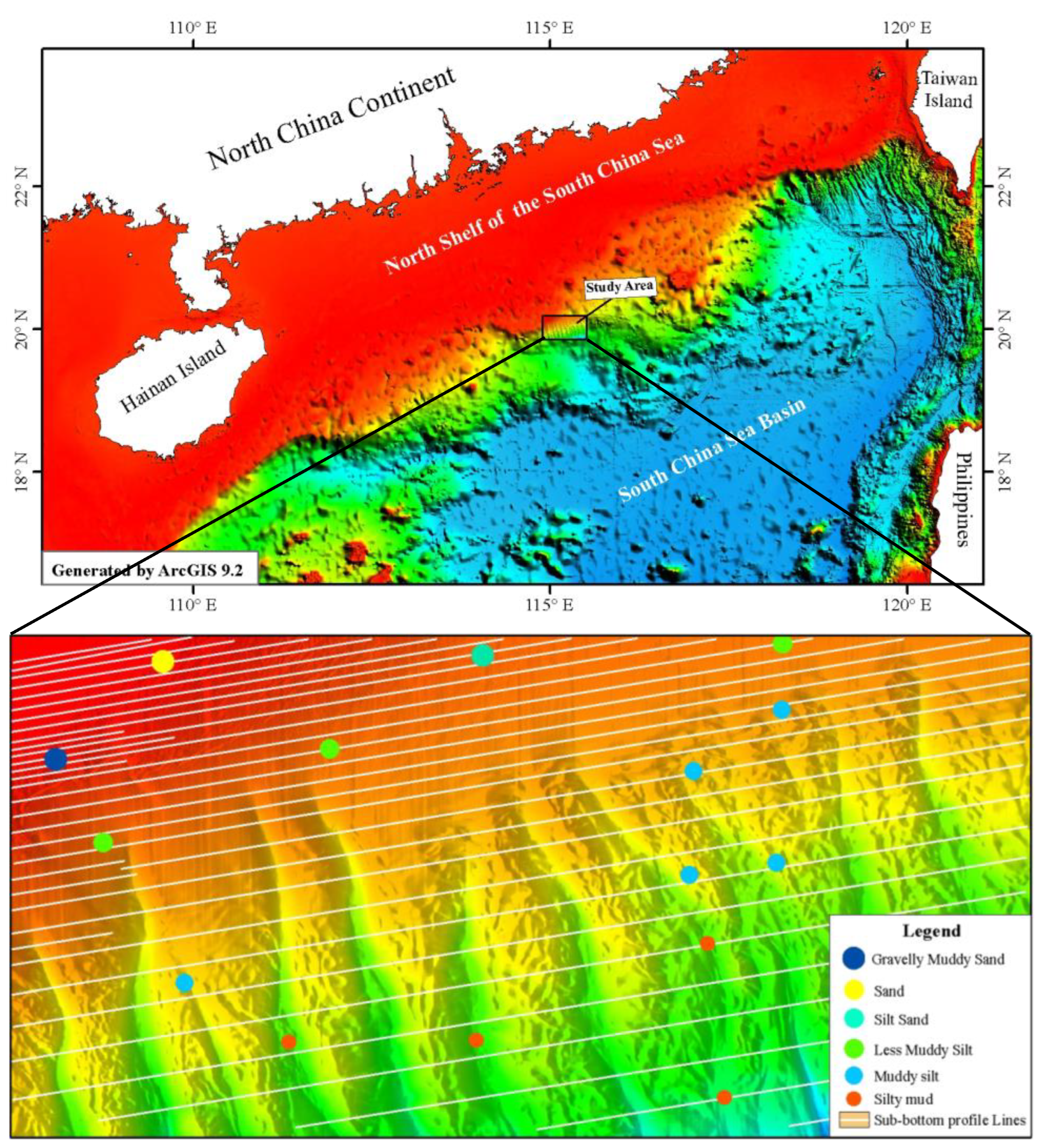
Figure 1 depicts the spatial distribution of the research area, sub-bottom profile lines, and sampling stations. The research area is covered by 36 sub-bottom profile lines, with a minimum line spacing of 400m and a maximum of 2000m. The sampling stations are sparsely distributed throughout the region, totaling 15. Based on the analysis of the collected data, the seafloor sediment types in the study area can be classified into six types: gravelly muddy sand, sand, silty sand, less muddy silt, muddy silt, and silty mud.
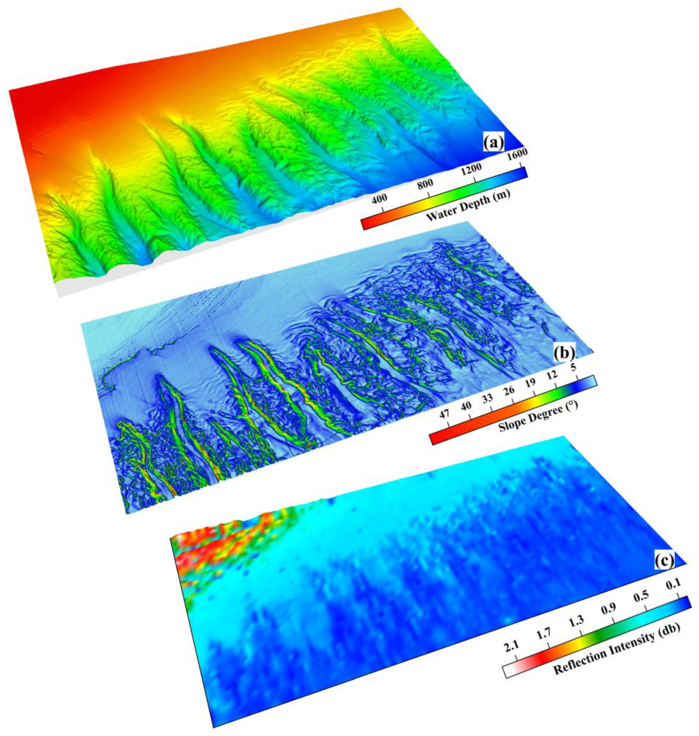
The present study utilizes a dataset comprising of multi-beam depth, topographic slope, seafloor reflection intensity of the sub-bottom profile, and mean grain size data obtained from sampling tests in the study area. The multi-beam water depth data is processed using Caris HIPS 11.4 software. The processed data undergoes tide correction, draft correction, sound velocity correction, and error correction, followed by merging and coordinate conversion. A DTM data grid of 20 m * 20 m is then constructed. The water depth data and terrain slope data are output after editing and processing. The sub-bottom profile data is processed using the TRITON SB-Interpreter developed by TRITON IMAGINE Company. The processing includes channel head processing, bandpass filtering processing, amplitude gain, etc. The sea bottom reflection intensity value is extracted based on the processed shallow formation section data. Kriging interpolation is employed to generate regional seafloor reflection intensity data. The spatial distribution characteristics of water depth, slope, and seafloor reflection intensity in the study area are presented in
Figure 2.
3. Method
3.1. Improved U-Net
The U-Net network, originally proposed by Ronneberger et al.[
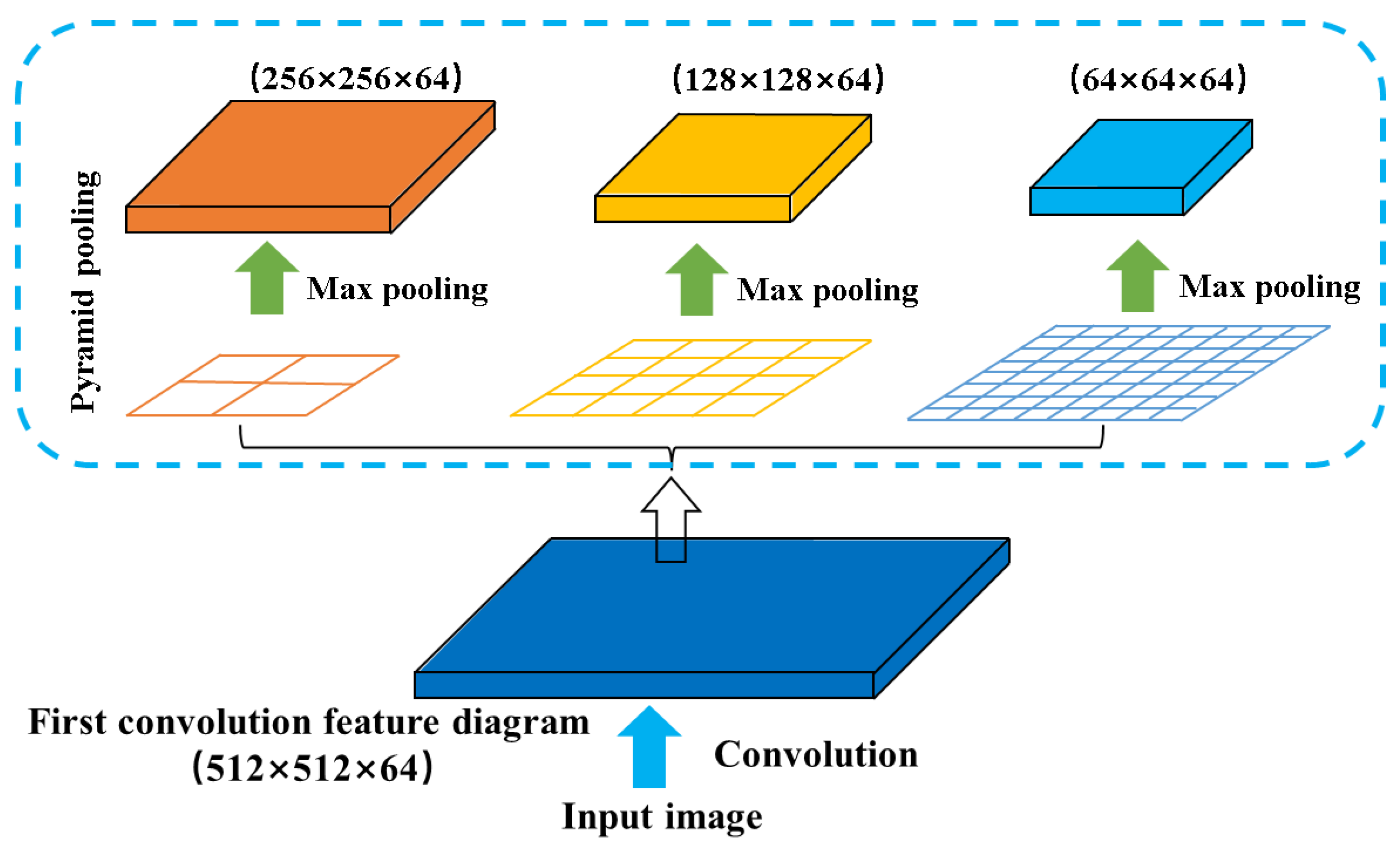
31] in 2015, has been successfully applied to the semantic segmentation of medical images. However, the construction of relationships between physical property parameters of submarine sediments is more complex than that of cell organs in medical images. The U-Net network architecture consists of an encoder and a decoder with encoder symmetry structure. The encoder is responsible for obtaining semantic information, while the decoder performs the process of downsampling and upsampling of data. The decoder uses a typical convolutional network structure, which alternates between multi-layer convolution and pooling operations to gradually reduce the resolution of feature data and double the number of channels of feature data at each layer. To obtain global information about the data, each step in the decoder corresponds to the encoder, including the upsampling of the feature data followed by multiple convolution. The decoder gradually improves the resolution of the output feature data while reducing the number of channels of the feature data by half. To locate the upsampled features, the decoder splices them with feature data of the same resolution from the decoder via skip connections. However, with the deepening of the network, low-dimensional details of the input data are weakened after multiple convolution operations, and the computational effect of the edge contour of the data volume cannot be guaranteed. To address this issue, the spatial pyramid pool layer is introduced into the coding part of the network to preserve low-level features. The pyramid pooling layer reduces the low-dimensional feature data volume of the first convolution layer of U-Net to 1/2, 1/4, and 1/8 of the original size, and then performs feature fusion with the corresponding scale levels through dimension superposition.
Pooling is a crucial process for extracting features from data. It enables the optimal utilization of data information and storage resources by eliminating redundant information and preserving essential information. This, in turn, reduces the number of calculation parameters while ensuring accuracy. The pyramid pooling technique is based on multi-scale pooling, as illustrated in
Figure 3. At the top of the pyramid, global averaging pooling is employed to extract the global context characteristics of the input.Initially, the input data is fed into a convolutional layer, resulting in a low-dimensional feature data body of size 512×512×64. Subsequently, maximum pooling is performed with pooling window sizes of 2×2, 4×4, and 8×8. The proposed method involves the utilization of global average pooling to extract local features of varying sizes within sub-regions. Subsequently, a 1x1 convolution is employed to reduce the dimensionality of the extracted features, thereby minimizing computational requirements. Finally, the pooling outcomes of different sizes are up-sampled to match the dimensions of the input feature graph, and the channel superposition fusion is performed to generate the ultimate output of the pyramid pooling module. The resulting low-dimensional feature data is then pyramided, resulting in feature data of sizes 256×256×64, 128×128×64, and 64×64×64. To ensure that each coding layer contains both detailed information of low-dimensional features and abstract high-dimensional features, the low-dimensional feature data of different scales are fused with the features of each level of the corresponding coding layer through dimensional superposition. This approach enables the establishment of a more accurate relationship between the physical property parameters of seafloor sediment.
To enhance the extraction of seafloor sediment type edges, a pooled index upsampling technique is employed in the decoding layer. Initially, the encoder conducts convolution and max pooling operations, where the position of the corresponding max pooling index is stored. Subsequently, the decoder performs upsampling and convolution, and each pixel is sent to the classifier. During the upsampling process, the corresponding max pooling index from the encoder layer is retrieved to perform upsampling. In comparison to the conventional U-Net's deconvolution upsampling method, the pooled index upsampling technique sharpens the image edges, obviating the need for learning upsampling and reducing the network training parameters.
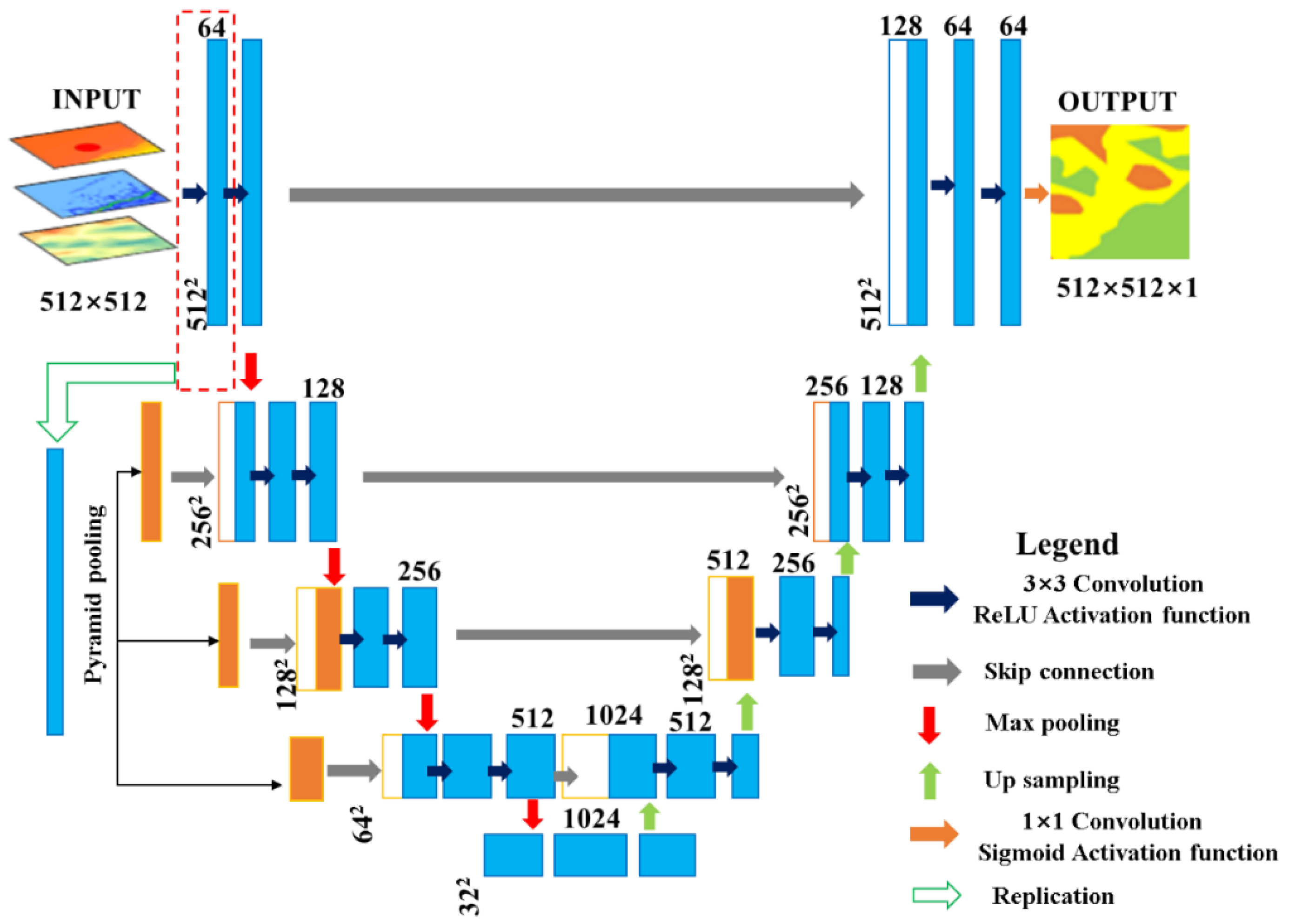
The improved U-Net architecture is depicted in
Figure 4, which utilizes the U-shaped symmetrical structure of the standard U-Net. The network is composed of three parts, namely, downsampling, upsampling, and a skip connection structure. The encoder, located on the left side of
Figure 4, performs compression by reducing the image size and extracting the feature map using two repeated convolution layers and one pooling layer. The convolution layer in the compression path (encoding layer) has a convolution kernel size of 3 × 3, and the rectified linear unit function is used as the activation function in the network. After the first convolution, the image retains low-level features through spatial pyramid pooling operation. The feature map obtained from the first convolution layer (conv1_1) is reduced to 1/2, 1/4, and 1/8 of the original size and then fused with pool1_3, pool2_4, and pool3_4, respectively. The pooling operation of the network combines max pooling and record indexing. In the decoder, located on the right side of
Figure 4, the size of the last convolutional kernel in each decoding layer is halved to ensure that the feature map during upsampling has the same number of dimensions as the one after pooling in the encoding layer. Nonlinear upsampling of the feature map is then performed with the pooling index, as described by Vijay et al.[
32].
3.2. Optimized K-means clustering algorithm
The K-means algorithm is a widely used clustering algorithm in the field of data mining and knowledge discovery[
33]. It is based on partition and is known for its simplicity of thought and fast convergence speed. The algorithm is an iteration-based repartition strategy that divides a given dataset into K cluster classes. During the iterative process, the Euclidean distance between each data point and the clustering center is optimized. The data point set X = {
x1,…,
xN} is partitioned into K clusters {
C1,…,
CK}represented by K partition centers
. The objective function of the algorithm can be expressed as follows:
The K-means algorithm is a clustering method that aims to minimize a given objective function. The algorithm iteratively seeks the minimum value of the objective function. The basic K-means algorithm involves three steps:
1. Initialization: The algorithm starts by dividing all samples into K initial clusters.
2. Classification: Each sample in the dataset is assigned to the cluster with the closest center (mean). The distance between samples is typically calculated using Euclidean distance, either with standardized or non-standardized data. After classification, the centers of the clusters are recalculated based on the samples assigned to each cluster.
3. Iteration: Steps 2 is repeated until no further sample can be reassigned to a different cluster.
It is worth noting that step 1 can also begin with a specified set of K initial centers, rather than dividing the samples into K initial clusters.
The traditional K-means algorithm generates initial clustering centers randomly, which can result in unstable clustering outcomes, causing the same dataset to produce different clustering results. This algorithm is highly sensitive to the initial clustering center, as the N clustering centers randomly selected in the early stage of the algorithm may be isolated points or several points of the same class. The quality of clustering results is affected if the initial clustering center is not selected appropriately. The objective function J of the K-means algorithm calculates the sum of squares of minimized errors, and its formula is as follows:
Here, k represents the total number of subsets divided, Ok is the clustering center of the KTH cluster, and d(xi, Ok) represents the distance between the data sample of the KTH cluster and the clustering center. The calculated sum of squares of error can only reach the minimum when the selected clustering center is located in the density center of the data set. Therefore, this paper proposes an optimized K-means clustering algorithm based on this principle. In the initial clustering center selection stage, the point at the density center is found as the initial clustering center by comparing the sum of squares of error, which solves the sensitivity of the initial clustering center of K-means. During the clustering process, the same area projection method is used to project the structural plane onto the unit circle plane, and the Euclidean distance of two-dimensional points is used as the similarity measure of the structural plane. The optimization algorithm has the advantages of easy programming, few iteration times, stable clustering results, and so on. It has a good effect when applied to the classification of seafloor sediment.
The following is a detailed description of the method:
1. For each data sample in the dataset, consider it as a potential clustering center and calculate its corresponding sum of squared errors. Select the data vector with the smallest sum of squared errors as the first initial clustering center.
2. Based on the existing clustering centers, calculate the average sum of squared errors (
) for the current dataset.
3. To select the next initial clustering center, calculate the sum of squared errors that can be reduced when each data sample is considered as a potential clustering center. For a data sample (x
i, y
i) as a potential clustering center, the expression is:
Only when
deJ>0, the sum of squared errors can be reduced. The sum of reduced errors is denoted as
sumdeJ.
Select the data sample with the maximum sumdeJ value as the next initial clustering center and add it to set U. Repeat step 2 until all clustering centers are found. When selecting a clustering center from the set D and adding it to U, the chosen center Xi should be removed from the data sample set D.
4. Classification of seafloor sediment
Figure 5 illustrates the classification process of seafloor sediment in the Northern Slope area of the South China Sea. Initially, the original multi-beam water depth and shallow formation profile data are processed to generate a dataset of seafloor depth, slope, and reflection intensity. Subsequently, the training set and the test set are obtained by matching positioning and image clipping of the sampled test data. The U-Net network structure is enhanced by incorporating a spatial pyramid pool layer in the coding part and utilizing the pool layer index sampling in the decoding part. The improved network model is trained, and the preliminary classification of the sediment type is performed. Finally, the K-means clustering analysis algorithm is employed to optimize the edge extraction effect of sediment type, leading to further classification results.
Utilizing processed data on water depth, slope, and reflection intensity of sub-bottom profiles, a training dataset was constructed in conjunction with sediment sampling data from the study area, as presented in
Table 1. This dataset encompasses six distinct types of seafloor sediment, including gravelly muddy sand, sand, silty sand, less muddy silt, muddy silt, and silty mud. The training data were utilized in the development of a network model, which established correlations between water depth, slope, reflection intensity, average particle size, and sediment type. This model was subsequently employed in the experiment of classifying seafloor sediment types.
5. Experimental Results
5.1. Improved U-Net classification
The improved U-Net model utilizes a fully supervised learning approach, which necessitates manual labeling of sample labels for seafloor sediment type in conjunction with sediment sampling data, as presented in
Table 1. To account for the enhanced computing capability and spatial characteristics of the U-Net network, the original training dataset is randomly trimmed to a size of 512×512 using the OpenCV open source library programming through Python language. Additionally, the following data augmentation techniques are applied to the dataset[
34]: (1) Rotation of the original data and corresponding label data by 90°, 180°, and 270°, respectively; (2) Mirroring of the original data and corresponding label data along the Y-axis; (3) Gaussian fuzzy operation on the original data; (4) Light adjustment to the original data; (5) Addition of Gaussian noise and salt and pepper noise to the original data. After the data augmentation process, the training dataset comprises 1440 512×512 data blocks. Furthermore, to reduce training costs and obtain robust results, the transfer learning strategy proposed by Kumar et al.[
35] is adopted in this study to fine-tune the existing network parameters, enabling the network to output high-level visual features that are robust and suitable for sediment type identification.
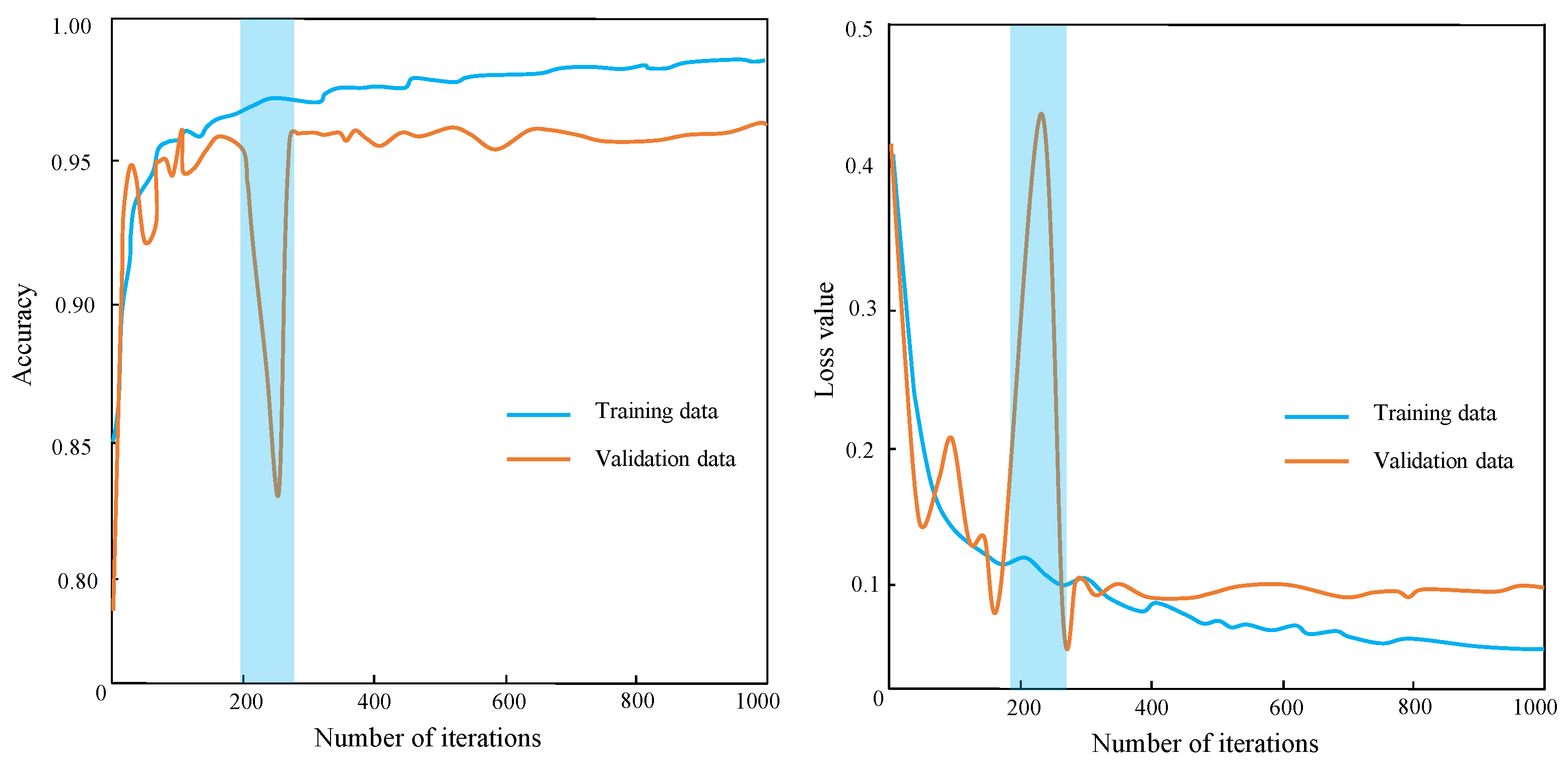
In this experiment, the batch size was set to 32, the epoch to 50, and the iteration times to 1000. The cross-entropy loss function was used as the objective function for the training network, with a learning rate of 0.1 and momentum of 0.9. The Stochastic Gradient Descent algorithm[
36] was employed to minimize the objective function and obtain the optimal model. The method of cross-checking was adopted to obtain the optimal test results for the parameters set in this paper[
37].
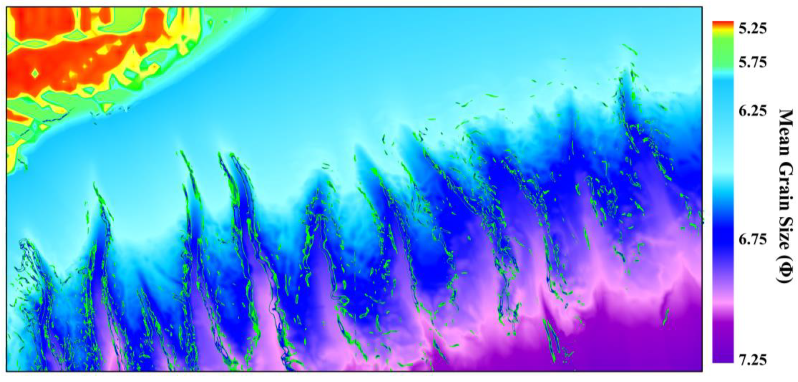
Figure 6 illustrates the changes in learning accuracy and loss value during the training process. The learning accuracy and loss value gradually decreased around 200 iterations, and the improved U-Net model gradually converged. Subsequently, the trained improved U-Net was used to classify sediment in the test datasets, with the range of each pixel within [0,1]. Finally, the prediction results were processed to obtain the mean grain size of the seafloor sediment, as shown in
Figure 7.
5.2. K-Means cluster analysis
The k-mean sediment classification method utilizes the cluster number K to classify seafloor sediment based on sampling results. This value represents a priori information and plays a crucial role in the accuracy of the classification. Selecting a value that is too small may result in the inability to differentiate between different types of seafloor sediments. Conversely, selecting a value that is too large may lead to inaccurate classification. To address this issue, this paper introduces two principles for determining an appropriate value for K in the classification of seafloor sediments.
(1) The Classification Principle of First-Class Groups in the Φ Standard Grain Size Classification Table
The Udden-Wentworth isometric grain size classification standard (hereinafter referred to as the "Φ Size Standard") is currently the most widely used grain size classification standard for sediments[
38]. The Φ particle size standard divides the seafloor into five types: rock, gravel, sand, silt, and clay. Based on these five types, the seafloor is further classified into subcategories, such as pebbled muddy sand, silty sand, muddy silt, silty mud, and so on. To determine the value of the classification number K, the number of class groups belonging to the seafloor sampling point type in the Φ standard classification table of particle size is first determined, and its value is set as the K value.
(2) The Principle of Regional Variation of Seafloor Sediment Type
The classification of seafloor sediment types based on the standard grain size classification table is a crucial step in understanding the characteristics of these sediments. However, it is important to consider the regional variation of seafloor sediment types and whether a finer classification can be carried out. This can be determined by assessing the value of K of the cluster type. The regional effect of the classification results of seafloor sediment is influenced by various factors, including seafloor sediment genesis and hydrodynamics. The type of seafloor sediment is expected to exhibit regional and continuous changes. Due to the correlation of these factors, there is often a certain degree of transition between seafloor sediment types. Increasing the value of K can improve the regional effect of multi-beam seafloor sediment classification results, indicating that the classification results are effective. Conversely, if the regional effect is not good, it suggests that the addition of classification is not appropriate. Therefore, it is important to consider the regional variation of seafloor sediment types when classifying them based on the standard grain size classification table.
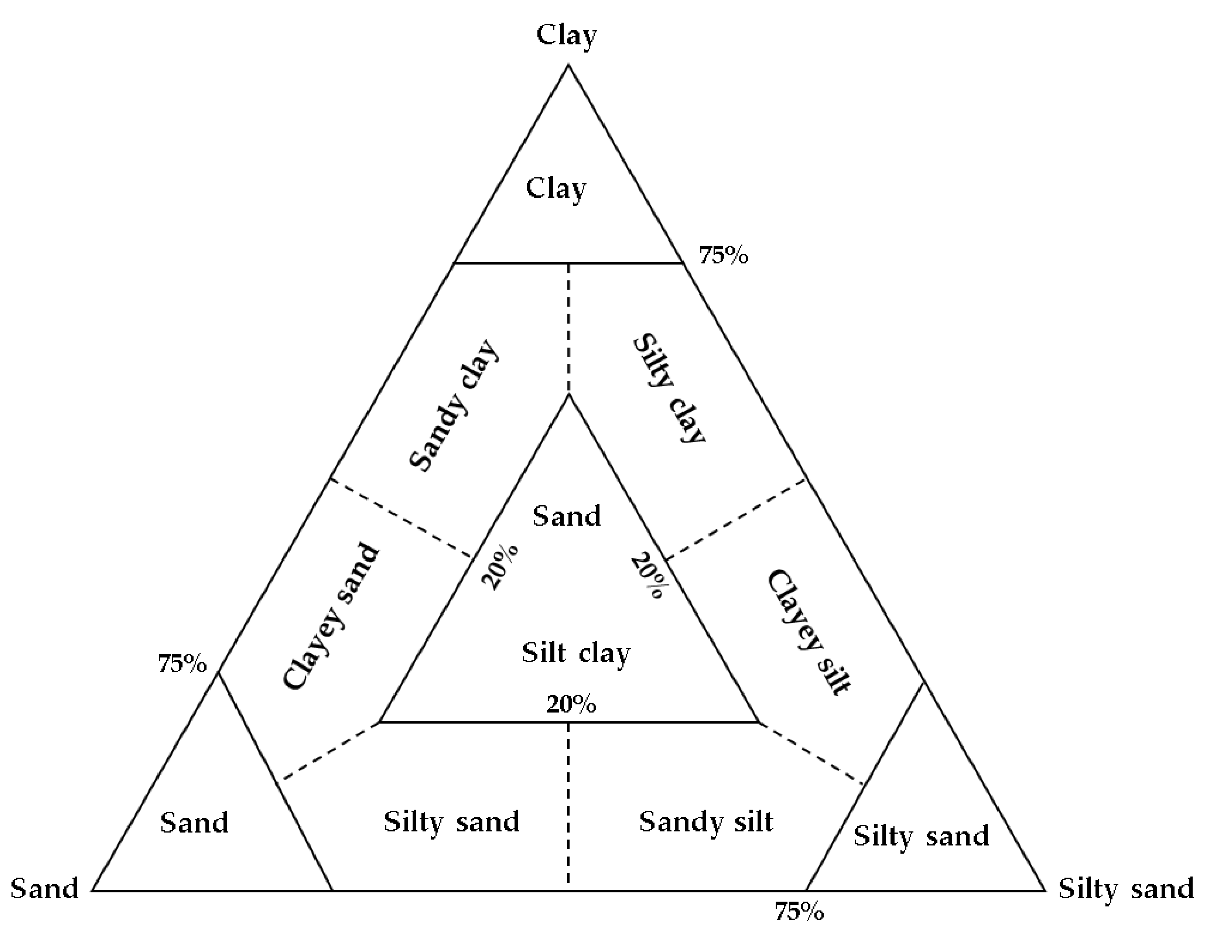
In the study area, the seafloor sediments can be classified into six types, namely gravelly muddy sand, sand, silty sand, less muddy silt, muddy silt, and silty mud. The classification of sediment types is based on Shepard's structural classification, which is widely used internationally. Shepard proposed this classification in 1954, which considers sand, silt, and clay as the three end-members of the triangular diagram and determines the grain size content as 20%, 75%, 40% to 75%, 12.5% to 50%, respectively[
39]. The classification of graveless sediments includes ten classes, as shown in
Figure 8.
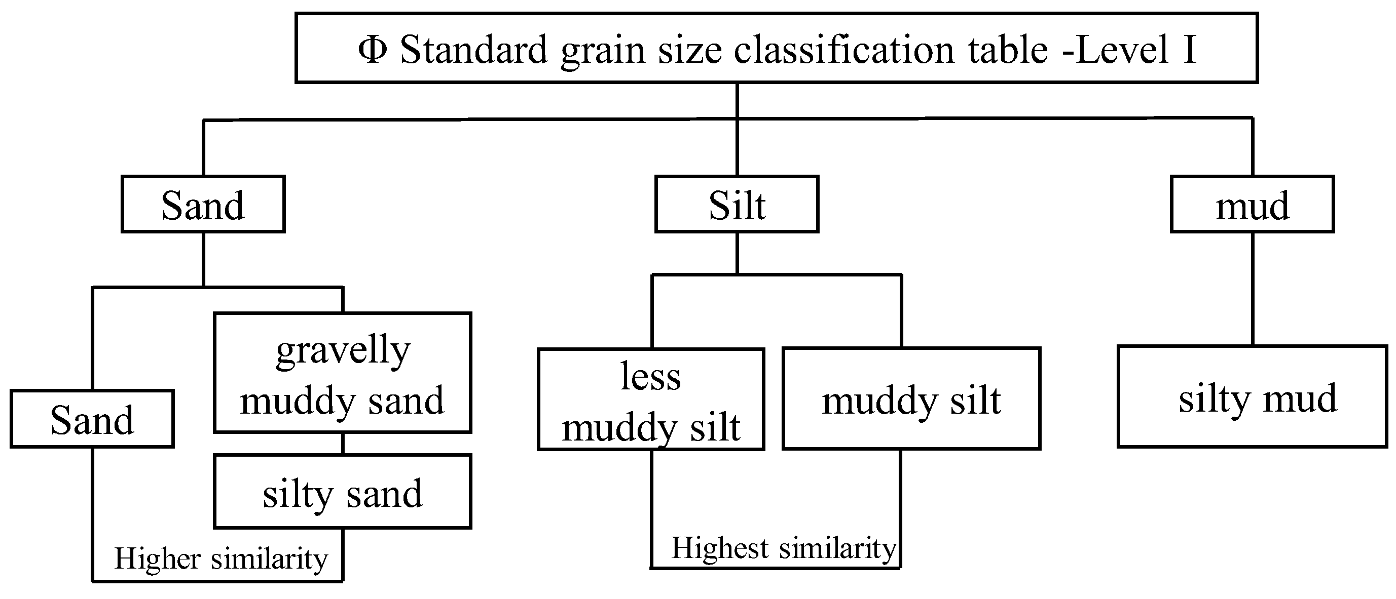
Applying the nomenclature principle and in conjunction with the Φ standard grain size classification chart[
40], we have depicted the schematic representation of the sediment subcategory in the surveyed region (refer to
Figure 9).
Based on the figure, it is evident that the sediment contains a relatively low amount of mud compared to less muddy silt and muddy silt, and the similarity between the latter two is remarkably high. Furthermore, the sediment contains a relatively low amount of silt compared to sand and silty sand, and the similarity between the two is the second highest. In the classification of seafloor sediment, the higher the similarity between sed-iment types, the more challenging it becomes to differentiate them. Analyzing the simi-larity of sediment types in the test area can aid in accurately selecting the classification of seafloor sediment and evaluating the ability of seafloor sediment classification. For instance, it can help determine whether sediment types with high similarity, such as sand and silty sand, can be automatically distinguished.
Cluster analysis is a method of grouping similar objects together while ensuring that different groups have the greatest dissimilarity. The process of cluster analysis relies on measuring the similarity between target data. In this study, the three-dimensional points of the unit normal vector of all structural planes were projected onto the projection plane using the equal area method. The similarity between two points (x
1, y
1) and (x
2, y
2) was measured using the Euclidean distance d, where a smaller distance indicates a higher degree of similarity between the structural planes. The formula for Euclidean distance is given by Equation (1):
When recalculating the clustering center of the data set, the arithmetic mean value of the three-dimensional points representing the structural plane cannot be used to represent the clustering center. However, when using the equal-area projection, all points are on the plane, so it is reasonable to use the arithmetic mean value when updating the sample center of the clustering process. The formula for calculating the sample center is given by Equation (2):
Here,
n represents the number of all sample sets in the
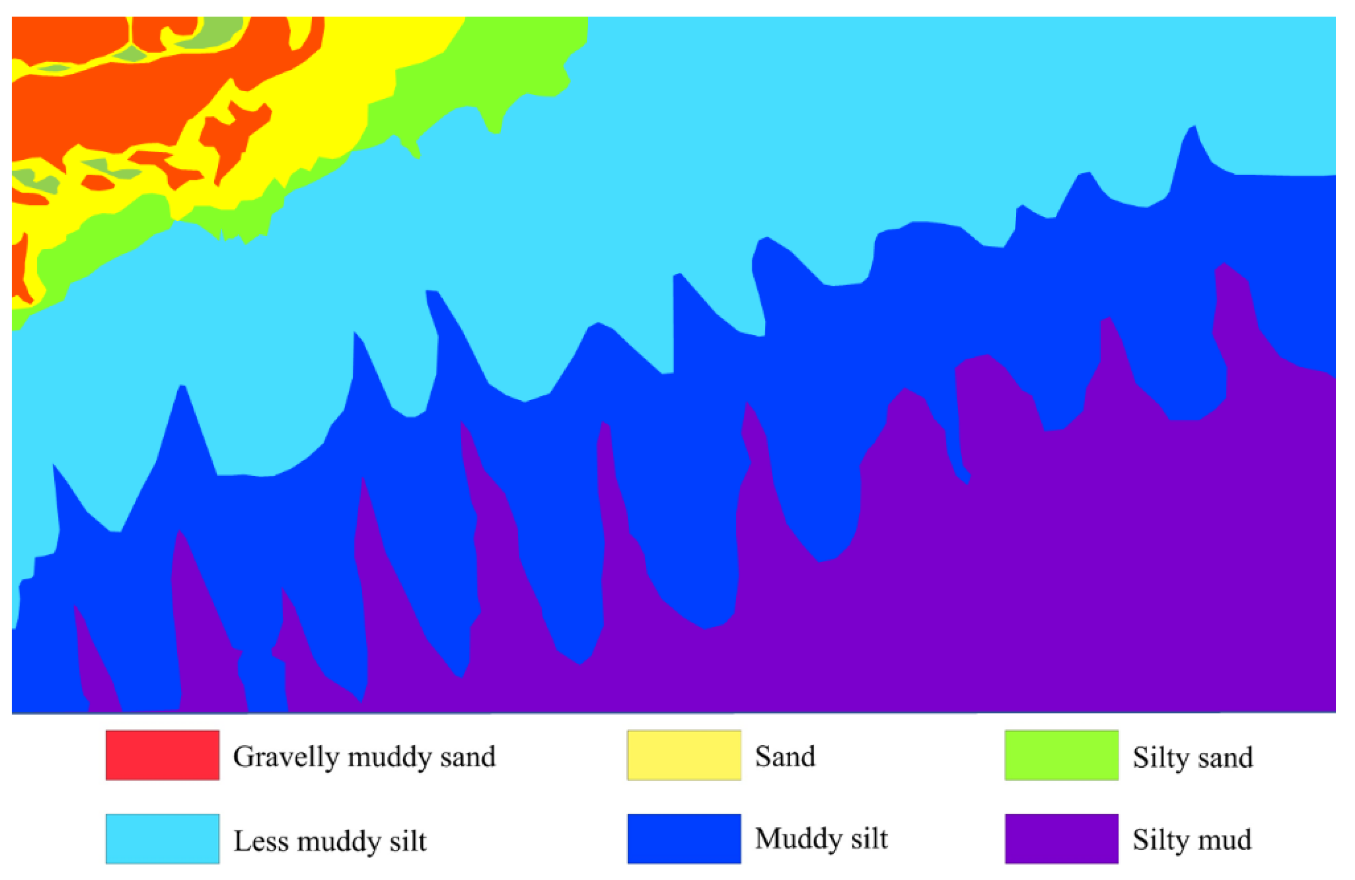
K cluster. Further K-Means clustering analysis was conducted on the classification results of the U-Net network to obtain classification results with a clear boundary of sediment type, as shown in
Figure 10.
6. Discussion and analysis
6.1. Benefits of Enhanced U-Net Method for Predicting Mean Grain Size
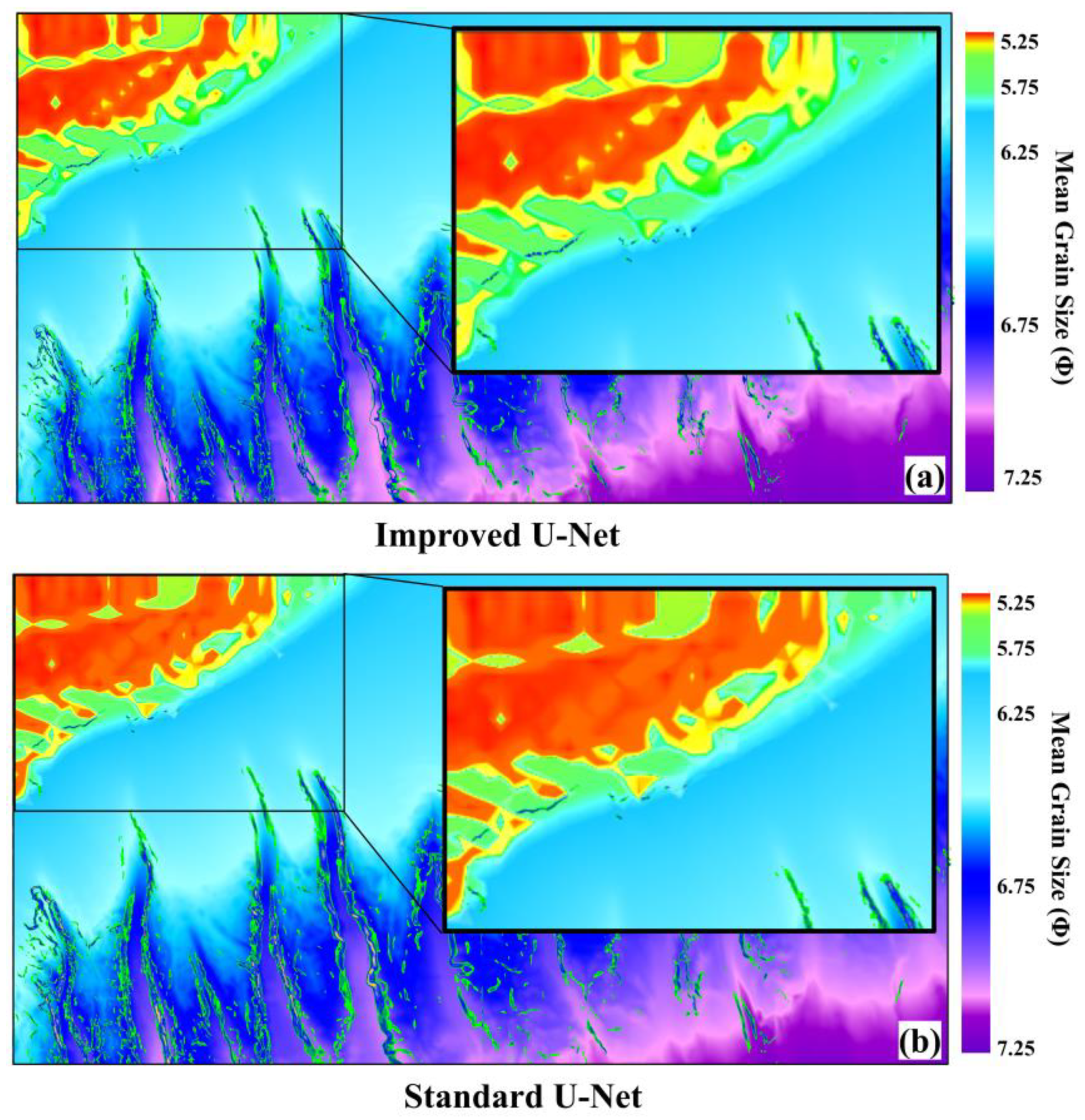
In this study, we compared the performance of the improved U-Net method for predicting average particle size with the standard U-Net network, while keeping the training and test sets constant. To evaluate the refining effect of the improved U-Net on the prediction results, we conducted a qualitative comparison by examining the local details of the results.
Figure 11 illustrates the comparison of the extraction results obtained from the two network models.
Upon comparison, it has been observed that the standard U-Net model gradually diminishes the low-dimensional features of the image. However, the improved U-Net model preserves the details of low-dimensional features at each coding layer and integrates them with the abstract information of the corresponding higher-dimensional features. This integration enhances the edge refinement effect of the base type, resulting in a more refined prediction output compared to the standard U-Net model.
To demonstrate the classification effectiveness of the improved U-Net and standard U-Net models, we have employed IoU and F1-Score metrics to evaluate the particle size prediction results of these two network models. IoU score is a widely accepted performance measure for object category segmentation, which represents the ratio of intersection and union between the truth set A and segmented result set B.
The F1-Score is a metric used to evaluate the effectiveness of image segmentation by taking into account both Precision and Recall[
42], namely:
Where, TP is the real value, i.e. A∩B; FP is true negative, namely B-(A∩B); FN is a false negative value, namely A-(A∩B).
The value range of
IoU and F1-Score is [0, 1]. The closer the result is to 1, the more accurate the prediction result of the mean particle size of the seafloor is. The quantitative evaluation of the prediction results of average particle size is shown in
Table 2.
The findings presented in
Table 2 demonstrate that the improved U-Net network yields superior average particle size prediction results. Specifically, the base classification results for the two indices increased by 4.9% and 2.8%, respectively, when compared to the standard U-Net network results. These results indicate that the improved U-Net model can enhance the accuracy of average particle size prediction in the study area.
6.2. Comparison of sediment classification results and sedimentary environment
The study area is situated in the outer margin of the ancient Pearl River Delta[
43]. The surface sediment is distributed in a NE-SW zonal direction parallel to the coast, with the grain size gradually decreasing with increasing water depth[
44]. The coastline has receded to the slope area with a depth of over 100m, leading to continuous erosion of the shelf slope break of the northern South China Sea and deposition of new terrigenous materials. The shelf and slope area have developed many buried ancient channels, coastal dunes, seafloor dunes, and underwater deltas[
45].
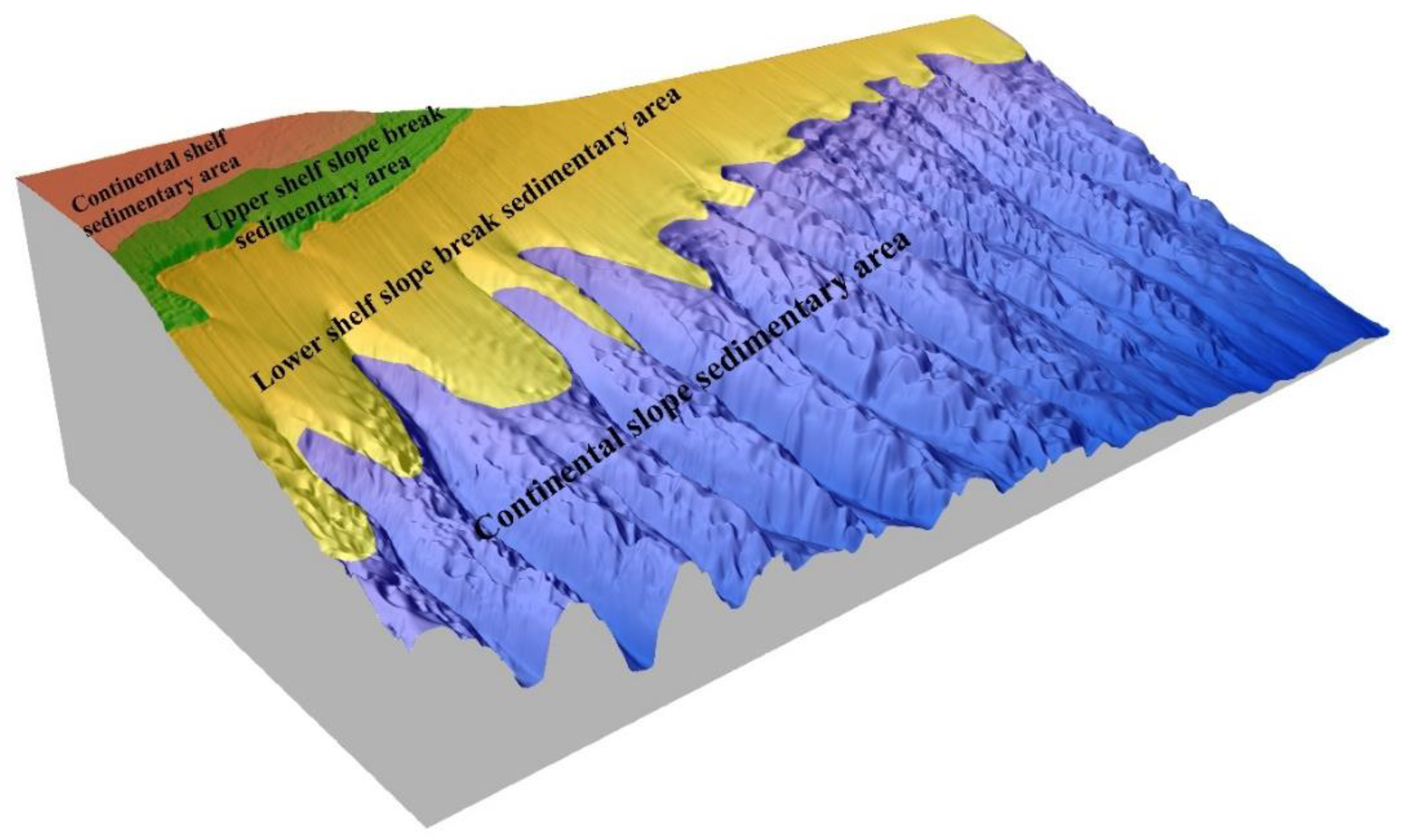
Based on the geological background and sediment classification, the study area was divided into four sedimentary environment zones, which are distributed in strips along the strike of the shelf slope break line, as shown in
Figure 12. Type I is the continental shelf sedimentary area, mainly distributed in the northwestern part of the study area, where the water depth is relatively shallow. The sediment is mainly pebbled sand and contains more gravel and ancient coral reef debris, with a relatively coarse average particle size. It is speculated that the beach sand or shallow sea sand has been screened by modern hydrodynamic conditions during the period of low sea level.
Type II is the upper shelf slope break sedimentary area, mainly located near the middle and upper shelf slope break of the study area. The sediment is mainly gravel sand, and most of the sediments are relatively fine and contain a small amount of gravel, making them well sorted. It is speculated that the sediments may be from the river input of the ancient Pearl River mixed with the material of the low sea level period.
Type III is the lower shelf slope break sedimentary area, mainly located near the middle and lower shelf slope break of the study area. It is mainly composed of sand, silt, and argillaceous silt with medium sorting. It is speculated that the beach sand at low sea level is mixed with some terrigenous clastic sediments brought by the ancient Pearl River, and may also contain some turbidite sediments.
Type IV is the continental slope sedimentary area, mainly located in the deep water area on the lower part of the study area. It is mainly composed of argillaceous silt and clay with smaller particle sizes than those of other sedimentary areas. It is presumed that substances imported by the ancient Pearl River were sediments in the late low hydrodynamic environment. The findings of this analysis demonstrate that the sediment classification method utilized in this study is consistent with the sedimentary environment characteristics of the study area. This outcome provides additional evidence supporting the dependability of the sediment classification results.
7. Conclusion
The northern continental slope area of the South China Sea exhibits an uneven seafloor topography. This region is unique due to its geographical location, as it is the only area where terrigenous sediments can be transported from the continental shelf to the deep-sea basin. Additionally, the present continental slope area contains a significant number of residual sandy sedimentary bodies from the last glacial period, which complicates the sedimentary environment and process of the continental slope area. In this study, we conducted a comprehensive analysis and research on the classification and characteristics of seafloor sediment types in the northern continental slope of the South China Sea, based on data of water depth, slope, reflection intensity, and sampling test. Our findings are as follows:
(1) We developed a sediment classification method based on an improved U-Net network and K-means clustering analysis. This method allowed us to classify six sediment types, including gravelly muddy sand, sand, silty sand, less muddy silt, muddy silt, and silty mud, in the study area.
(2) In this study, we compared the results obtained from an improved U-Net model with those of a standard U-Net model for mean grain size prediction. Our findings demonstrate that the improved U-Net convolutional network outperforms the standard U-Net model in terms of both IoU and F1-Score. This suggests that the improved U-Net model can effectively enhance the accuracy of mean grain size prediction in the study area. Additionally, we utilized an optimized K-means clustering algorithm to classify sediment types, which improved the edge extraction effect of sediment types and enhanced the accuracy of seafloor sediment type classification.
(3) Based on the geological background and sediment classification results of the study area, we divided the region into four sedimentary environment zones: shelf sedimentary area, upper shelf slope break sedimentary area, lower shelf slope break mixed sedimentary area, and continental slope sedimentary area. These sedimentary environment zones were found to be distributed along the strike of the shelf slope break line.
Funding
The study was funded by the Basic Scientific Fund for National Public Research Institutes of China (2021Q03), and the Financially supported by Laoshan Laboratory (LSKJ202204803).
Conflicts of Interest
The authors declare no conflict of interest.
References
- L. Hamilton, P. Mulhearn, R. Poeckert. Comparison of RoxAnn and QTC-View acoustic bottom classification system performance for the Cairns area, Great Barrier Reef, Australia. Continental Shelf Research,1999,19(12):1577-1597. [CrossRef]
- J. M. Preston, W. T. Collins, D. C. Mosher, et al. The strength of correlations between geotechnical variables and acoustic classifications. In OCEANS'99 MTS/IEEE Riding the Crest into the 21st Century, 1999: 1123-1128.
- J. Tęgowski, Z. Łubniewski. The use of fractal properties of echo signals for acoustical classification of bottom sediments. Acta Acustica united with Acustica, 2000, 86(2): 276-282.
- J. M. Preston. Shallow-water bottom classification: high speed echo-sampling captures detail for precise sediment classification. Hydro International, 2001, 5(2): 30-33.
- J. M. Preston, A. C. Christney, S. F. Bloomer, et al. Seabed classification of multibeam sonar image. Oceans, 2001, MST/IEEE Conference and exhibition. 2001, 4: 2616-2623.
- D. F. Giovanni, T. Renato, D. M. Gabriella, I. Sara, S. Simone, M. P. Iain. Relationships between multibeam backscatter, sediment grain size and Posidonia oceanica seagrass distribution. Continental Shelf Research, 2010, Vol. 30(18): 1941-1950. [CrossRef]
- C. Wienberg, P. Wintersteller, L. Beuck, et al. Coral Patch seamount (NE Atlantic) a sedimentological and megafaunal reconnaissance based on video and hydroacoustic surveys. Biogeosciences, 2013, 10(5): 3421-3443. [CrossRef]
- T. M. Mcgee. The use of marine seismic profiling for environmental assessment. Geophysical Prospecting, 1990, Vol. 38(No.8): 861-880. [CrossRef]
- Z. Y. Wu, Y. L. Zheng, F. Y. Chu, C. H. Tao, J. Y. Gao. Research Status and Prospect of Sonar Detecting Techniques Near Submarine. Advances in Earth Sciences, 2005, 20(11): 1210-1217. [CrossRef]
- X. S. Li; B. H. Liu; L. J. Liu; J. W. Zheng; S. W. Zhou; Q. J. Zhou. Prediction for potential landslide zones using seismic amplitude in Liwan gas field, northern South China Sea. Journal of Ocean University of China, 2017, Vol. 16 (No.6): 1035-1042. [CrossRef]
- Y. K. Dong, D. Wang, M. Randolph. Investigation of impact forces on pipeline by submarine landslide with material point method. Ocean Engineering, 2017, 146(1):21-28. [CrossRef]
- C. H. Tao, X. L. Jin, F. Xu, et al. Current Status and Prospects of Research on Acoustic Seabed Sediment Classification Technologies. East China Sea, 2004, 22(3): 28-33.
- Y. K. Dong, Z. X. Liao, Q. B. Liu, L. Cui. Potential failure patterns of a large landslide complex in the Three Gorges Reservoir area. Bulletin of Engineering Geology and the Environment, 2023, 82(1), 41. [CrossRef]
- G.Y. Kim, D. C. Kim, S. C. Park, G. H. Lee. Chirp (2–7 kHz) echo characters and geotechnical properties of surface sediments in the Ulleung Basin, the East Sea. Journal of Geosciences,1999,Vol.3(4): 213-224.
- S. G. Schock. A method for estimating the physical and acoustic properties of the sea bed using chirp sonar data. IEEE Journal of Oceanic Engineering, 2004a, 29 (4): 1200-1217. [CrossRef]
- S. G. Schock. Remote estimates of physical and acoustic sediment properties in the South China Sea using chirp sonar data and the biot model. IEEE Journal of Oceanic Engineering, 2004b, 29(4): 1218-1230. [CrossRef]
- M. E. Vardy. Deriving shallow-water sediment properties using post-stack acoustic impedance inversion. Near surface geophysics, 2015, Vol.13 (No.2): 143-154. [CrossRef]
- Z. M. Zhang, H. Huo, F. Y. Zhao. Survey of object detection algorithm based on deep convolutional neural networks. Journal of Chinese Mini-Micro Computer Systems, 2019, 40(9): 1825-1831.
- O.M. Parkhi, A. Vedaldi, A. Zisserman. Deep face recognition // British Machine Vision Conference, 2015.
- Y. K. Dong, L. Cui, X. Zhang. Multiple-GPU for three dimensional MPM based on single-root complex. International Journal for Numerical Methods in Engineering, 2022, 123, 1481-1504.
- T. Berthold, A. Leichter, B. Rosenhahn, et al. Seabed sediment classification of side-scan sonar data using convolutional neural networks // 2017 IEEE Symposium Series on Computational Intelligence (SSCI). IEEE, 2017.
- X. Luo, X. Qin, Z. Wu, et al. Sediment classification of small-size seabed acoustic images using convolutional neural networks. IEEE Access, 2019, PP (99): 1. [CrossRef]
- H. Wang, Q. J. Zhou Q., S. Wei, X. Xue, X. Zhou, X. B. Zhang. Research on Seabed Sediment Classification Based on the MSC-Transformer and Sub-Bottom Profiler. J. Mar. Sci. Eng. 2023, 11, 1074. [CrossRef]
- L. Lu, S. H. Jin, G. Bian, et al. The application of K-means clustering analysis algorithm in multibeam seafloor classification. Hydrographic Surveying and Charting, 2018, 38(3):64-68.
- L. Zhu, M. Fu, L. Liu, et al. Canyon morphology and sediments on northern slope of the Baiyun Sag. Marine Geology & Quaternary Geology, 2014, 02(34): 1-9.
- Q. Zhou, X. Li, Y. Xu, et al. A rapid method to recognize submarine landslides based on the principle of
water depth gradient: A case of Baiyun deep-water area, north slope of the South China Sea. Acta
Oceanologica Sinica, 2017, 39(1):138-147.
- Y. Qin. A preliminary study on the topography and sedimentary types of continental shelf seas in China. Oceanologica Et Limnologia Sinica, 1963, (01): 71-85.
- T. Yang, Z. Xue, J. Yang, S. Jiang. Characteristics of hydrogen and oxygen isotopic composition of pore water in Marine sediments in the northern part of the south China sea. Acta Geoscientia Sinica, 2003, (06): 511-514.
- B. Lu. Study on sediments and their physical properties in the waters of Dongsha Islands. Acta Oceanologica Sinica, 1996, (06): 82-89.
- A. Li, Y. Li, G. Le. Origin of tellurium anomalies in deep-sea sediments. Acta Geoscientia Sinica, 2005, 26(S1): 186-189.
- O. Ronneberger, P. Fischer, T. Brox. U-Net: Convolutional Networks for Biomedical Image Segmentation. // International Conference on Medical Image Computing and Computer Assisted Intervention. Munich: Springer, 2015: 234-241.
- B. Vijay, K. Alex, C. Roberto. SegNet: A Deep Convolutional Encoder-decoder Architecture for Image Segmentation. IEEE Transactions on Pattern Analysis and Machine Intelligence, 2017, 39(12): 2481-2495.
- Y. Li, Q. Wang, J. Chen, et al. K-means algorithm based on particle swarm optimization for the identification of rock discontinuity sets. Rock Mechanics and Rock Engineering, 2015,48(1): 375-385. [CrossRef]
- A. Krizhevsky, I. Sutskever, G. E. Hinton. ImageNet Classification with Deep Convolutional Neural Networks. Advances in Neural Information Processing Systems, 2012,25(2):1 097-1 105.
- P. Kumar, P. Nagar, C. Arora, et al. U-SegNet: Fully Convolutional Neural Network based automatic Brain tissue segmentation Tool. 2018.
- N. Ketkar. Stochastic Gradient Descent. Deep Learning with Python, 2017, 113-132.
- J. Long, E. Shelhamer, T. Darrell. Fully Convolutional Networks for Semantic Segmentation //IEEE Conference on Computer Vision and Pattern Recognition. IEEE Computer Society, 2015:3 431-3 440.
- J. P. Terry, J. Goff. Megaclasts: Proposed Revised Nomenclature at the Coarse End of the Udden-Wentworth Grain-Size Scale for Sedimentary Particles. Journal of Sedimentary Research, 2014, Vol. 84: 192-197. [CrossRef]
- F. P. Shepard. Nomenclature based on sand-silt-clay ratios. Journal of Sedimentary Geology, 1954, 24(3): 151-158. [CrossRef]
- T. C. Blair, J. G. Mcpherson. Grain-size and textural classification of coarse sedimentary particles: Journal of Sedimentary Research, 1999, 69: 6-19.
- Rahman M A, Wang Y. Optimizing Intersection-Over-Union in Deep Neural Networks for Image Segmentation // International Symposium on Visual Computing. Las Vegas, Nevada: Springer International Publishing, 2016: 234-244.
- J. Lever, M. Krzywinski, N. Altman. Points of singnificance: Classification evaluation. Nature Methods, 2016, 13(7): 603-604.
- C. Bao. Buride ancient channels and deltas in the Zhujiang River mouth shelf area. Marine Geology& Quaternary Geology, 1995, 15(2): 25-36.
- L. Li, Z. Chen, J. Liu, et al. Distribution of surface sediment types and sedimentary environment divisions in the northern South China Sea. Journal of Tropical Oceanography, 2014, 33(1): 57-64.
- Y. Yao, J. Harff, M. Meyer, et al. Reconstruction of paleocoastlines for the northwestern South China Sea since the Last Glacial Maximum. Science China (Series D-Earth), 2009, 39(6): 753-762. [CrossRef]
|
Disclaimer/Publisher’s Note: The statements, opinions and data contained in all publications are solely those of the individual author(s) and contributor(s) and not of MDPI and/or the editor(s). MDPI and/or the editor(s) disclaim responsibility for any injury to people or property resulting from any ideas, methods, instructions or products referred to in the content. |
© 2023 by the authors. Licensee MDPI, Basel, Switzerland. This article is an open access article distributed under the terms and conditions of the Creative Commons Attribution (CC BY) license (http://creativecommons.org/licenses/by/4.0/).
