Submitted:
31 May 2023
Posted:
01 June 2023
You are already at the latest version
Abstract
The ability to handle spatiotemporal information makes contribution for improving the prediction performance of machine RUL. However, most existing models for spatiotemporal information processing are not only complex in structure but also lack adaptive feature extraction capabilities. Therefore, a lightweight operator with adaptive spatiotemporal information extraction ability named Involution GRU (Inv-GRU) is proposed for aero-engine RUL prediction. Involution, the adaptive feature extraction operator, is replaced by the information connection in the gated recurrent unit for obtaining the adaptively spatiotemporal information extraction ability and reducing the parameters. Thus, Inv-GRU can well extract the degradation information the of aero-engine. Then for RUL prediction task, the Inv-GRU based deep learning (DL) framework is firstly constructed, where features extracted by Inv-GRU and several human-made features are separately processed to generate the health indicators (HIs) from multi-raw data of aero-engines. Finally, fully connection layers are adopted are adopted to reduce dimension and regress RUL based on the generated HIs. By applying the Inv-GRU based DL framework to the Commercial Modular Aero Propulsion System Simulation (C-MAPSS) datasets, successful predictions of aero-engines RUL have been achieved. Comparative analysis reveals that the proposed model exhibits superior overall prediction performance compared to recent public methods.
Keywords:
RUL prediction
; spatiotemporal information
; aero-engine
; deep learning
1. Introduction
Remaining Useful Life (RUL) prediction, as a significant research domain in Prognostics and Health Management (PHM) [1], offers the potential to forecast the future degradation trajectory of equipment based on its current condition. Transforming scheduled maintenance into proactive operations substantially mitigates the risks of personnel casualties and economic losses resulting from mechanical failures.
With the increasing complexity and sophistication of equipment, conventional PHM methods by dynamic models, expert knowledge, and manual feature extraction have become increasingly limited. Nowadays, fueled by rapid advancements in technologies such as sensors, the Internet of Things, and artificial intelligence, attention has been drawn to the DL-based techniques with remarkable performance for RUL prediction [2,3,4]. Therefore, with the industrial data accumulation, conducting DL based RUL prediction research for equipment, which possess powerful feature extraction capabilities, has not only emerged as a hot research topic in academia but also holds significant practical implications for the industry.
DL-based methods enable the construction of deep neural network architectures, endowing them with more powerful feature extraction capabilities compared to shallow machine learning algorithms. Consequently, these methods can directly learn and optimize features from raw data obtained from complex equipment, and infer the RUL, thereby enhancing the accuracy and robustness of RUL estimation. Among various DL techniques, neural networks (NNs) have emerged as state-of-the-art models for addressing RUL prediction problems, attracting significant attention from researchers [5,6,7,8].
Recurrent neural networks (RNN) makes the input data and historical data as the finally input matrix which is different from other NNs. Based on this unique design, RNN is well-suited for processing sequential data and has been successfully applied in RUL prediction [9,10]. However, RNN also has its own limitations, such as long recursion time, which indirectly increases the depth and training time of the NN, and the issue of vanishing gradients that frequently occurs [11]. Long Short-Term Memory (LSTM) is deduced by Hochreiter and Schmidhuber to address above issues in 1997 [12], which can mitigate the problem of long-term dependencies in RNN and has gained widespread application [13,14].
By comparing the aircraft engines prediction performance of the vanilla RNN, LSTM, and Gated Recurrent Unit (GRU), Yuan et al. [15] concluded that LSTM and GRU outperformed traditional RRNs. For solving the degradation problem in deep LSTM models, a residual structure is adopted [16]. Zhao et al. [17] conducted an empirical evaluation of an LSTM-based machine tool wear detection system. They applied the LSTM model to encode raw measurement data into vectors for corresponding tool wear prediction. Wu et al. [18] found that the fusion of multi-sensor inputs can enhance the long-term prediction capability of DLSTM. Guo et al. [19] proposed a novel artificial feature constructed from temporal and frequency domain features to boost the prediction accuracy of LSTM. As a commonly used variant of LSTM, GRU has attracted significant attention due to its simplified gating mechanism, which reduces the training burden without compromising the regression capability. Zhao et al. [20] presented a GRU model by local features for machine health monitoring. Zhou et al. [21] introduced an enhanced memory GRU network that utilizes previous state data for predicting bearings RUL. He et al. [22] employed a fault mode-assisted GRU method for RUL prediction to guide the initiation predictive maintenance time of machines. Que et al. [23] developed a combined method by stacked GRU, attention mechanism, and Bayesian methods for predicting the bearings RUL. A deep multiscale feature fusion network based on multi-sensor data for predicting the RUL of aircraft engines is proposed by Li et al. [24], with GRU replacing the commonly used fully connected layers for regression prediction. Ni et al. [25] used GRU for predicting the RUL of bearing systems and adaptively adjusted the optimal hyper-parameters using Bayesian optimization algorithm. Zhang et al. [26] proposed a dual-task network structure based on bidirectional GRU and multi-gate expert fusion units, which can simultaneously assess the health condition of aircraft engines and predict their RUL. Ma et al. [27] introduced a novel deep wavelet sequence GRU prediction model for predicting the RUL of rotating machinery, where the proposed wavelet sequence GRU generates wavelet sequences at different scales through wavelet layers.
CNN exhibits powerful spatial feature extraction capabilities and is suitable for classification tasks such as fault diagnosis [28]. However, it is rarely adopted alone for RUL prediction. To enhance the model’s ability of extracting temporal and spatial information in RUL prediction task, combining the CNN with RNN or adopting the convolution operators to replace the operations in RNN is the common approach. Some researchers combine theses two classical models serially and parallelism to construct the novel models. Wang et al. [31] replaced the conventional fully connections of forward and recurrent process of GRU with convolutional operators. Similarly, Ma et al. [32] further replaced the fully connection on the state-to-state transitions of LSTM as convolution connection to boost the feature extraction ability. For improving the RUL prediction accuracy, Li et al. [33] presented a combination method by the ConvLSTM and self-attention mechanism. Cheng et al. [34] introduced a new LSTM variant for predicting RUL of aircraft engines by combining autoencoders and RNNs. The proposed method made the pooling operation with LSTM’s gating mechanism while retaining the convolutional operations, enabling the ability of parallel processing. Dulaimi et al. [35] proposed a parallel DL framework based on CNN and LSTM for extracting the temporal and spatial features from raw measurements. For solving the inconsistent problem of inputs, Xia et al. [36] proposed a CNN-BLSTM method, which has the different time scales processing ability. Xue et al. [37] introduced a data-driven approach for predicting the RUL, which incorporates two parallel pathways: one pathway combines multi-scale CNN and BLSTM, while the other pathway only utilizes BLSTM.
Researches based on LSTM variants and convolution operator have achieved significant success in RUL prediction, but they still have some gaps. The convolutional kernel exhibits redundancy in the channel dimension, and the extraction features lack the ability to adapt flexibly based on the input itself [38]. And the ability to capture flexible spatiotemporal features not only saves computational resources but also enables the extraction of rich features, thereby improving the accuracy of mechanical RUL prediction. Additionally, the computation burden is also an important requirement for mechanical RUL prediction. Therefore, it is worth investigating how to enhance the spatiotemporal capturing capability of prediction models while minimizing model parameters to improve prediction speed.
Consequently, considering the aforementioned limitations, a lightweight operator with adaptive feature capturing capability named involution GRU (InvGRU) is proposed, and a deep learning framework is constructed based on this operator for predicting the RUL of aircraft engines. The RUL prediction results of C-MAPSS data set [24] demonstrate that the proposed method outperforms other publicly available methods in terms of prediction accuracy and computational burden.
The bellows are the contributions of the article:
(1). A novel operator by replacing the connection operator in GRU as Involution, called INVGRU, is proposed, which has the ability to adaptively capture spatiotemporal information based on the input itself. Compared to other models for spatiotemporal information extraction, INVGRU has fewer parameters.
(2). Based on c, a deep learning framework with higher prediction accuracy is constructed. Experimental results of aircraft engines RUL prediction demonstrate the outperformance of the proposed InvGRU based DL framework.
The outline of the article is as bellows. Section 1 provides an introduction to the research topic. Section 2 presents a concise explanation of the fundamental principles of GRU and involution. In Section 3, the novel operator InvGRU, which has the adaptively spatiotemporal information extraction ability, is introduced. Then, the proposed methods are thoroughly validated and compared through experiments on C-MAPSS data set in Section 4. Finally, Section 5 presents the conclusion.
2. Theoretical Basis
2.1. Inverse Convolution
Due to its spatial invariance and channel specificity, CNN has been widely employed for feature extraction. The formula for CNN is as follows:
where and are the input tensor and the output tensor, denotes the kernel of convolution, , and K respectively denote the output channels number, input channels number, and kernel size, while H and W represent the spatial dimensions of the output and input channels. Although sharing spatial parameters alleviates some computational burden, it also introduces certain drawbacks. For instance, the extracted features tend to be relatively simplistic, and the convolution kernel lacks flexibility in adapting to input data [38]. Furthermore, the convolutional kernel exhibits redundancy in the channel dimension [38]. The recently proposed Inverse Convolutional Neural Network (INN) [38] addresses the aforementioned limitations in a manner that preserves channel invariance and spatial specificity. For the channel dimension, INN allows for sharing of involution kernels, which makes INN has the ability of providing more flexible modeling of the involution kernels in the spatial dimension, thereby exhibiting characteristics opposite to those of convolutional neural networks. The mathematical expression of INN is as follows:
where represents the kernel of involution, G represents all the channels share G involution kernels, and noted that . Compared to CNN, INN can not utilize fixed weight matrices as learnable parameters. Instead, it generates corresponding involution kernels by the input features.
where and denote the linear transformation matrix, r is the channel reduction rate, BN is the batch normalization, Relu is the Relu activation function, denotes the index set of coordinate(i, j). The principle of INN is shown as Figure 1, which is demonstrated as the example when G=1.
2.2. GRU
GRU which had fewer parameters compared with LSTM only has the reset gate and an update gate . The structure of GRU is demonstrated in Figure 2. And the output of GRU at the current time step can be represented by the following equation:
where denotes weight matrix of the input data and recurrent data , is the bias; represents the hidden state; is the dot product operator; tanh and are the activation functions. denotes the output data.
3. Proposed Methodology
3.1. Proposed InvGRU
Using convolutional operations to learn representations from multi-source raw data has been shown to outperform hand-crafted features in machine diagnosis and prognosis [28,29,30]. Recent studies have proposed combining RNN models with CNN representations to capture spatio-temporal information [35,36,37]. This approach improves the model’s ability to understand patterns and relationships over space and time, leading to better analysis and prediction in various domains. A novel operator called Involution GRU (InvGRU) is proposed to address the limitations of the convolution operator. InvGRU introduces involution operations in both the input-to-state and state-to-state transitions, enabling adaptive feature extraction from multi-source raw data while reducing model parameters. This approach enhances the model’s ability to capture spatio-temporal information effectively. The diagram of InvGRU is shown in Figure 3.
To enhance the feature processing method for one-dimensional time series data, a one-dimensional involution algorithm based on one-dimensional vectors as inputs, namely 1D-INN, is adopted. The mathematical expression of 1D-INN is presented below:
where is the kernel of ID-INN, is the index set of coordinate(i,1), and are the weight connection matrixes to make linear transformation, Mish is the Mish activation function. Other parameters are same as raw INN. We enhance the feature representation using INN to incorporate longer temporal convolutions, allowing for the prediction of RUL at a larger temporal scale. And in the article, the INN kernel is set as 5 and the size of max-pooling is set as 2, r is set as 2. InvGRU, similar to the conventional GRU, comprises update gates, reset gates, and cells. The forward process of InvGRU, responsible for computing the output, is defined by the following equations:
Update gates:
Reset gates:
Cells:
Cell outputs:
where is operator of the ID-INN, and terms are the learnable weights and biases, other parameters are same as GRU.
3.2. The adopted DL Framework
Based on the proposed InvGRU, a DL framework is adopted to estimate the aero-engines RUL. The framework diagram in Figure 4 integrates HIs from both neural networks (NNs) and human-made features, enabling a comprehensive approach to RUL prediction. First, InvGRU is employed to extract features based on multi-raw measurements, including multiple sensors data and engine operational condition (OC) information. Then attention weights [39] are calculated by the obtained hidden features and are combined with the hidden features, which the merged features are input into the following FC layers to generate the HIs from the NN. In the next step, commonly used handcrafted features such as the mean and trend coefficient are calculated from the raw data. The mean represents the average value of a window, while the trend coefficient corresponds to the slope coefficient derived from linear regression on the windowed time-series. For getting the HIs of human-made features, these handcrafted features are then fed into a new fully connected FC layer. Finally, HIs obtained from the neural network and human-made features, are concatenated to form the HI set. This concatenated set is inputted into the regression layer, which predicts the RUL.
During the training, supposed that N represents the samples number, the loss function is mean square error (MSE), which is adopted to evaluate the similarity between the predicted RUL and the true RUL of each sample i. The MSE is calculated using Equation (15) as follows:
Making the Adam as optimization method to tune the parameters of the proposed method based on the error gradients during the back-propagation processing. Dropout, a technique for preventing overfitting, is implemented in the model during training. Table 1 shows the hyper-parameters of the prosed DL framework based on InvGRU.
4. Experimental Analysis
4.1. Evaluation Indexes
The RUL prediction performance of method is quantitatively characterized using Score and Root Mean Square Error (RMSE), which are defined by the following formulas:
These metrics values are inversely proportional to the RUL prediction performance. In other words, a lower value indicates better model performance. Score penalizes delayed predictions more heavily than RMSE, as shown in Figure 5, making it more aligned with engineering practices. Therefore, Score is more reasonable, especially when the RMSE values are close.
4.2. The Details of C-MAPSS Dataset
The C-MAPSS dataset, developed by NASA, simulates degradation data for turbofan engines, whose structure is shown in Figure 6. The C-MAPSS dataset can be divided into four subsets based on different operating conditions and fault modes, as described in Table 2. The 21 simulation outputs of C-MAPSS are listed in Table 3.
Each subset of the dataset consists of training data, testing data, and corresponding actual RUL values. The training data comprises all engine data from a healthy state to failure, while the testing data includes data from engines that were operated prior to failure. In both the training and testing datasets, a diverse set of engines with varying initial health states is included. This results in variations in the operating cycles of different engines within the same dataset, reflecting the heterogeneous nature of the engine population. To demonstrate the effectiveness of the proposed method, experiments are conducted on all subsets of the dataset.
4.3. Data Preprocessing
Firstly, not all sensor measurements are included as inputs in the RUL prediction model. Some stable measurements (sensors 1, 5, 6, 10, 16, 18, and 19) are excluded in advance. These sensor measurements contain limited degradation information of the engine and are not suitable for predicting the RUL. Additionally, operating condition information effects predictive capability of the model. Therefore, the selected 14 sensor measurements and operating condition information serve as the final input for the model. Secondly, we segment the data by the technique demonstrated in Figure 7. Supposed that T, l and m represent the total lifecycle, the window size and the sliding step. And the size of i-th input is l×n, in which n represents the dimension number of the final input of the proposed model. The RUL at this point is Ts - l - (i-1) × m. By the results of experiments, the sliding window size l is set to 30, and the sliding step m is set to 1. Finally, the linear piecewise RUL technique is used to construct the RUL labels as follows:
where the preset is 125.
4.4. The Analysis and Comparison of RUL Prediction Results
First, the proposed InvGRU-based DL framework is trained using the training sets from all the subsets. Then, adopting the test set of the subsets to test the predictive performance of InvGRU-based DL framework. The prediction results are shown in Figure 8, Figure 9, Figure 10, Figure 11 and Figure 12. In the figures, the x-axis is the tested aircraft engine unit number, and the y-axis denotes the RUL cycles. And the predicted RUL and the actual RUL are represented by the solid blue line and the dashed green line.
From Figure 8, Figure 9, Figure 10, Figure 11 and Figure 12, it can be observed that across all subsets (FD001, FD002, FD003, FD004), the proposed model demonstrates a consistent prediction of the RUL that aligns closely with the actual RUL for the majority of the tested aircraft engine units. This is evident from the substantial overlap between the blue and green data points, indicating the high accuracy of the proposed model in predicting RUL. Upon closer examination, Figure 8 shows a closer proximity between the RUL and the actual RUL compared to Figs 9-11. This indicates that the proposed model achieves its best performance on the FD001 dataset. Additionally, the RUL prediction performance of the proposed method is superior on the FD003 dataset compared to the FD002 dataset, while it performs worst on the FD004 dataset. Moreover, the RUL prediction effectiveness of the proposed model is higher on the FD001 and FD003 datasets compared to the FD002 and FD004 datasets, highlighting its superior performance under consistent failure modes (FD001 and FD003) compared to multiple operating conditions (FD002 and FD004). This is attributed to the relatively simpler degradation trend of engines under a single operating condition, coupled with significant overlap between the training and testing sets. Furthermore, the accuracy of RUL prediction results is higher for the FD001 dataset than for the FD003 dataset, and higher for the FD002 dataset than for the FD004 dataset. This suggests that, under consistent operating conditions, the proposed model exhibits better RUL prediction performance for single failure modes (FD001 and FD002) compared to composite failure modes (FD003 and FD004). Hence, the proposed model demonstrates higher RUL prediction accuracy for single failure modes compared to multiple failure modes. Additionally, the RUL prediction results on the FD003 dataset surpass those on the FD002 dataset, indicating that complex failure mode in the C-MAPSS dataset has less influence on the RUL prediction of the proposed model compared to the operating conditions of the aircraft engine units.
To further show the InvGRU-based DL framework performance in predicting RUL of individual engine units during the overall degradation process. Four test engine units randomly selected from all subsets were used to showcase the full-life estimation process shown in Figure 12, Figure 13, Figure 14 and Figure 15. The blue line in the figures represents the predicted RUL (PR) of the engine unit, while the red line represents the actual RUL (AR). The green bars represent the absolute error (AE) between PR and AR for each cycle. Additionally, the mean of the absolute errors (MAE) between PR and AR across all cycles of the engine unit was computed to evaluate the average prediction error.
It can be clear observed from the Figure 12, Figure 13, Figure 14 and Figure 15 that the predicted RUL of the selected test engine units closely aligns with the actual RUL, effectively revealing their degradation trends. Moreover, considering the average values of the MAE in Figure 12, Figure 13, Figure 14 and Figure 15, the average MAE on the FD001 dataset is 10.7, while the average MAE on the FD002, FD003, and FD004 datasets are 12.1, 15.2, and 11.3, respectively. This indicates that the proposed model exhibits significantly better RUL prediction performance on the FD001 dataset compared to the FD002, FD003, and FD004 datasets. As the number of engine cycles gradually increases, the degradation process begins to manifest and worsen. For most engines, the accuracy of predicting the RUL in the later stages of the degradation process tends to be higher than in the earlier stages. This is evident in Figure 12c, Figure 13a–c, Figure 14b,d, Figure 15a,c and 16d.
To demonstrate the lightweight of the proposed methods and illustrate the lower computational resource consumption, we compare the parameter count and computational cost of the models. For general validation purposes, INN and CNN are employed in a two-dimensional configuration. The parameter count of INN is , while the computational burden of INN can be divided into two parts: the involution kernel generation component, which is , and the multiplication-addition component, which is . On the other hand, CNN has a parameter count and computational burden of and respectively, which is higher than that of INN. This indicates that, under the same hyper-parameters, INN has a smaller computational load compared to CNN. Simultaneously, GRU has a parameter count of and a computational burden of , while LSTM has a parameter count of and a computational burden of , where represents the number of hidden neurons and represents the input length. Clearly, GRU exhibits lower computational costs compared to LSTM. From this observation, it is evident that the computational complexity of InvGRU is lower than that of ConvLSTM.
To evaluate the computational efficiency, we selected the challenging FD004 dataset for performance testing. Specifically, we compared the runtime of InvGRU with ConvLSTM on the FD004 dataset. Using the same computing device consisting of Nvidia GeForce RTX2060, Intel(R) Core(TM) i7-10875H, and 16 GB RAM, InvGRU achieved a remarkable 16% reduction in time per epoch, taking only 4 seconds. In the training stage, each epoch required 8 seconds, and a total of 32 epochs were executed, resulting in a cumulative training time of 256 seconds. In the testing stage, the inference time was exceptionally fast, with a calculation time of just 0.07 seconds per sample. Therefore, the proposed method is more concise.
To further highlight the advantages of the InvGRU-based DL framework in predicting RUL, this study conducted comparative experiments on RUL prediction capabilities between the proposed model and several other models, including statistical-based models [34], shallow machine learning models [39], classical deep models [40,41,42], recently published deep learning models [4,14,34,43]. To obtain comprehensive performance results, these models were subjected to 10 parallel experiments for RUL prediction on each subset. Subsequently, performance evaluation metrics, namely Score and RMSE values, were computed based on the prediction results and presented in Table 4, Table 5 and Table 6. Table 4 displays the evaluation metric values for the compared methods on the FD001 and FD002 datasets, and 5 presents the evaluation metric values for the compared methods on the FD003 and FD004 datasets, and Table 6 represents the mean evaluation metric values for the compared methods across all subsets, providing an average performance assessment of the predictive capabilities of the compared methods on the C-MAPSS dataset.
Moreover, from Table 4, Table 5 and Table 6, it can be observed that the proposed model exhibits favorable predictive performance and significant improvement compared to other deep learning models. This clearly demonstrates that the utilization of spatio-temporal information of input makes the feature diversification and enhances the model’s RUL predictive capability. The proposed Inv-GRU adopted involution operator to replace the information connection in gated recurrent unit, enabling the adaptively spatiotemporal information extraction ability and reducing the parameters, and further enhancing the prediction performance of aircraft engine RUL. Based on the aforementioned analysis, it can be concluded that the proposed model exhibits satisfactory universality and accuracy in predicting RUL on the C-MAPSS dataset. Thus, the proposed method can be successful applied in the aero-engine RUL prediction tasks.
5. Conclusions
The conventional models used for processing spatiotemporal information are not only structurally complex but also lack the ability to adaptively extract features. To address these limitations and enhance the prediction of RUL for aero-engines, a lightweight operator called InvGRU is introduced. InvGRU replaces the information connection in the gated recurrent unit with an adaptive feature extraction operator known as Involution. This replacement enables InvGRU to extract spatiotemporal information adaptively while reducing the number of parameters involved. Then a NN is adopted to transform the InvGRU output into the aero-engine health features. These health features, along with manually crafted features, are concatenated and used as input to FC layers to dimension reduction and the follow RUL estimation. The proposed model is trained using existing data, and once trained, it can be utilized to estimate the RUL of aero-engines using new measurements. Based on the RUL prediction results of aero-engine, the outperformance of the proposed method is proven. And in the future, graph neural network is considered to construct a reasonable spatial matrix and boost the usage of structural information to help RUL prediction.
Author Contributions
Sheng Xiang conceived and designed the experiments; Shi Junren conducted the programming; Gao Jun performed the experiments.
Acknowledgments
This paper was supported by The National Key Research and Development Program of China (No.2022YFE0101000).
Conflicts of Interest
The authors declare no conflict of interest.
References
- Zhao, R.; Yan, R.; Chen, Z.; Mao, K.; Wang, P.; Gao, R.X. Deep learning and its applications to machine health monitoring. Mech Syst Signal Process 2019, 115, 213–237. [Google Scholar] [CrossRef]
- Khan, S.; Yairi, T. A review on the application of deep learning in system health management. Mech Syst Signal Process 2018, 107, 241–265. [Google Scholar] [CrossRef]
- Lei, Y.; Li, N.; Guo, L.; Li, N.; Yan, T.; Lin, J. Machinery health prognostics: A systematic review from data acquisition to RUL prediction. Mech Syst Signal Process 2018, 104, 799–834. [Google Scholar] [CrossRef]
- Xiang, S.; Qin, Y.; Luo, J.; Pu, H.; Tang, B. Multicellular LSTM-based deep learning model for aero-engine remaining useful life prediction. Reliab. Eng. Syst. Saf. 2021, 216, 107927. [Google Scholar] [CrossRef]
- Gebraeel, N.; Lawley, M.; Liu, R.; Parmeshwaran, V. Residual life predictions from vibration-based degradation signals: A neural network approach. IEEE Trans. Ind. Electron. 2004, 51, 694–700. [Google Scholar] [CrossRef]
- Zhou, Z.; Li, T.; Zhao, Z.; Sun, C.; Chen, X.; Yan, R.; Jia, J. Time-varying trajectory modeling via dynamic governing network for remaining useful life prediction. Mech Syst Signal Process 2023, 182, 109610. [Google Scholar] [CrossRef]
- Herzog, M.A.; Marwala, T.; Heyns, P.S. Machine and component residual life estimation through the application of neural networks. Reliab. Eng. Syst. Saf. 2009, 94, 479–489. [Google Scholar] [CrossRef]
- Ren, L.; Cui, J.; Sun, Y.; Cheng, X. Multi-bearing remaining useful life collaborative prediction: A deep learning approach. J Manuf Syst 2017, 43, 248–256. [Google Scholar] [CrossRef]
- Guo, L.; Li, N.; Jia, F.; Lei, Y.; Lin, J. A recurrent neural network based health indicator for remaining useful life prediction of bearings. Neurocomputing 2017, 240, 98–109. [Google Scholar] [CrossRef]
- Yu, W.; Kim, I.Y.; Mechefske, C. An improved similarity-based prognostic algorithm for RUL estimation using an RNN autoencoder scheme. Reliab. Eng. Syst. Saf. 2020, 199, 106926. [Google Scholar] [CrossRef]
- Bengio, Y.; Simard, P.; Frasconi, P. Learning long-term dependencies with gradient descent is difficult. IEEE Trans Neural Netw 1994, 5, 157–166. [Google Scholar] [CrossRef]
- Hochreiter, S.; Schmidhuber, J. Long short-term memory. Neural computation 1997, 9, 1735–1780. [Google Scholar] [CrossRef]
- Xiang, S.; Qin, Y.; Liu, F.; Gryllias, K. Automatic multi-differential deep learning and its application to machine remaining useful life prediction. Reliab. Eng. Syst. Saf. 2022, 223, 108531. [Google Scholar] [CrossRef]
- Xiang, S.; Qin, Y.; Luo, J.; Pu, H. Spatiotemporally multidifferential processing deep neural network and its application to equipment remaining useful life prediction. IEEE Trans Industr Inform 2021, 18, 7230–7239. [Google Scholar] [CrossRef]
- Yuan, M.; Wu, Y.; Lin, L. In Fault diagnosis and remaining useful life estimation of aero engine using LSTM neural network, 2016 IEEE international conference on aircraft utility systems (AUS), 2016; IEEE: 2016; pp 135-140.
- Wang, J.; Peng, B.; Zhang, X. Using a stacked residual LSTM model for sentiment intensity prediction. Neurocomputing 2018, 322, 93–101. [Google Scholar] [CrossRef]
- Zhao, R.; Wang, J.; Yan, R.; Mao, K. In Machine health monitoring with LSTM networks, 2016 10th international conference on sensing technology (ICST), 2016; IEEE: 2016; pp 1-6.
- Wu, J.; Hu, K.; Cheng, Y.; Zhu, H.; Shao, X.; Wang, Y. Data-driven remaining useful life prediction via multiple sensor signals and deep long short-term memory neural network. ISA Trans 2020, 97, 241–250. [Google Scholar] [CrossRef] [PubMed]
- Guo, L.; Li, N.; Jia, F.; Lei, Y.; Lin, J. A recurrent neural network based health indicator for remaining useful life prediction of bearings. Neurocomputing 2017, 240, 98–109. [Google Scholar] [CrossRef]
- Zhao, R.; Wang, D.; Yan, R.; Mao, K.; Shen, F.; Wang, J. Machine health monitoring using local feature-based gated recurrent unit networks. IEEE Trans. Ind. Electron. 2017, 65, 1539–1548. [Google Scholar] [CrossRef]
- Zhou, J.; Qin, Y.; Chen, D.; Liu, F.; Qian, Q. Remaining useful life prediction of bearings by a new reinforced memory GRU network. Adv. Eng. Inform. 2022, 53, 101682. [Google Scholar] [CrossRef]
- He, X.; Wang, Z.; Li, Y.; Khazhina, S.; Du, W.; Wang, J.; Wang, W. Joint decision-making of parallel machine scheduling restricted in job-machine release time and preventive maintenance with remaining useful life constraints. Reliab. Eng. Syst. Saf. 2022, 222, 108429. [Google Scholar] [CrossRef]
- Que, Z.; Jin, X.; Xu, Z. Remaining useful life prediction for bearings based on a gated recurrent unit. IEEE Trans Instrum Meas 2021, 70, 1–11. [Google Scholar] [CrossRef]
- Li, X.; Jiang, H.; Liu, Y.; Wang, T.; Li, Z. An integrated deep multiscale feature fusion network for aeroengine remaining useful life prediction with multisensor data. Knowl Based Syst 2022, 235, 107652. [Google Scholar] [CrossRef]
- Ni, Q.; Ji, J.; Feng, K. Data-driven prognostic scheme for bearings based on a novel health indicator and gated recurrent unit network. IEEE Trans Industr Inform 2022, 19, 1301–1311. [Google Scholar] [CrossRef]
- Zhang, Y.; Xin, Y.; Liu, Z.-w.; Chi, M.; Ma, G. Health status assessment and remaining useful life prediction of aero-engine based on BiGRU and MMoE. Reliab. Eng. Syst. Saf. 2022, 220, 108263. [Google Scholar] [CrossRef]
- Ma, M.; Mao, Z. Deep wavelet sequence-based gated recurrent units for the prognosis of rotating machinery. Structural Health Monitoring 2021, 20, 1794–1804. [Google Scholar] [CrossRef]
- Zhao, M.; Zhong, S.; Fu, X.; Tang, B.; Dong, S.; Pecht, M. Deep residual networks with adaptively parametric rectifier linear units for fault diagnosis. IEEE Trans. Ind. Electron. 2020, 68, 2587–2597. [Google Scholar] [CrossRef]
- Ren, L.; Dong, J.; Wang, X.; Meng, Z.; Zhao, L.; Deen, M.J. A data-driven auto-CNN-LSTM prediction model for lithium-ion battery remaining useful life. IEEE Trans Industr Inform 2020, 17, 3478–3487. [Google Scholar] [CrossRef]
- Zhao, C.; Huang, X.; Li, Y.; Yousaf Iqbal, M. A double-channel hybrid deep neural network based on CNN and BiLSTM for remaining useful life prediction. Sensors 2020, 20, 7109. [Google Scholar] [CrossRef]
- Wang, B.; Lei, Y.; Yan, T.; Li, N.; Guo, L. Recurrent convolutional neural network: A new framework for remaining useful life prediction of machinery. Neurocomputing 2020, 379, 117–129. [Google Scholar] [CrossRef]
- Ma, M.; Mao, Z. Deep-convolution-based LSTM network for remaining useful life prediction. IEEE Trans Industr Inform 2020, 17, 1658–1667. [Google Scholar] [CrossRef]
- Li, B.; Tang, B.; Deng, L.; Zhao, M. Self-attention ConvLSTM and its application in RUL prediction of rolling bearings. IEEE Trans Instrum Meas 2021, 70, 1–11. [Google Scholar] [CrossRef]
- Cheng, Y.; Hu, K.; Wu, J.; Zhu, H.; Shao, X. Autoencoder quasi-recurrent neural networks for remaining useful life prediction of engineering systems. IEEE ASME Trans Mechatron 2021, 27, 1081–1092. [Google Scholar] [CrossRef]
- Al-Dulaimi, A.; Zabihi, S.; Asif, A.; Mohammadi, A. A multimodal and hybrid deep neural network model for remaining useful life estimation. Comput Ind 2019, 108, 186–196. [Google Scholar] [CrossRef]
- Xia, T.; Song, Y.; Zheng, Y.; Pan, E.; Xi, L. An ensemble framework based on convolutional bi-directional LSTM with multiple time windows for remaining useful life estimation. Comput Ind 2020, 115, 103182. [Google Scholar] [CrossRef]
- Xue, B.; Xu, Z.-b.; Huang, X.; Nie, P.-c. Data-driven prognostics method for turbofan engine degradation using hybrid deep neural network. J. Mech. Sci. Technol 2021, 35, 5371–5387. [Google Scholar] [CrossRef]
- Li, D.; Hu, J.; Wang, C.; Li, X.; She, Q.; Zhu, L.; Zhang, T.; Chen, Q. In Involution: Inverting the inherence of convolution for visual recognition, Proceedings of the IEEE/CVF Conference on Computer Vision and Pattern Recognition, 2021; 2021; pp 12321-12330.
- Chen, Z.; Wu, M.; Zhao, R.; Guretno, F.; Yan, R.; Li, X. Machine remaining useful life prediction via an attention-based deep learning approach. IEEE Trans. Ind. Electron. 2020, 68, 2521–2531. [Google Scholar] [CrossRef]
- Sateesh Babu, G.; Zhao, P.; Li, X.-L. In Deep convolutional neural network based regression approach for estimation of remaining useful life, Database Systems for Advanced Applications: 21st International Conference, DASFAA 2016, Dallas, TX, USA, -19, 2016, Proceedings, Part I 21, 2016; Springer: 2016; pp 214-228. 16 April.
- Zhang, C.; Lim, P.; Qin, A.K.; Tan, K.C. Multiobjective deep belief networks ensemble for remaining useful life estimation in prognostics. IEEE Trans Neural Netw Learn Syst 2016, 28, 2306–2318. [Google Scholar] [CrossRef]
- Zheng, S.; Ristovski, K.; Farahat, A.; Gupta, C. In Long short-term memory network for remaining useful life estimation, 2017 IEEE international conference on prognostics and health management (ICPHM), 2017; IEEE: 2017; pp 88-95.
- Li, J.; Li, X.; He, D. A directed acyclic graph network combined with CNN and LSTM for remaining useful life prediction. IEEE Access 2019, 7, 75464–75475. [Google Scholar] [CrossRef]
Figure 1.
Principle of involution (G=1).
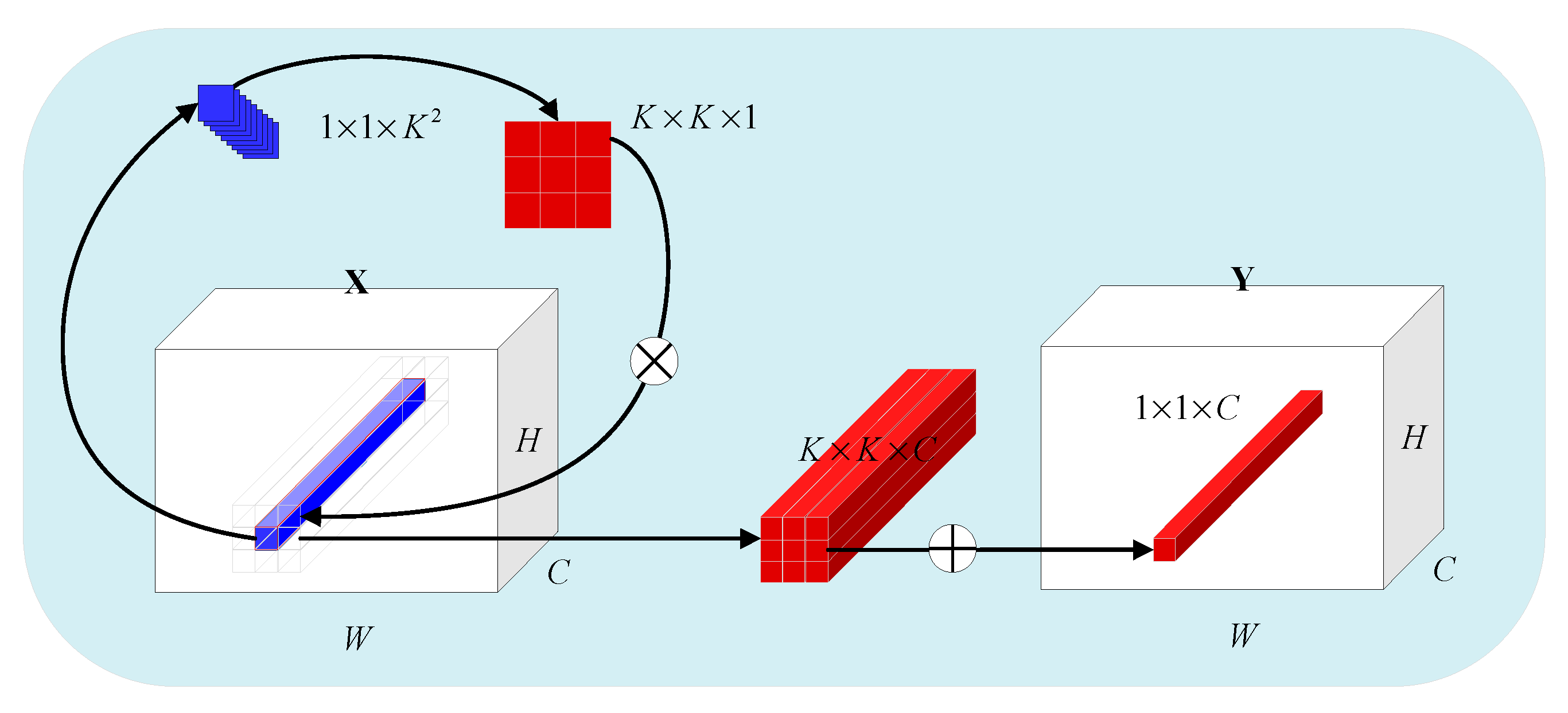
Figure 2.
Schematic diagram of GRU.
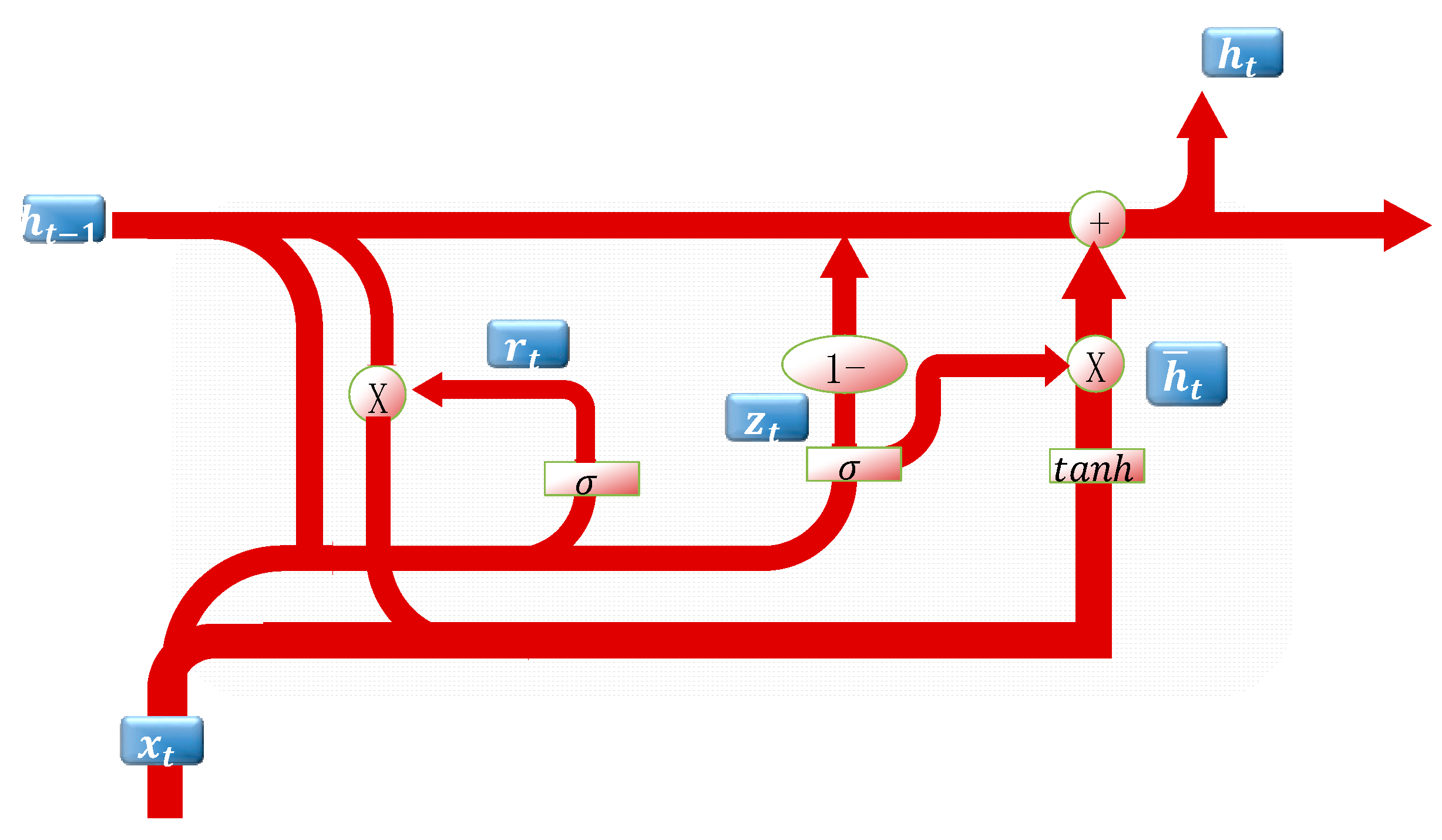
Figure 3.
Schematic diagram of InvGRU.
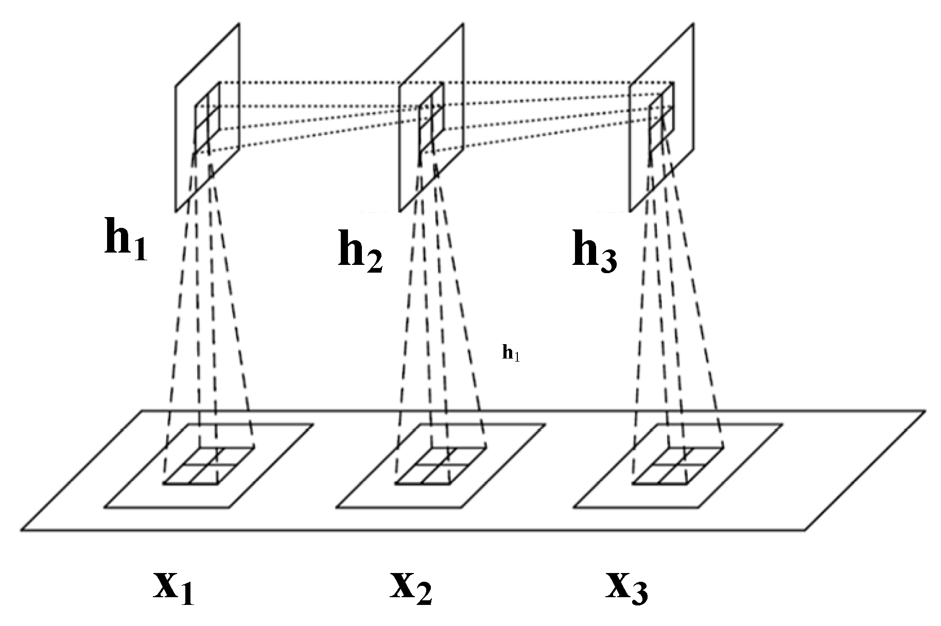
Figure 4.
InvGRU-based DL framework.
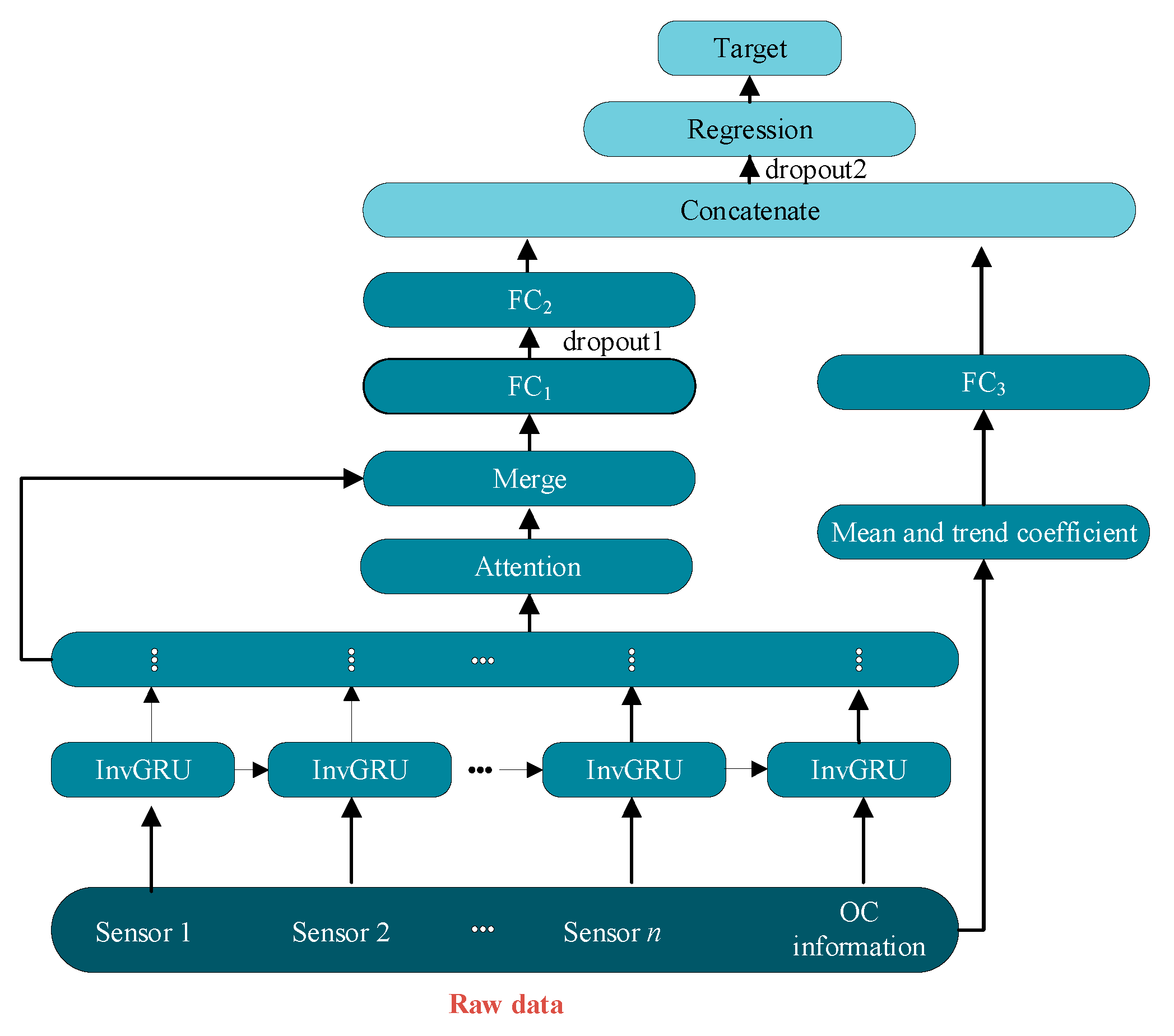
Figure 5.
The curves of the two evaluation indexes.
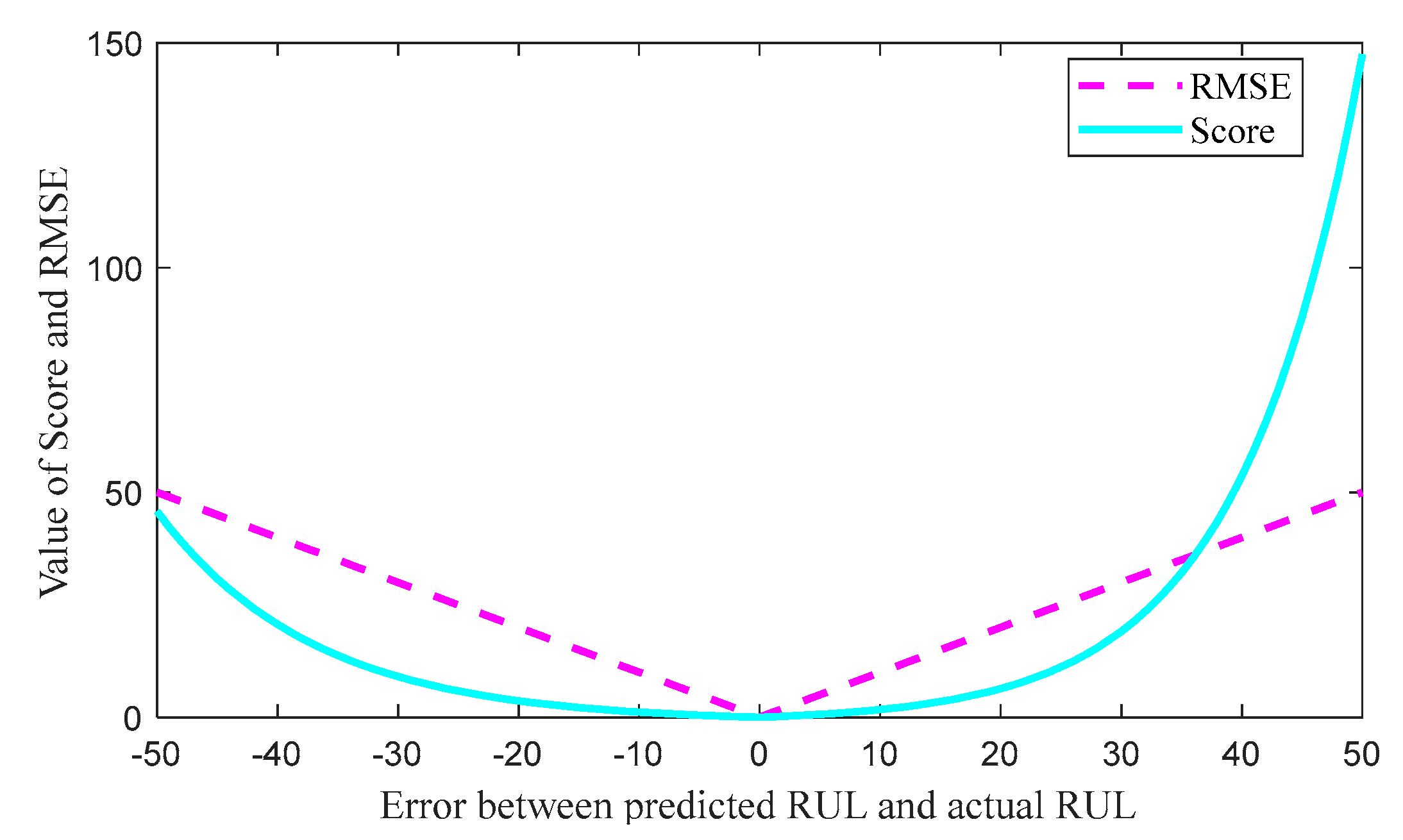
Figure 6.
Diagram of the aircraft engine.
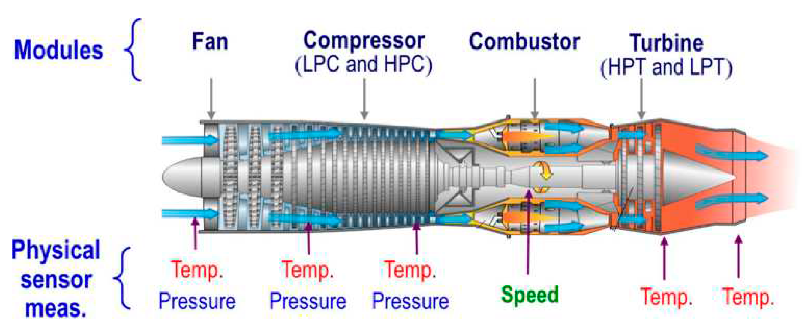
Figure 7.
Processing of data segmentation.
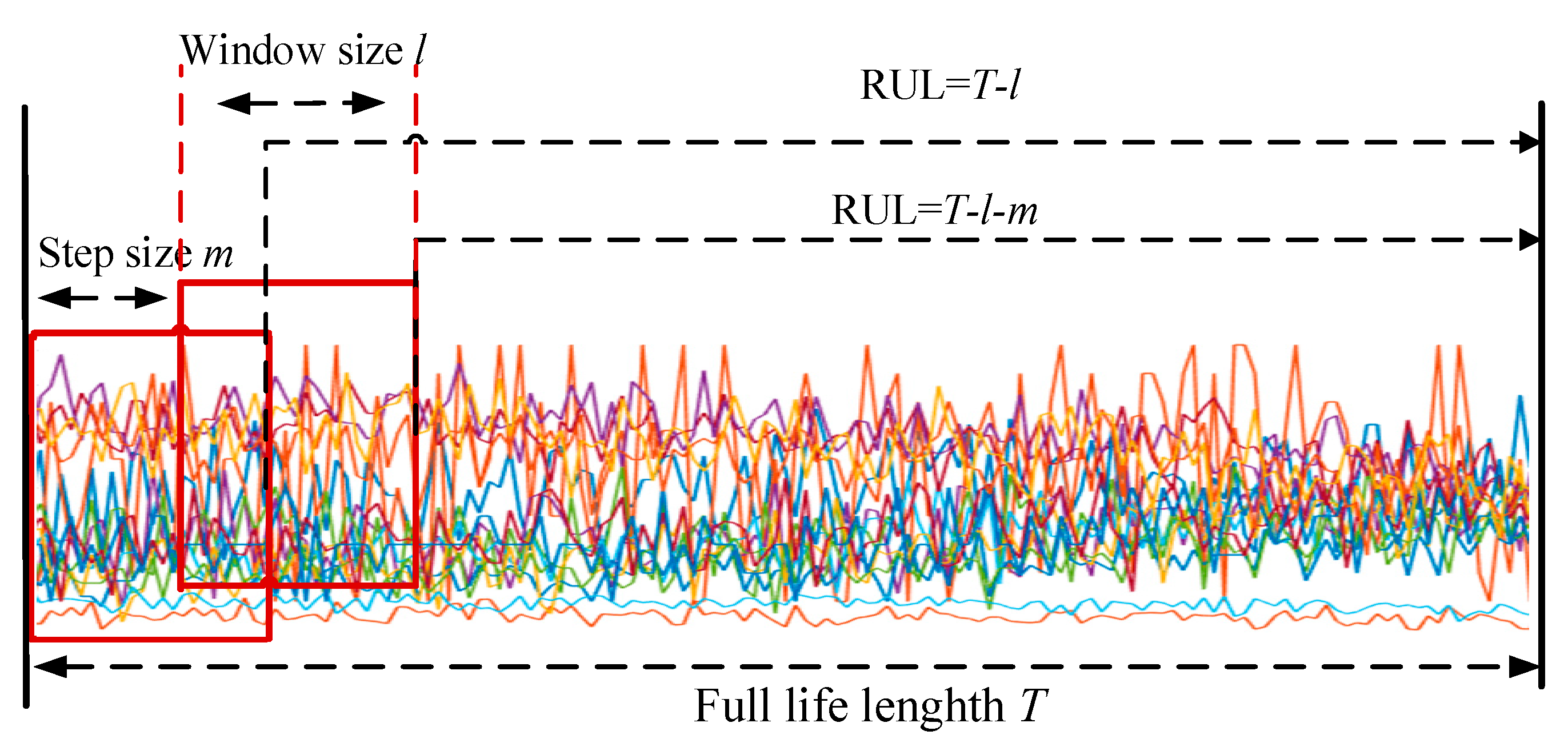
Figure 8.
RUL prediction performance on FD001.
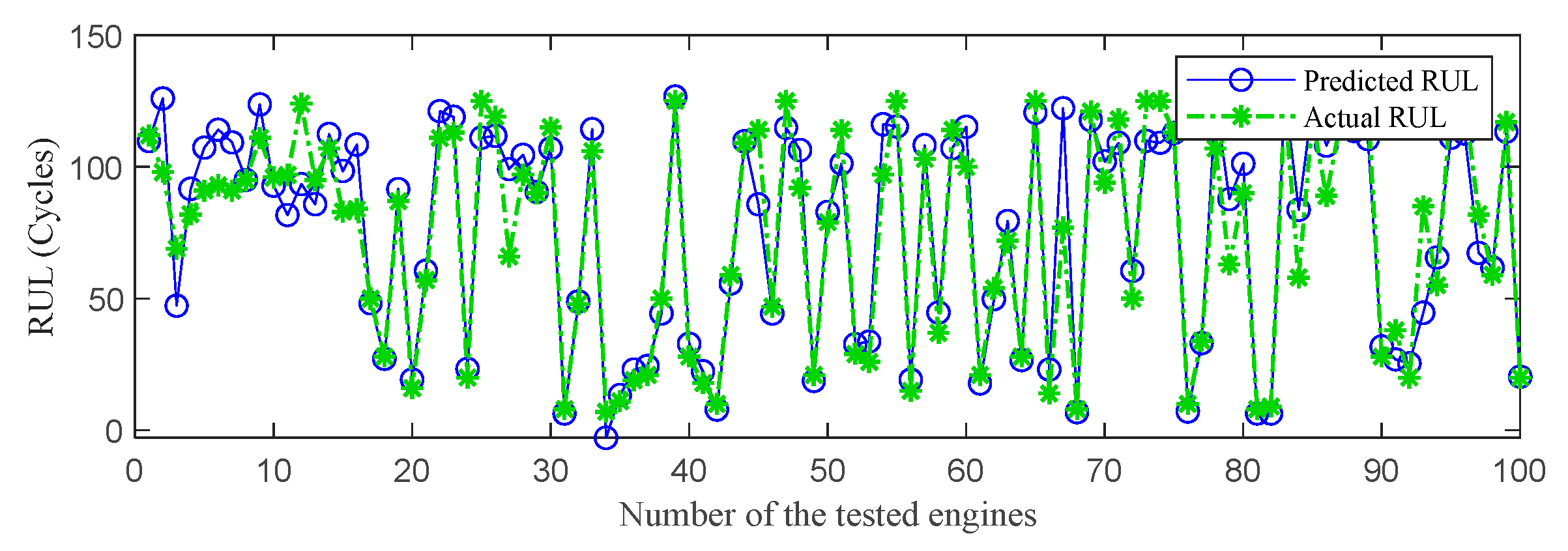
Figure 9.
RUL prediction performance on FD002.
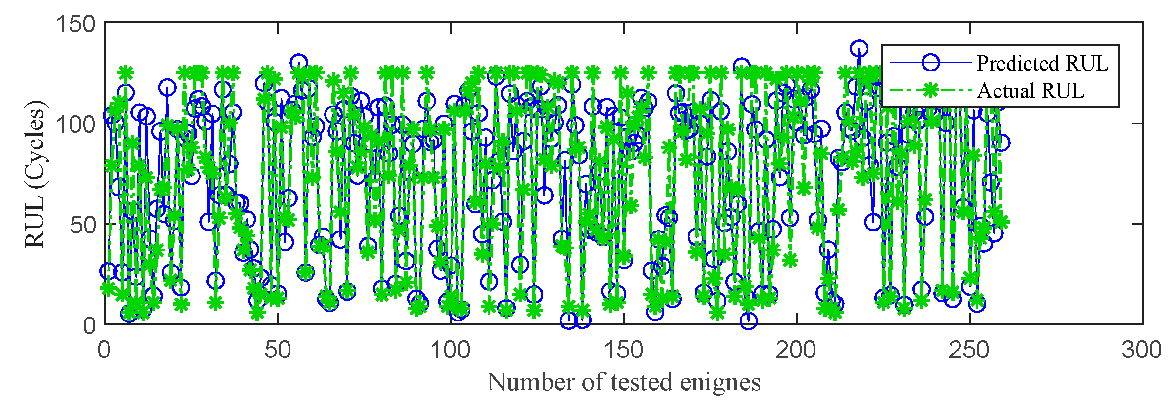
Figure 10.
RUL prediction performance on FD003.
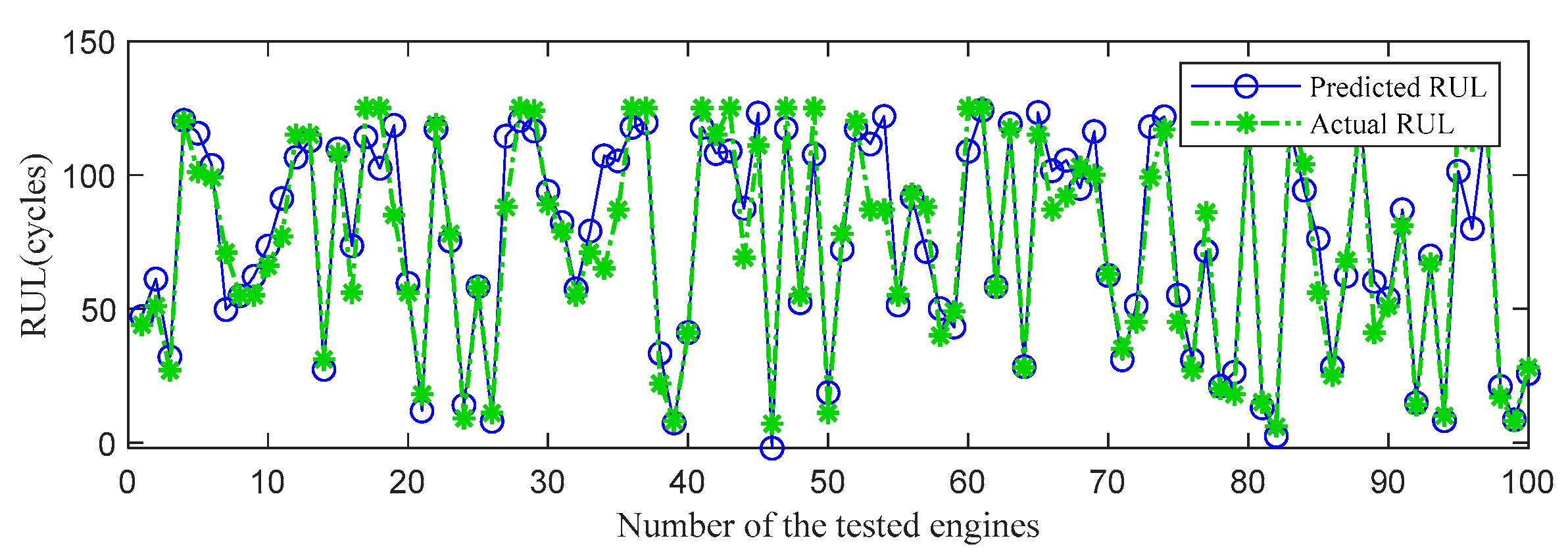
Figure 11.
RUL prediction performance on FD004.
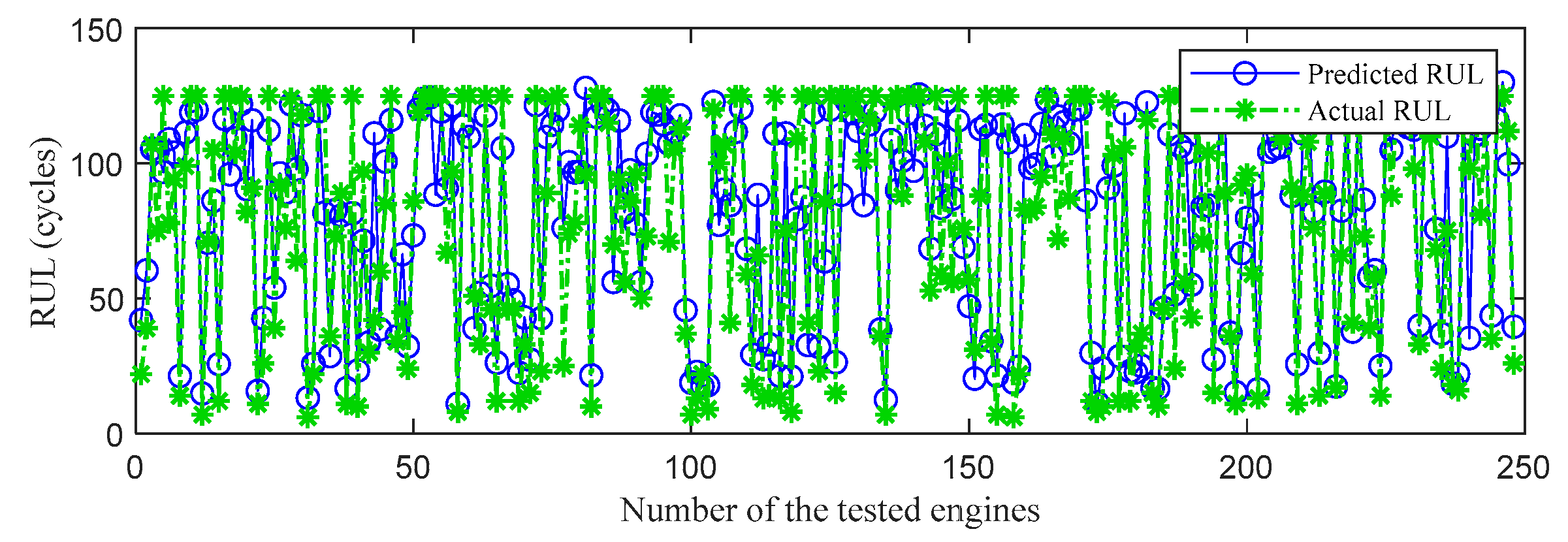
Figure 12.
RUL prediction performance of engines of FD001 ((a) engine # 46, (b) engine # 58, (c) engine # 66, and (d) engine # 92).
Figure 12.
RUL prediction performance of engines of FD001 ((a) engine # 46, (b) engine # 58, (c) engine # 66, and (d) engine # 92).
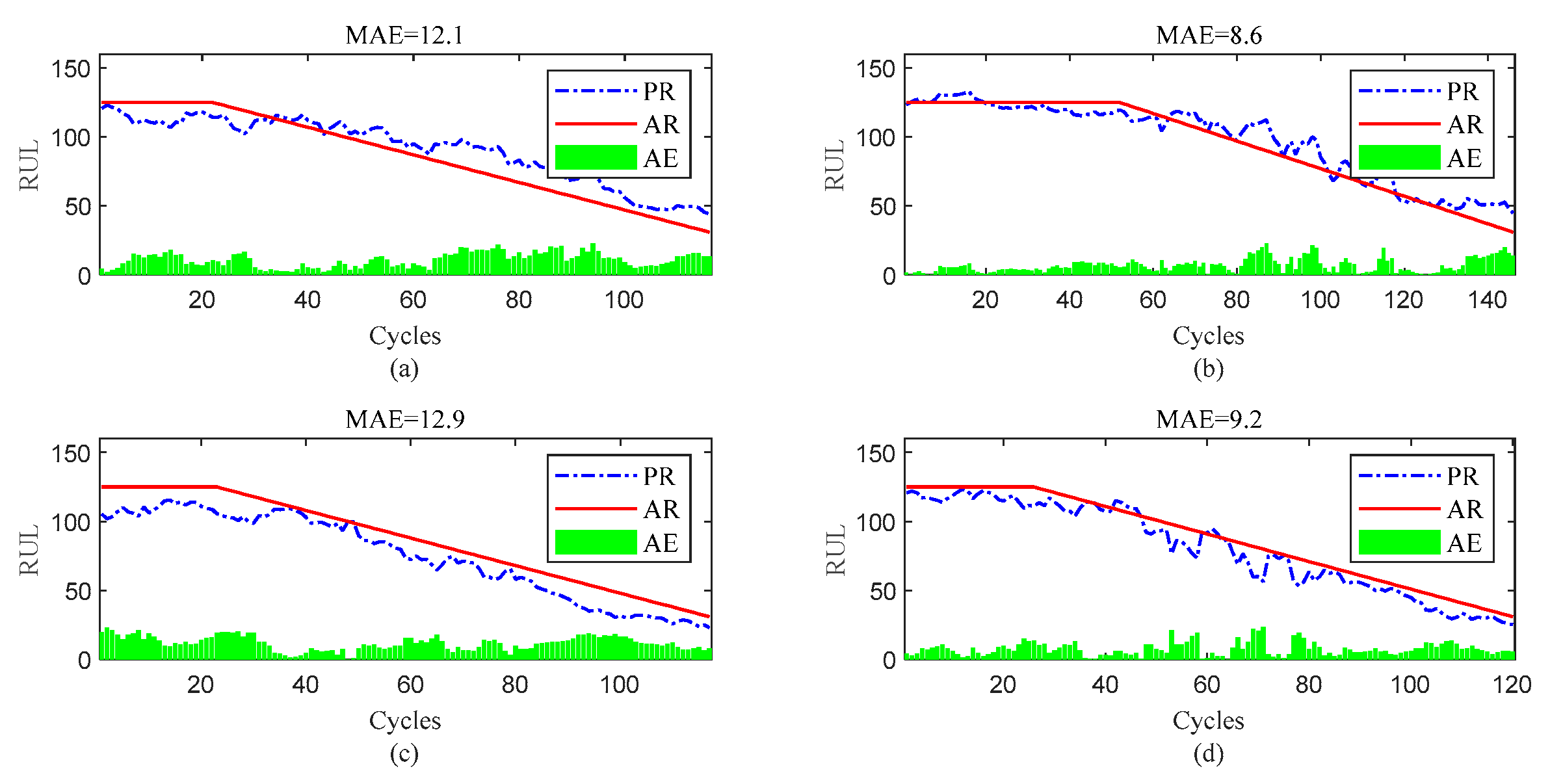
Figure 13.
RUL prediction performance of engines of FD002 ((a) engine # 9, (b) engine # 45, (c) engine # 150, and (d) engine # 182).
Figure 13.
RUL prediction performance of engines of FD002 ((a) engine # 9, (b) engine # 45, (c) engine # 150, and (d) engine # 182).
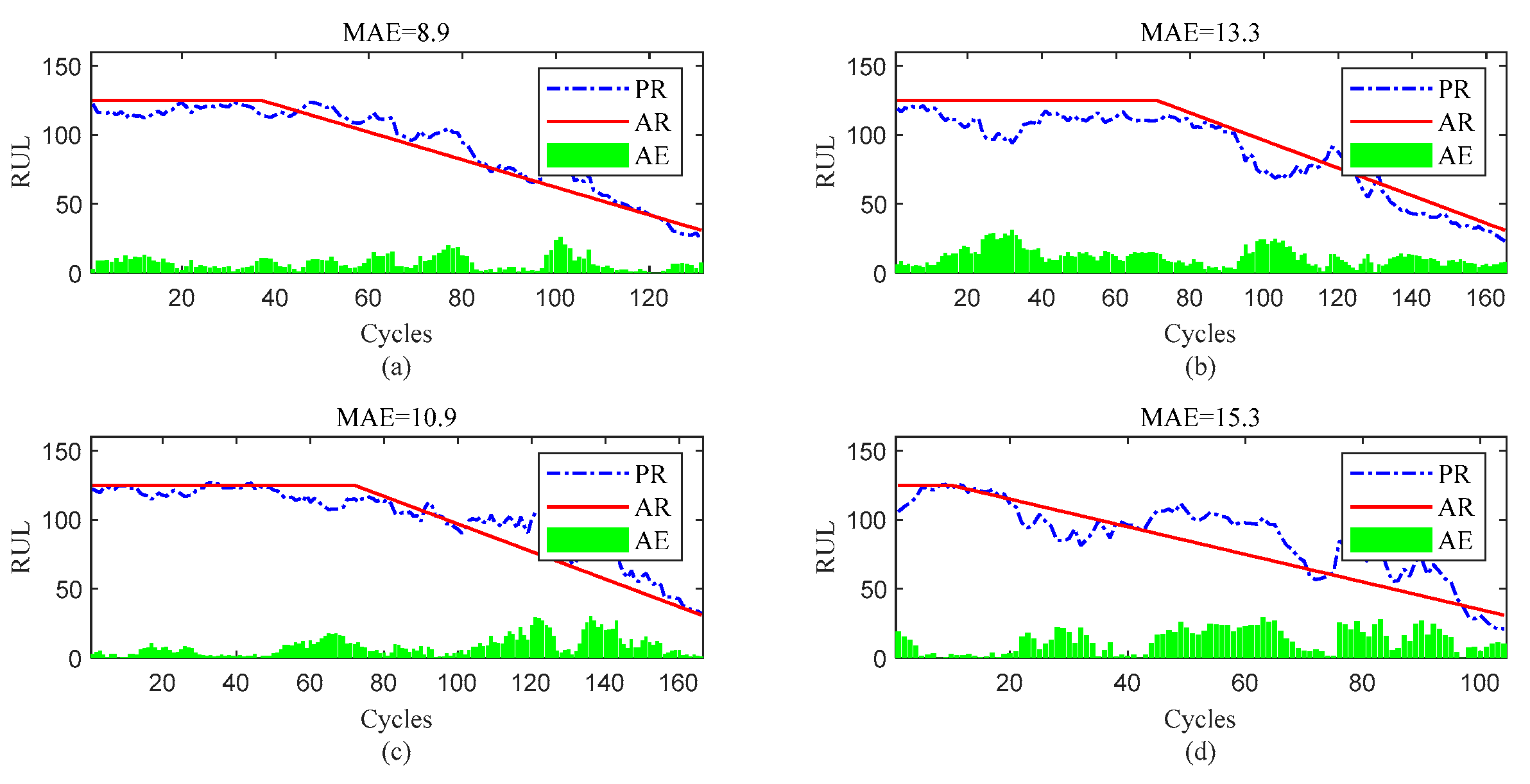
Figure 14.
RUL prediction performance of engines of FD003((a) engine # 25, (b) engine # 38, (c) engine # 75, and (d) engine # 92).
Figure 14.
RUL prediction performance of engines of FD003((a) engine # 25, (b) engine # 38, (c) engine # 75, and (d) engine # 92).
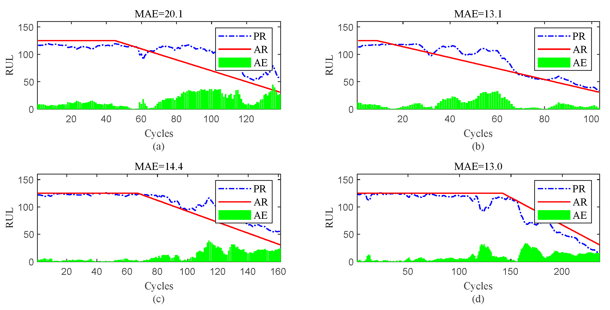
Figure 15.
RUL prediction performance of engines of FD004 ((a) engine # 35, (b) engine # 68, (c) engine # 100, and (d) engine # 151).
Figure 15.
RUL prediction performance of engines of FD004 ((a) engine # 35, (b) engine # 68, (c) engine # 100, and (d) engine # 151).
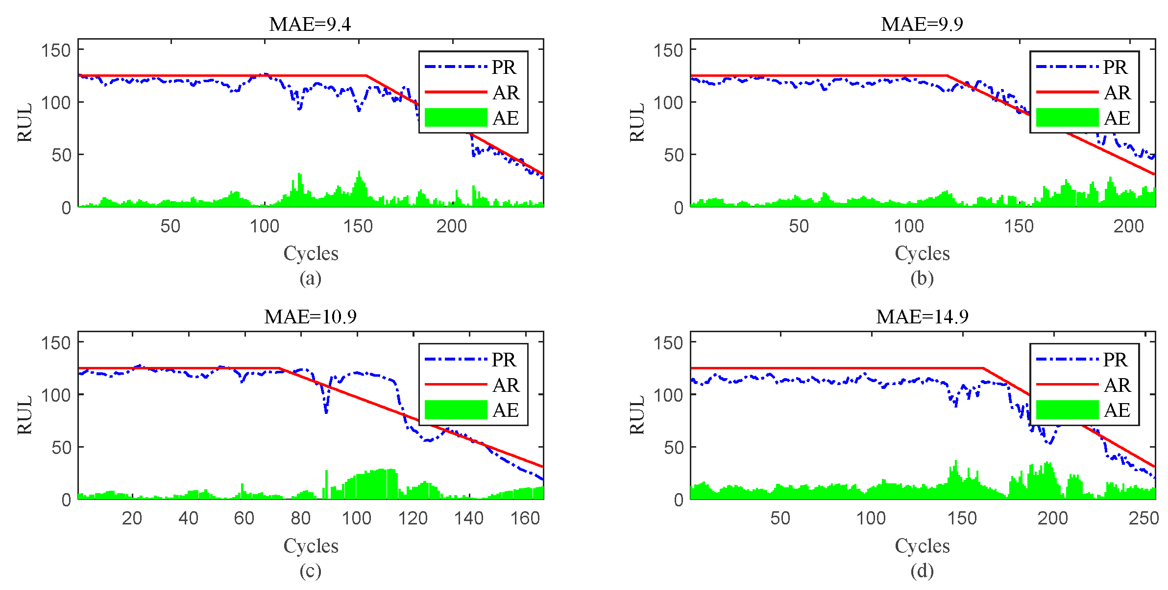

Table 1.
the hyper-parameters of the prosed DL framework based on InvGRU
| Sub layer | Hyperparameter value | Sub layer | Hyperparameter value |
|---|---|---|---|
| InvGRU | 70 | Regression (Linear) | 1 |
| FC1 (Relu) | 30 | Learning rate | 0.005 |
| FC2 (Relu) | 30 | Dropout1 | 0.5 |
| FC3 (Relu) | 10 | Dropout2 | 0.3 |
Table 2.
The details of dataset C-MAPSS
| Subset | FD001 | FD002 | FD003 | FD004 |
|---|---|---|---|---|
| Total number of engines | 100 | 260 | 100 | 249 |
| Operating condition | 1 | 6 | 1 | 6 |
| Type of fault | 1 | 1 | 2 | 2 |
| Maximum cycles | 362 | 378 | 525 | 543 |
| Minimum cycles | 128 | 128 | 145 | 128 |
Table 3.
Sensors of C-MAPSS
| number | symbol | description | unit | trend | number | symbol | description | unit | trend |
|---|---|---|---|---|---|---|---|---|---|
| 1 | T2 | Total fan inlet temperature | ºR | ~ | 12 | Phi | Fuel flow ratio to Ps30 | pps/psi | ↓ |
| 2 | T24 | Total exit temperature of LPC | ºR | ↑ | 13 | NRf | Corrected fan speed | rpm | ↑ |
| 3 | T30 | HPC Total outlet temperature | ºR | ↑ | 14 | NRc | Modified core velocity | rpm | ↓ |
| 4 | T50 | Total LPT outlet temperature | ºR | ↑ | 15 | BPR | bypass ratio | -- | ↑ |
| 5 | P2 | Fan inlet pressure | psia | ~ | 16 | farB | Burner gas ratio | -- | ~ |
| 6 | P15 | Total pressure of culvert pipe | psia | ~ | 17 | htBleed | Exhaust enthalpy | -- | ↑ |
| 7 | P30 | Total outlet pressure of HPC | psia | ↓ | 18 | NF_dmd | Required fan speed | rpm | ~ |
| 8 | Nf | Physical fan speed | rpm | ↑ | 19 | PCNR_dmd | Modify required fan speed | rpm | ~ |
| 9 | Nc | Physical core velocity | rpm | ↑ | 20 | W31 | HPT coolant flow rate | lbm/s | ↓ |
| 10 | Epr | Engine pressure ratio | -- | ~ | 21 | W32 | LPT coolant flow rate | lbm/s | ↓ |
| 11 | Ps30 | HPC outlet static pressure | psia | ↑ |
Table 4.
The RUL prediction comparisons of different methods on subset FD001and FD002.
| Model | FD001 | FD002 | ||
|---|---|---|---|---|
| Score | RMSE | Score | RMSE | |
| Cox’s regression [34] | 28616 | 45.10 | N/A | N/A |
| SVR [39] | 1382 | 20.96 | 58990 | 41.99 |
| RVR [39] | 1503 | 23.86 | 17423 | 31.29 |
| RF [39] | 480 | 17.91 | 70456 | 29.59 |
| CNN [40] | 1287 | 18.45 | 17423 | 30.29 |
| LSTM [42] | 338 | 16.14 | 4450 | 24.49 |
| DBN [41] | 418 | 15.21 | 9032 | 27.12 |
| MONBNE [41] | 334 | 15.04 | 5590 | 25.05 |
| LSTM+attention+handscraft feature [20] | 322 | 14.53 | N/A | N/A |
| Acyclic Graph Network [43] | 229 | 11.96 | 2730 | 20.34 |
| AEQRNN [34] | N/A | N/A | 3220 | 19.10 |
| MCLSTM-based[4] | 260 | 13.21 | 1354 | 19.82 |
| SMDN [14] | 240 | 13.72 | 1464 | 16.77 |
| Proposed | 238 | 12.34 | 1205 | 15.59 |
Table 5.
The RUL prediction comparisons of different methods on subset FD003 and FD004.
| Model | FD003 | FD004 | ||
|---|---|---|---|---|
| Score | RMSE | Score | RMSE | |
| Cox’s regression [34] | N/A | N/A | 1164590 | 54.29 |
| SVR [39] | 1598 | 21.04 | 371140 | 45.35 |
| RVR [39] | 17423 | 22.36 | 26509 | 34.34 |
| RF [39] | 711 | 20.27 | 46568 | 31.12 |
| CNN [40] | 1431 | 19.81 | 7886 | 29.16 |
| LSTM [42] | 852 | 16.18 | 5550 | 28.17 |
| DBN [41] | 442 | 14.71 | 7955 | 29.88 |
| MONBNE [41] | 422 | 12.51 | 6558 | 28.66 |
| LSTM+attention+handscraft feature [20] | N/A | N/A | 5649 | 27.08 |
| Acyclic Graph Network [43] | 535 | 12.46 | 3370 | 22.43 |
| AEQRNN [34] | N/A | N/A | 4597 | 20.60 |
| MCLSTM-based[4] | 327 | 13.45 | 2926 | 22.10 |
| SMDN [14] | 305 | 12.70 | 1591 | 18.24 |
| Proposed | 292 | 13.12 | 1020 | 13.25 |
Table 6.
The comparisons of different methods for RUL prediction b based on C-MAPSS dataset
| Model | Mean performance | |
|---|---|---|
| RMSE | Score | |
| Cox’s regression [34] | 49.70 | 596603 |
| SVR [39] | 32.335 | 108277 |
| RVR [39] | 27.96 | 11716 |
| RF [39] | 24.72 | 29553 |
| CNN [40] | 24.42 | 7006 |
| LSTM [42] | 21.25 | 2797 |
| DBN [41] | 21.73 | 4461 |
| MONBNE [41] | 20.32 | 3225 |
| LSTM+attention+handscraft feature [20] | 20.80 | 2985 |
| Acyclic Graph Network [43] | 16.80 | 1716 |
| AEQRNN [34] | 19.85 | 3908 |
| MCLSTM-based[4] | 17.40 | 1216 |
| SMDN [14] | 15.36 | 900 |
| Proposed | 13.58 | 689 |
Disclaimer/Publisher’s Note: The statements, opinions and data contained in all publications are solely those of the individual author(s) and contributor(s) and not of MDPI and/or the editor(s). MDPI and/or the editor(s) disclaim responsibility for any injury to people or property resulting from any ideas, methods, instructions or products referred to in the content. |
© 2023 by the authors. Licensee MDPI, Basel, Switzerland. This article is an open access article distributed under the terms and conditions of the Creative Commons Attribution (CC BY) license (http://creativecommons.org/licenses/by/4.0/).
Copyright: This open access article is published under a Creative Commons CC BY 4.0 license, which permit the free download, distribution, and reuse, provided that the author and preprint are cited in any reuse.


