Dirichlet Process Log Skew-normal Mixture with Missing at Random Covariate in Insurance Claim Analysis

Minkun Kim; David Lindberg; Martin Crane; Marija Bezbradica

doi:10.20944/preprints202306.0098.v1

Preprint

Article

Dirichlet Process Log Skew-normal Mixture with Missing at Random Covariate in Insurance Claim Analysis

This version is not peer-reviewed.

Minkun Kim^*,David Lindberg,

Martin Crane,Marija Bezbradica

Minkun Kim^*,David Lindberg,

Martin Crane,Marija Bezbradica

This version is not peer-reviewed.

Downloads

116

Views

Comments

Submitted:

31 May 2023

Posted:

01 June 2023

You are already at the latest version

A peer-reviewed article of this preprint also exists.

Abstract

In actuarial practice, the modeling of total losses tied to a certain policy is a non-trivial task. Traditional parametric models to predict total losses have limitations due to complex distributional features such as extreme skewness, zero inflation, multi-modality, etc., and the lack of explicit solutions for log-normal convolution. In the recent literature, the application of the Dirichlet process mixture for insurance loss has been proposed to eliminate the risk of model misspecification biases; however, the effect of covariates as well as missing covariates in the modeling framework is rarely studied. In this article, we propose novel connections among covariate-dependent Dirichlet process mixture, log-normal convolution, and missing covariate imputation. Assuming an individual loss is log-normally distributed, we develop a log skew-normal Dirichlet process to approximate the log-normal sum. As a generative approach, our framework models the joint of outcome and covariates, which allows to impute missing covariates under the assumption of missingness at random. The performance is assessed by applying our model to several insurance datasets, and the empirical results demonstrate the benefit of our model compared to the existing actuarial models such as the Tweedie-based generalized linear model, generalized additive model, or multivariate adaptive regression spline.

Keywords:

Bayesian nonparametric model

;

heterogeneity

;

missing at random

;

log-normal sum approximation

;

aggregate insurance claims

;

clustering

;

generative model

Subject:

Computer Science and Mathematics - Probability and Statistics

1. Introduction

In short-term insurance contracts, predicting accurate aggregate claims is essential for major actuarial decisions such as pricing or reserving. However, it is often not easy to model the aggregate loss due to its complex distributional features such as high skewness, zero inflation, hump shape, multi-modality, etc. With the advance of the modern Bayesian paradigm and computing power, the development of full distribution of aggregate claims has been studied and applied in actuarial practice. In particular, because of its considerable flexibility, a Bayesian nonparametric (BNP) approach has been gradually recognized to solve distributional conundrums in an insurance context. For instance, Hong and Martin (2018) [1] recently developed the Dirichlet process model as a BNP approach that maximizes the fitting flexibility of the full distribution for insurance loss, which obviates the chance of model misspecification bias. In this article, as an extension of their work, we aim to go beyond the search for the maximized fitting flexibility, focusing on the issues that arise from the presence of covariates and the aggregate outcome (total losses). The implication is that the predictive distribution for the expected aggregate claims developed under Hong and Martin’s Dirichlet process framework can be biased with the incorporation of covariate effects and log-normal convolution. For example, as covariates add new information that differentiates the data points of the outcome variable, a new structure can be introduced into the data space, and this increases the within-cluster heterogeneity [2]. Besides, the incorporation of missing covariates may exacerbate the existing heterogeneity. Additionally, assuming that the outcome variable describes the aggregate losses, rather than individual claim amounts, it is difficult to compute the log-normal convolution as it does not have a closed-form solution. In this regard, our study extends their work by addressing the following research questions:

RQ1. If an additional unobservable heterogeneity is introduced by the inclusion of covariates, what is the best method to capture the within-cluster heterogeneity in modeling the total losses, comparing several conventional approaches?
RQ2. If an additional estimation bias results from the use of the incomplete covariates under Missing At Random (MAR), what is the best way to increase the imputation efficiency, comparing several conventional approaches?
RQ3. If an individual loss is distributed with log-normal densities, what is the best way to approximate the sum of log-normal outcome variables, comparing several conventional approaches?

2. Discussion on Research Questions and Related Work

Let

Y_{i}, i = 1, 2, \dots, N

be the independent claim amount (reported by each policyholder for a single policy) random variable, defined on a common probability space (

Ω, F, P

) from a certain loss distribution such as log-normal. Let

X

be a vector of covariates, and

N (t)

be the total claim count denoting the number of individual claims for a single policy up to time t (policy period). The aggregate claim

S_{h} (t)

for a single policy, h, given time t can be expressed as a convolution:

S_{h} (t) = \sum_{i = 1}^{N (t)} Y_{i} = Y_{1} + Y_{2} + \dots + Y_{N (t)}

. At the end of the policy period t, let

\tilde{S} (t)

be the total aggregate claim amounts from the total policies received by an insurer, then:

\tilde{S} (t) = \sum_{h = 1}^{H} S_{h} (t) = S_{1} (t) + S_{2} (t) + \dots + S_{H} (t)

in which H is the total number of policies on the contracts. Note that both convolutions described so far are built upon the assumption that the summands -

Y_{i}, i = 1, 2, \dots, N (t)

and

S_{h}, h = 1, 2, \dots, H

- are mutually independent and identically distributed with log-normal densities (to maintain homogeneity of each loss).

However, the involvement of covariates and the lack of closed-form solutions for the log-normal sum bring about several challenges that violate the assumptions for an accurate estimation of the total aggregate loss

\tilde{S} (t)

. To begin with, the use of covariates gives rise to an additional within-cluster heterogeneity. Kass et al.(2008) [3] describes a standard aggregate loss modeling principle denoting that the expected aggregate claims

E [S_{h}]

is obtained by the product of the mean claim counts and severities:

E [S_{h}] = E [N] E [Y]

. With the inclusion of covariates

X

, a new unknown structure or heterogeneity is introduced into the data space of

Y_{i}

, which means that

Y_{1} | X_{1}, Y_{2} | X_{2}, \dots, Y_{N} | X_{N}

within a single policy can still be independent, but cannot be identically distributed. Therefore,

E [S_{h} | X] \neq E [N | X] E [Y | X]

, and the total aggregate loss

\tilde{S} (t)

becomes difficult to compute with the conventional collective risk modeling approach. In addition, assuming that the severity

Y_{i}

follows a log-normal distribution, the computation of

\tilde{S} (t)

becomes quite difficult as its convolution

S_{h}

is not known to have a closed-form [4]. Another challenge is the missing covariates in

S_{h} | X

. As shown by Ungolo et al.(2020) [5], the missing covariates under the missingness at random (MAR) assumption lead to the biased parameter estimations because the uncertainty in the estimation results of the parameters describing the outcome Y is heavily affected by the quality of covariates

X

. Again, in this case,

\tilde{S} (t)

cannot be computed properly.

Compounding all this, we propose the Dirichlet process log skew-normal mixture to model the

S_{h} | X

. We consider the Dirichlet process framework to cope with the within-cluster heterogeneity as suggested by Hong and Martin (2018); Braun et al.(2016) [1,6] while employing the log skew-normal approximation studied by Li (2008) [7] to compute each

S_{h} | X

, the sum of log-normal random variables

\sum_{i = 1}^{N (t)} Y_{i} | X

. When it comes to the problem of missing covariates, we exploit the generative capability of the Dirichlet process to capture the latent structure of data, which allows for a rigorous statistical treatment of MAR covariates.

2.1. Can Dirichlet Process Capture the Heterogeneity and Bias?: RQ1, RQ2

In Figure 1,

Y_{i}

refers to individual claim amount and each

S_{h}

represents a total claim amount defined by a unique policy (cluster h) as a homogeneous distribution. Although an insurer can collect the aggregate loss data

S_{h}

for each policy cluster given policy period t, individual policyholders (in different risk classes) can raise more than one claim (i.e. random

N_{h} (t)

) at any time over a fixed time horizon t, and their corresponding claim amounts (i.e. random

Y_{h}^{*}

) will not be known in advance. Hence, the unsettled liability information of

Y_{h}^{*}

from certain policyholders always renders

S_{h}

incomplete, which is often translated into the challenge of their inherent stochasticity. In addition, the new claims

Y_{h}^{*}

raised from unknown risk classes can trigger inherent heterogeneity across unique clusters as well. To make matters worse, if introducing covariates

X

to better understand the different risk classes, one might introduce an additional source of heterogeneity into the scene, which prevents each cluster from being identically distributed.

With respect to this, Hong and Martin (2018) [1] propose the concept of the loss distribution mixture for each cluster based on the Dirichlet process framework. The main idea behind the Dirichlet process mixture (DPM) is to produce a single master distribution to model stochasticity in

S_{h}

with the help of an infinite dimensional parametric structure and the probabilistic simulations of clustering scenarios. Braun et al.(2006) [6] articulates how the DPM automatically captures unobservable heterogeneity such as intracorrelation between claim amounts

Y_{i}

in the different risk classes without specifying the number of the classes upfront. In short, no matter how complex the distribution of the data is, the DPM is capable of accommodating any distributional properties - multi-modes, skewness, heavy tails, etc. - resulting from unobservable heterogeneity; and therefore, dramatically minimizes model misspecification biases.

With the inclusion of the covariates, the DPM offers a useful bedrock for a MAR treatment. As a generative modeling approach, the DPM models both outcomes

S_{h}

and covariates

X

jointly to produce cluster memberships. This is used as key knowledge to identify the latent structure of the data. For example, in the domain of medicine research, Roy et al. (2018) [8] develop a novel imputation strategy for the MAR covariate, using the latent structure unraveled by the DPM and the other covariate knowledge available. A further survey of imputation methods based on the Nonparametric Bayesian framework can be found in Si and Reiter (2013) [9] and references therein.

2.2. Can Log Skew-Normal Mixture Approximate the Log-Normal Convolution?: RQ3

The log-normal distribution has been considered a suitable claim amount

Y_{i}

distribution due to its non-negative support, right-skewed curve, and moderately heavy tail to accommodate some outliers. However, if generalizing the individual claim amount

Y_{i}

by introducing a log-normal distribution, the convolution computation for

S_{h}

fails because the exact closed form for the log-normal sum is unknown.

Furman et al. (2020) [10] present several existing methods for the log-normal sum approximation that have been studied in the literature. This includes the moment matching approximation approaches such as Minimax approximation, Least squares approximation, Log shifted gamma approximation, and Log skew-normal approximation. The distance minimization approaches - Minimax approximation or Least squares approximation - described by Beaulieu and Xie (2003); Zhao and Ding (2007) [4,11] are conceptually simple, but they require to fit the entire cumulative densities to the sum of claim amounts, which can be computationally expensive and easy to fail when the number of the summands

Y_{i}

increases. The Log shifted gamma approximation suggested by Lam and Le-Ngoc (2007) [12] has less strict distributional assumptions, but it is not very accurate at the lower region of the distribution. In our study, special attention is paid to the possibility of the Log skew-normal approximation method for the sake of simplicity. A skew-normal distribution as an extension of a normal distribution has a third parameter to naturally explain skewness apart from the other parameters (for a location and spread). Li (2008) [7] points out that one can exploit the third parameter of the skew-normal distribution to capture different skewness levels of each summand. Taking the log of skew-normal densities, we can approximate

S_{h}

, the sum of the log-normal

Y_{i}

. Using the log skew-normal as the underlying distribution for

S_{h}

in the DPM framework, one can eliminate the need to compute the cumulative density curve, and its closed-form density and the optimal distribution parameters for

S_{h}

can be easily obtained by the moment matching technique. For further details, see Li (2008) [7] and the references contained within.

2.3. Our Contribution and Paper Outline

The contribution of this study is as follows: first, using the Bayesian nonparametric framework, we propose solutions to the two major challenges of the aggregate claim

S_{h}

computation - 1) heterogeneity in the log-normal random variable

Y_{i}

, 2) lack of closed-form of the sum of log-normal random variables

Y_{i}

- in a more unified fashion. Second, we introduce covariates

X

into the aggregate claim modeling framework, taking into account the adverse impact triggered by the covariates

X

. This includes the added heterogeneity across

Y_{i}

and the missing information fed by MAR covariates

X

. To our knowledge, there have been no previous attempts to either estimate the log skew-normal mixture within the DPM framework or use the DPM to handle the MAR covariate in the insurance loss modeling.

The rest of the paper is structured as follows. In Section 3, we describe the proposed modeling framework for

S_{h}

, assuming log-normal distributed

Y_{i}

and the inclusion of both continuous and discrete covariates

X

. This section also presents our novel imputation approach for the MAR covariate within the DPM framework. Section 4 clarifies the final forms of the posterior and predictive densities accordingly. Section 5 presents our empirical results, and validates our approach by fitting to two different datasets with different sample sizes drawn from the R package CASdatasets and the Wisconsin Local Government Property Insurance Fund (LGPIF). This is followed by a discussion in Section 6.

3. Model: DP Log Skew-Normal Mixture for $S_{h} | X$

3.1. Background

Consider that there are multiple unknown risk classes (clusters) across the claim

Y_{i}

information within each policy, and then the individual aggregate claims

S_{h}

for the policy h would have diverse characteristics that cannot be explained by fitting a single log skew-normal distribution. In order to approximate the distribution that captures such diverse characteristics in

S_{h}

, we seek to investigate diverse clustering scenarios. To this end, as suggested by Hong and Martin (2018) [1], we exploit the infinite mixture of log skew-normal clusters and their complex dependencies by employing a Dirichlet process. The Dirichlet process produces a distribution over clustering scenarios (with clustering parameters).

\begin{matrix} {θ_{j}, ω_{j}} & \sim G \\ G & \sim D P (α, G_{0}) \end{matrix}

where G denotes the clustering scenarios, and the important components of G are

$θ_{j}$ : the parameters of the outcome variable defined with cluster j.
$ω_{j}$ : the parameter of the cluster weights defined with cluster j.

G, as a single realization of the joint cluster probability vector

{G (A_{1}), G (A_{2}) \dots}

sampled from the DPM model, takes independent partitions

A_{1}, A_{2}, \dots

of the sample space

⋃_{k = 1}^{\infty} A_{k} = A

of the support of

G_{0}

. By sufficient simulations of G, the Dirichlet process investigates all possible clustering scenarios rather than relying on a single best guess. The overall production of G is controlled with two parameters - a precision

α

and a base measure

G_{0}

. The precision

α

controls a variance of sampling G in the sense that larger

α

generates new clusters more often to account for the unknown risk classes. The base measure

G_{0}

, as the mean of DP(

α, G_{0}

), is a DP prior over the joint space of all parameters for the outcome model, covariate model, and the precision

α

, as shown in Ghosal (2010) [13].

Note that the original research on DPM by Hong and Martin (2018) [1] mainly focuses on the random cluster weights

ω_{j}

independent of the covariates

X

. On the other hand, in our model, the covariate effects are incorporated into the development of cluster weights

ω_{j}

. All calculations for the development of the DPM modeling components in this paper are based on the principles introduced by Ferguson (1973), Antoniak (1974), and Sethuraman (1994) [14,15,16].

3.2. Model Formulation with Discrete and Continuous Clusters

Let the outcome be

S = {S_{1}, S_{2}, \dots, S_{H}}

denoting the H different aggregate claims (incurred by the H different policies). We assume that the covariate

x_{1}

is binary, and the

x_{2}

is Gaussian, and then our baseline DPM model can be expressed as:

\begin{matrix} S_{h} | x_{1}, & x_{2}, β_{j}, σ_{j}^{2}, ξ_{j}, {\tilde{β}}_{j} \\ \sim δ (X^{T} {\tilde{β}}_{j}) 1 (S_{h} = 0) + [1 - δ (X^{T} {\tilde{β}}_{j})] L o g S N (X^{T} β_{j}, σ_{j}^{2}, ξ_{j}) \\ x_{1} | π_{j} & \sim B e r n (π_{j}) \\ x_{2} | μ_{j}, τ_{j}^{2} & \sim N (μ_{j}, τ_{j}^{2}) \\ {θ_{j}, w_{j}} & \sim G \\ G & \sim D P (α, G_{0}) \end{matrix}

(1)

where j is the risk class index;

θ_{j} = {β_{j}, σ_{j}^{2}, ξ_{j}, {\tilde{β}}_{j}

} describe the outcome model while

w_{j} = {π_{j}, μ_{j}, τ_{j}^{2}}

explains the covariate model.

S_{h}

is modeled as a mixture of a point mass at 0 and positive values distributed with log skew-normal density to address the complications of zero inflation in the loss data.

δ (X^{T} {\tilde{β}}_{j})

models the probability of the outcome being zero using a multivariate logistic regression. Variable Definitions section has a brief description of all parameters used in this study.

Considering a Dirichlet process log skew-normal mixture to house the multiple unknown risk classes in

S_{h}

, it is necessary to differentiate the forms of mixture components depending on the types of clusters it uses - the discrete and continuous. While keeping the inference of the cluster parameters to be data dominated, the DPM first develops discrete clusters based on the given claim information and then extrapolates certain unobservable clusters of claims by examining the heterogeneity (or hidden risk classes) of each cluster. In this process, the DPM develops new continuous clusters additionally and assesses them with some probabilistic decision-making algorithms, rendering the parameter estimations computationally efficient and asymptotically consistent [17].

The discrete mixture components (clusters) in the DPM framework have the standard form that is useful in accounting for the observed classes such as policy information for aggregate loss

S_{h}

[18]. In calculating the discrete cluster probabilities, we assume that the non-zero outcome and covariates are distributed with the densities denoted by

\begin{matrix} f_{L S N} (S_{h} | X_{h}^{T} β_{j}, σ_{j}^{2}, ξ_{j}) & = \frac{2}{S_{h} σ_{j}} ϕ (\frac{log S_{h} - X_{h}^{T} β_{j}}{σ_{j}}) \cdot Φ (ξ_{j} \cdot \frac{log S_{h} - X_{h}^{T} β_{j}}{σ_{j}}) \end{matrix}

(2a)

\begin{matrix} f_{B e r n} (x_{1} | π_{j}) & = π_{j}^{x_{1}} {(1 - π_{j})}^{1 - x_{1}} \end{matrix}

(2b)

\begin{matrix} f_{N} (x_{2} | μ_{j}, τ_{j}^{2}) & = \frac{1}{\sqrt{2 π τ_{j}^{2}}} exp \{- \frac{1}{2 τ_{j}^{2}} {(x_{2} - μ_{j})}^{2}\} \end{matrix}

(2c)

where

ϕ (\cdot)

and

Φ (\cdot)

are standard normal probability and cumulative density functions for the log skew-normal density. To model the outcome data

S_{h} | X_{h}

for the policy h, the DPM takes the general form of the mixture

f (S_{h} | X_{h}, θ) = \sum_{j = 1}^{J} ω_{j} (δ (X_{h}^{T} {\tilde{β}}_{j}) 1 (S_{h} = 0) + [1 - δ (X_{h}^{T} {\tilde{β}}_{j})] f_{L S N} (S_{h} | X_{h}, θ_{j}))

(3)

where J is the total number of mixture components (risk classes),

θ_{j} = {β_{j}, σ_{j}^{2}, ξ_{j}, {\tilde{β}}_{j}}

and

w_{j} = {π_{j}, μ_{j}, τ_{j}^{2}}

are the outcome and covariate parameters to explain the risk clusters, and

ω_{j}

, functions of covariates:

ω_{j} (X_{h} | w_{j})

, are the cluster components weights (mixing coefficient) satisfying

\sum_{j = 1}^{J} ω_{j} = 1

However, when the DPM is extended as

j \to \infty

, the new continuous clusters are introduced by the

G_{0}

(with its infinite-dimensional parametric structure) in order to address the additional unknown risk classes. This assesses the within-class heterogeneity in

S_{h}

by confronting the current discrete clustering result and investigating the homogeneity more closely. As the new clusters are considered countably infinite, their corresponding forms of the outcome and covariate models to obtain the continuous cluster are given by

\begin{matrix} f_{0} (S_{h} | X_{h}) & = \int f (S_{h} | X_{h}, θ) d G_{0} (θ) \end{matrix}

(4a)

\begin{matrix} f_{0} (x_{1}) & = \int f_{B e r n} (x_{1} | w) d G_{0} (w) \end{matrix}

(4b)

\begin{matrix} f_{0} (x_{2}) & = \int f_{N} (x_{2} | w) d G_{0} (w) \end{matrix}

(4c)

They are also known as a “parameter-free outcome model" and a “parameter-free covariate model" respectively to develop the new continuous cluster mixture. Given a collection of outcome-covariate data pairs

D = {S_{h}, X_{h}}_{h = 1}^{H}

, the DPM puts together the current discrete clusters and new continuous clusters to update the mixture form in Equation (3), with help of Monte Carlo Markov Chain (using sufficiently simulated samples of the major parameters

θ_{j}, w_{j}

). Consequently, the sample G described in Equation (1) becomes

G = f (S_{h} | X_{h}, D) = \sum_{j = 1}^{\infty} ω_{j} \cdot δ_{z_{j}}

where

δ_{z_{j}}

denotes both discrete and continuous cluster densities as point mass distributions at the random locations sampled from

G_{0}

. Aligned with such flexible cluster development, the form of the predictive distribution can be molded based on the knowledge extracted from G, as follow:

f (S_{h} | X_{h}, θ, w, α) = \frac{ω_{J + 1}^{*}}{ω_{J + 1}^{*} + \sum_{j = 1}^{J} ω_{j}^{*}} \cdot f_{0} (S_{h} | X_{h}) + \frac{\sum_{j = 1}^{J} ω_{j}^{*} \cdot f (S_{h} | X_{h}, θ_{j})}{ω_{J + 1}^{*} + \sum_{j = 1}^{J} ω_{j}^{*}}

(5)

and the finalized cluster weights in Equation (5) are secured through computing these two sub-models below for discrete and continuous cluster weights respectively which reflect the properties of the clusters and relevant covariates.

\begin{matrix} ω_{J + 1}^{*} & = \frac{α}{α + H} \cdot f_{0} (x_{1}, x_{2}) \end{matrix}

(6a)

\begin{matrix} ω_{j}^{*} & = \frac{n_{j}}{α + H} \cdot f (x_{1}, x_{2} | w_{j} = (π_{j}, μ_{j}, τ_{j}^{2})) \end{matrix}

(6b)

where

α

is the precision parameter to control the acceptance chances of the new clusters,

n_{j}

is the number of observations in cluster j,

f_{0} (X)

is the parameter-free covariate model in Equation (4b, 4c) to support the new continuous clusters, and

f (X | w_{j})

is the covariate model to support the current discrete clusters. Note that instead of the popular stick-breaking scheme used by Hong and Martin (2018) [1], the cluster weights are obtained based on the covariate models of

x_{1}, x_{2}

that explain the outcome

S_{h}

The simulated outcome model

f (S_{h} | X_{h}, D) = \sum_{j = 1}^{\infty} ω_{j} \cdot δ_{z_{j}}

and its predictive model in Equation (5) show that although the DPM framework allows infinite-dimensional modeling, the dimension of the sampling output G is adaptive as it is a mixture with at most finite components determined by data itself (e.g. its dimension cannot be greater than the total sample size H). This gives the model flexibility, and throughout such modeling flexibility, the G can become the comprehensive mixture distribution for

S_{h}

, accommodating all distributional properties of the given claims as well as the additional unknown claims.

3.3. Modelling $S_{h} | X_{h}$ with Complete Case Covariate

The joint posterior update for the outcome and covariate parameters -

θ_{j}, w_{j}

- in Equation (5,6) can be made through a Gibbs Sampler. Using the conditional distribution of the unobservable variables given the observed data, the Gibbs sampler can obtain draws from the analytically intractable posterior distribution of the parameters [20]. Let the cluster-index

j = 1, 2, \dots, J

for the observation h be

s_{h}

. The parameter inference steps to ensure convergence are described below.

Step.1

Initialize the cluster membership and the main parameters:

(a): First the cluster membership $j = 1, \dots, J$ is initialized by some clustering methods such as hierarchical clustering or k-means, etc. This step provides an initial clustering of the data ( $S_{h}, X_{h})$ as well as the initial number of clusters.
(b): Next, after all observations have been assigned to a particular cluster $j = 1, 2, \dots, J$ , we can then update the parameters $α$ and ( $θ_{j}, w_{j}$ ) for each cluster. This is done using the posterior densities denoted by $p (α | J), p (θ | S_{h}, X_{h})$ , and $p (w | X_{h})$ in which ( $S_{h}, X_{h}$ ) represent all observations in cluster j.

Step.2

Loop through the Gibbs sampler and new continuous cluster selection:

Once the cluster memberships and parameters are initialized, we then loop through the Gibbs sampler many times (e.g.

M = 100, 000

iterations) where the algorithm alternates between updating the cluster membership for each observation and updating the parameters given the cluster partitioning. Each iteration might give a slightly different selection of the new clusters based on the Polya Urn scheme [20], but the log-likelihood calculated at the end of each iteration can help keep track of the convergence of the selections. A detailed description of each iteration is given in Algorithm (A2) in Appendix B. The term

p (s_{h} | s_{- h})

on lines 6 and 9 in Algorithm (A2) is the Chinese Restaurant process [19] posterior value given by

p (s_{h} | s_{- h}) = \{\begin{matrix} c \cdot \frac{n_{j}^{- h}}{α + H - 1}, & for record h entering into existing cluster : s_{h} = j . \\ c \cdot \frac{α}{α + H - 1}, & for record i entering into a new cluster : s_{h} = J + 1 . \end{matrix}

(7)

where c is a scaling constant to ensure that the probabilities sum to 1, and

s_{- h}

is the collection of cluster indices

(s_{1}, s_{2}, \dots, s_{h - 1}, s_{h + 1}, \dots, s_{H})

assigned to every observation without the cluster index

s_{h}

of the observation h. As shown in Equation (7), the larger

α

results in a higher chance of developing the new continuous cluster and adding to the collection of the existing discrete clusters. The forms of the prior and posterior densities used to simulate the main parameters

(θ_{j}^{*}, α^{*}, w_{j}^{*})

on lines from 16 to 23 in Algorithm (A2) are presented in Appendix A.

There is a couple of points to note. The Gibbs sampler for the DPM described here can be characterized by the use of infinite clusters and covariates. Due to the infinite mixture capacity, the resulting clusters can be kept as homogeneous as possible. In this process, the within-class heterogeneity can be captured between parameters across the observations, and the DPM utilizes such dependencies within existing clusters to determine the rationale for the development of new clusters. The DPM harnesses the power of the covariate as well. For example, the DPM associates individual policies with the unobserved claim (in new clusters) and the observed claims (in old clusters), matching on the covariate information. The investigation of the infinite clusters, covariates, and the continuous cluster selection process in the DPM are briefly illustrated in the diagram in Figure 2. As a result, the unobserved claim problem mentioned in Figure 1 can be addressed by the new cluster introduction, which leads to a better approximation of

S_{h}

3.4. Modelling $S_{h} | X_{h}$ with MAR Covariate

The DPM model for complete case data (

S_{h}, X_{h})

has been discussed in Section 3.3. In this Section, we present our novel imputation strategy for the MAR covariate in the DPM framework in which the missing values are explained by the observed data. We focus on the missingness in the binary type covariate. In addition, we specify here different prior distributions and the corresponding posterior distributions constructed for the Gibbs sampler, taking into account the MAR covariate. With the model definition in Equation (1), suppose the binary covariate

x_{1}

has missingness within it. To handle this MAR covariate, we consider the following modifications in the DPM Gibbs sampler:

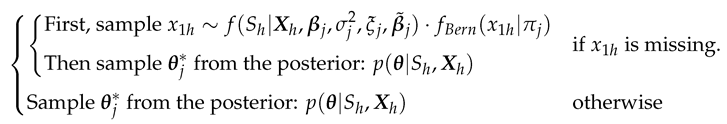
a): Imputation: The missing covariate impacts on the parameter - $θ, w$ - update. For $w_{j}$ , only the observations $S_{h}$ without the missing covariate are used to update. If the cluster does not have any observations with complete data for that covariate, then a draw from the prior distribution would be used to update. For $θ_{j}$ , however, we must first impute values for the missing covariates $x_{1 h}$ for all observations $S_{h}$ within the cluster. Since having already defined a full joint model - $f (S_{h} | X_{h}, θ_{j}) \cdot f (X_{h} | w_{j})$ - in Section 3.2, we can obtain draws for the MAR covariate $x_{1 h}$ from the imputation model such as $f_{B e r n} (x_{1 h} | S_{h}, θ_{j}, w_{j}) \propto f (S_{h} | X_{h}, β_{j}, σ_{j}^{2}, ξ_{j}) \cdot f_{B e r n} (x_{1 h} | π_{j})$ at each iteration of the Gibbs sampler. The imputation process is briefly illustrated in Figure 3. Once all missing data in all covariates has been imputed, then we can sample from the posterior for $θ$ and the parameters of each cluster $β_{j}, σ_{j}^{2}$ are re-calculated. After this cycle is complete, the imputed data is discarded and the same imputation steps are repeated every iteration.
b): Re-clustering: To determine each cluster probability after the imputations, the algorithm re-defines the two main components for the cluster probability calculation - 1) covariate model, 2) outcome model. For the covariate model $f (X_{h} | w_{j})$ , we set this equal to the density functions of only those covariates with complete data for observation h. Assuming that $X_{h} = {x_{1 h}, x_{2 h}}$ , and the covariate $x_{1}$ is missing for observation h, then we drop $x_{1 h}$ and only use $x_{2 h}$ in the covariate model,

$f (X_{h} | w_{j}) = f_{N} (x_{2 h} | w_{2 j})$

(8)

This is the refined covariate model for the cluster j with the observation h where the data in $x_{1}$ is not available. For the outcome model $f (S_{h} | X_{h}, θ_{j})$ , the algorithm simply takes the imputation model for each cluster and integrates them out the covariates with missing data. This reduces the degree of variances introduced by the imputations. In our case, as covariate $x_{1}$ is missing for observation h, this missing covariate can be removed from the $X_{h}$ term that is being conditioned on. Therefore, the refined outcome model is

$f (S_{h} | x_{2 h}, θ_{j}) \propto \int f (S_{h} | X_{h}, θ_{j}) \cdot f_{B e r n} (x_{1 h} | w_{1 j}) d x_{1 h}$

(9)

A similar process is conducted for each observation with missing data and each combination of missing covariates. Hence, using Equation (8,9), the cluster probabilities and the predictive distribution can be obtained as illustrated in Step III in Figure 4.
c): Parameter update: The cluster probability computation is followed by the parameter re-estimation for each cluster, which is illustrated via the diagram in Figure 5. This is the same idea as what we have discussed about the parameter - $θ, w$ - update in Figure 2.

4. Bayesian Inference for $S_{h} | X_{h}$ with MAR Covariate

The efficient simulation for the model parameters -

θ : {β, σ^{2}, ξ \tilde{β}}, w : {π, μ, τ^{2}}

, and

α

- requires the proper parameterization in the parameter models - prior parameter model and posterior parameter model. The accurate estimations of cluster probabilities rely on the legitimate development of data models - outcome model and covariate model - and the model parameter simulation results that govern the data model behaviors. This section is centered on the novel development of parameter and data models, providing the details of the DPM implementation integrated with the MAR imputation strategy.

4.1. Parameter Models and MAR Covariate

Our study is based on a three-level hierarchical structure: the first level regards the data models such as the log skew-normal outcome model and the Bernoulli, Gaussian covariate models, the second level involves the parameter models such as

p (θ | S_{h}, X_{h}), p (w | X_{h})

to explain the data, and the third level is developed from the generalized regression to explain the parameters or the related hyperparameters such as

a_{0}, b_{0}, ν_{0}, c_{0}, d_{0}, μ_{0}, τ_{0}^{2}, e_{0}, γ_{0}, g_{0}

and

h_{0}

to set a probabilistic distribution on the parameter vectors

θ = {β, σ^{2}, ξ, \tilde{β}}, w = {π, μ, τ^{2}}

. See Variable Definition for further information on the variables. Given the model definition in Equation (1), we consider a set of conjugate parameter models due to its computational advantages [21]. For

S_{h} \sim δ (X_{h}^{T} {\tilde{β}}_{j}) 1 (S_{h} = 0) + [1 - δ (X_{h}^{T} {\tilde{β}}_{j})] L o g S N (X_{h}^{T} β_{j}, σ_{j}^{2}, ξ_{j})

x_{1} \sim B e r n (π_{j})

, and

x_{2} \sim N (μ_{j}, τ_{j}^{2})

, the prior models come in

\begin{matrix} p_{0} (σ_{j}^{2} | a_{0}, b_{0}) : & InvGa (a_{0}, b_{0}), & p_{0} (β_{j} | β_{0}, Σ_{0}) : & MVN (β_{0}, σ_{j}^{2} Σ_{0}), & p_{0} (ξ_{j} | ν_{0}) : T (ν_{0}) \\ p_{0} ({\tilde{β}}_{j} | {\tilde{β}}_{0}, {\tilde{Σ}}_{0}) : & MVN ({\tilde{β}}_{0}, {\tilde{Σ}}_{0}), & p_{0} (π_{j} | c_{0}, d_{0}) : & Beta (c_{0}, d_{0}), & p_{0} (μ_{j} | μ_{0}, τ_{0}^{2}) : N (μ_{0}, τ_{j}^{2}), \\ p_{0} (τ_{j}^{2} | e_{0}, γ_{0}) : & InvGa (e_{0}, γ_{0}), & p_{0} (α | g_{0}, h_{0}) : & Ga (g_{0}, h_{0}) \end{matrix}

and their corresponding kernels chosen in this study are listed in Appendix A.1. Accordingly, the Dirichlet process prior (probability measure)

G_{0}

in our case can be defined as

G_{0} = MVN (β_{0}, Σ_{0}) \times InvGa (a_{0}, b_{0}) \times T (ν_{0}) \times MVN ({\tilde{β}}_{0}, {\tilde{Σ}}_{0}) \times Beta (c_{0}, d_{0}) \times N (μ_{0}, τ_{j}^{2}) \times InvGa (e_{0}, γ_{0}) \times Ga (g_{0}, h_{0})

. With a feed of the observed data inputs -

(S_{h}, x_{1 h}, x_{2 h})

-, the prior models for each cluster j described above will be updated into the following posterior models analytically apart from

θ_{j} = {β_{j}, σ_{j}^{2}, ξ_{j}, {\tilde{β}}_{j}}

\begin{matrix} p (π_{j} | c_{0}, d_{0}, S, x_{1}) : Beta (c_{n e w}, d_{n e w}) \\ p (μ_{j} | μ_{0}, τ_{0}^{2}, S, x_{2}) : N (μ_{n e w}, τ_{n e w}^{2}), p (τ_{j}^{2} | e_{0}, γ_{0}, S, x_{2}) : InvGa (e_{n e w}, γ_{n e w}) \\ p (α | g_{0}, h_{0}, h, J, η, π_{η}) : π_{η} Ga (g_{0} + J, h_{0} - l o g (η)) + (1 - π_{η}) Ga (g_{0} + J - 1, h_{0} - l o g (η)) \end{matrix}

(10)

and their corresponding parameterizations are elaborated in Appendix A.2. Note that the value of the precision parameter

α

relies on the total cluster number J, thus does not vary by the cluster membership j, and its derivation of the posterior parameterization is not subject to the Bayesian conjugacy. Hence, we instead adapt the form of the posterior density for the

α

suggested by Escobar and West (1995) [22], and its derivation is shown in Appendix C.1. As for

θ_{j} = {β_{j}, σ_{j}^{2}, ξ_{j}, {\tilde{β}}_{j}}

, there are no conjugate priors available for log skew-normal likelihood, but their posterior samples can be secured by the conventional metropolis hastings described in Algorithm (A2) in Appendix A.

Considering that

x_{1}

has missing data, although the parameterizations of the posterior densities for the covariate parameter model of

w

and the precision

α

listed in Equation (10) are not affected, any outcome data of

S_{h}

with missingness should be dropped; therefore,

n_{j}

and

x_{1}

are defined with the only observations in cluster j that are not missing. This imputation example is provided in Appendix C.2. For the outcome parameter model of

θ_{j}

, the missing covariate

x_{1}

must be imputed before its posterior computation shown in Algorithm (A2). Once the parameters are updated with the imputation, the data models can be constructed as described in Equation (8,9).

4.2. Data Models and MAR Covariate

Data models are the main components for cluster probability computations depicted in Figure 2. As with the development of parameter models, the covariate data model of

X

ignores the observations with missingness while the outcome data model of

S_{h}

requires to complete the covariates beforehand. However, the formulation of their densities can be more complex due to the marginalization process with respect to the missing covariate. In addition, as discussed in Section 3.2, the data model development is bound by the types of clusters such as discrete clusters

f (S_{h} | X_{h}, θ_{j}), f (X_{h} | w_{j})

and continuous clusters

f_{0} (S_{h} | X_{h}), f_{0} (X_{h})

a)

covariate model for the discrete cluster: $f (X_{h} | w_{j})$

Focusing on the scenario that

x_{1}

is binary,

x_{2}

is Gaussian, and the only covariate with missingness is

x_{1 h}

, we simply drop the covariate

x_{1 h}

to develop the covariate model for the discrete cluster. For instance, when computing the covariate probability term for hth observation in j cluster, the covariate model

f (x_{1 h}, x_{2 h} | π_{j}, μ_{j}, τ_{j}^{2})

simply becomes

f (x_{2 h} | μ_{j}, τ_{j}^{2})

due to the missingness of

x_{1 h}

. As we have

x_{2}

that is assumed to be normally distributed as defined in Equation (1), its probability term is

f (x_{2 h} | μ_{j}, τ_{j}^{2}) = \frac{1}{\sqrt{2 π τ_{j}^{2}}} exp {\frac{- {(x_{2 h} - μ_{j})}^{2}}{2 τ_{j}^{2}}}

(11)

instead of

f (x_{1 h}, x_{2 h} | π_{j}, μ_{j}, τ_{j}^{2}) = π_{j}^{x_{1 h}} {(1 - π_{j})}^{1 - x_{1 h}} \cdot \frac{1}{\sqrt{2 π τ_{j}^{2}}} exp {\frac{- {(x_{2 h} - μ_{j})}^{2}}{2 τ_{j}^{2}}}

b)

covariate model for the continuous cluster: $f_{0} (X_{h})$

If the binary covariate

x_{1 h}

is missing, by the same logic, we drop the covariate

x_{1 h}

for the continuous cluster; however, using Equation (4), the covariate model for the continuous cluster integrates out the relevant parameters simulated from the Dirichlet process prior

G_{0}

as follows:

\begin{matrix} f_{0} (x_{2 h}) = \int f (x_{2 h} & | μ, τ^{2}) d G_{0} (μ, τ^{2}) = \int f (x_{2 h} | μ, τ^{2}) \cdot p (μ | τ^{2}) \cdot p (τ^{2}) d μ d τ^{2} \\ = \frac{γ_{0}^{e_{0}} Γ (e_{0} + 1 / 2)}{2 \sqrt{π} Γ (e_{0})} {(γ_{0} + \frac{{(x_{2 h} - μ_{0})}^{2}}{4})}^{- (e_{0} + 1 / 2)} \end{matrix}

(12)

instead of

\begin{matrix} f_{0} ( & x_{1 h}, x_{2 h}) = \int f (x_{1 h}, x_{2 h} | π, μ, τ^{2}) \cdot p (π) \cdot p (μ | τ^{2}) \cdot p (τ^{2}) d π d μ d τ^{2} \\ = \frac{B (x_{1 h} + c_{0}, 1 - x_{1 h} + d_{0})}{B (c_{0}, d_{0})} \cdot \frac{γ_{0}^{e_{0}} Γ (e_{0} + 1 / 2)}{2 \sqrt{π} Γ (e_{0})} {(γ_{0} + \frac{{(x_{2 h} - μ_{0})}^{2}}{4})}^{- (e_{0} + 1 / 2)} \end{matrix}

The derivation of the distributions above is provided in Appendix C.3.

c)

outcome model for the discrete cluster: $f (S_{h} | X_{h}, θ_{j})$

In developing the outcome model, as with the parameter model case discussed in Section 4.1 and Appendix C.2, it should be ensured that the covariate is complete beforehand. With all missing data in

x_{1 h}

imputed, the outcome model for the discrete cluster is obtained by marginalizing the joint -

f (S_{h}, x_{1 h} | x_{2 h}, θ_{j}, π_{j})

- out the MAR covariate

x_{1 h}

, which is a log skew-normal mixture as follows:

\begin{matrix} f (S_{h} | x_{2 h}, β_{j}, σ_{j}^{2}, ξ_{j}, {\tilde{β}}_{j}) = \sum_{x_{1 h} = 0}^{1} f (S_{h} | x_{1 h}, x_{2 h}, β_{j}, σ_{j}^{2}, ξ_{j}, {\tilde{β}}_{j}) \cdot f (x_{1 h} | π_{j}) \\ = f (S_{h}, x_{1 h} = 1 | x_{2 h}, β_{j}, σ_{j}^{2}, ξ_{j}, {\tilde{β}}_{j}, π_{j}) + f (S_{h}, x_{1 h} = 0 | x_{2 h}, β_{j}, σ_{j}^{2}, ξ_{j}, {\tilde{β}}_{j}, π_{j}) \\ = δ (X_{h}^{T} {\tilde{β}}_{j}) 1 (S_{h} = 0) + [1 - δ (X_{h}^{T} {\tilde{β}}_{j})] \cdot \frac{2}{σ_{j} S_{h}} \\ \cdot ϕ (\frac{log S_{h} - (β_{j 0} + β_{j 1} + β_{j 2} x_{2 h})}{σ_{j}}) \cdot Φ (ξ_{j} \frac{log S_{h} - (β_{j 0} + β_{j 1} + β_{j 2} x_{2 h})}{σ_{j}}) π_{j} \\ + δ (X_{h}^{T} {\tilde{β}}_{j}) 1 (S_{h} = 0) + [1 - δ (X_{h}^{T} {\tilde{β}}_{j})] \cdot \frac{2}{σ_{j} S_{h}} \\ \cdot ϕ (\frac{log S_{h} - (β_{j 0} + β_{j 2} x_{2 h})}{σ_{j}}) \cdot Φ (ξ_{j} \frac{log S_{h} - (β_{j 0} + β_{j 2} x_{2 h})}{σ_{j}}) \cdot (1 - π_{j}) \end{matrix}

(13)

instead of

\begin{matrix} f (S_{h} | x_{1 h}, x_{2 h}, β_{j}, σ_{j}^{2}, ξ_{j}, {\tilde{β}}_{j}) \\ = δ (X_{h}^{T} {\tilde{β}}_{j}) 1 (S_{h} = 0) + [1 - δ (X_{h}^{T} {\tilde{β}}_{j})] \cdot \frac{2}{σ_{j} S_{h}} \\ \cdot ϕ (\frac{log S_{h} - (β_{j 0} + β_{j 1} x_{1 h} + β_{j 2} x_{2 h})}{σ_{j}}) \cdot Φ (ξ_{j} \frac{log S_{h} - (β_{j 0} + β_{j 1} x_{1 h} + β_{j 2} x_{2 h})}{σ_{j}}) \end{matrix}

d)

outcome model for the continuous cluster: $f_{0} (S_{h} | X_{h})$

Once a missing covariate

x_{1}

is fully imputed and the outcome model is marginalized out conditioned to the MAR covariate

x_{1 h}

, the outcome model

f_{0} (S_{h} | x_{2 h})

for the continuous cluster can also be computed by integrating out the relevant parameters, using Equation (4).

f_{0} (S_{h} | x_{2 h}) = \int f (S_{h} | x_{2 h}, β, σ^{2}, ξ, \tilde{β}) \cdot p (β) \cdot p (σ^{2}) \cdot p (ξ) \cdot p (\tilde{β}) d β d σ^{2} d ξ d \tilde{β}

(14)

However, it can be too complicated to compute its form analytically. Instead, we can integrate the joint model out the parameters, using Monte Carlo integration. For example, we can do the following for each

h = 1, \dots, H

(i): Sample $β, σ^{2}, ξ, \tilde{β}$ from the DP prior densities $G_{0}$ specified previously.
(ii): Plug in these samples into $f (S_{h} | x_{2 h}, β, σ^{2}, ξ, \tilde{β}) \cdot p (β) \cdot p (σ^{2}) \cdot p (ξ) \cdot p (\tilde{β})$ .
(iii): Repeat the above steps many times, recording each output.
(iv): Divide the sum of all output values by the number of Monte Carlo samples, which will be the approximate integral.

4.3. Gibbs Sampler Modification for MAR Covariate

We have examined the parameter models and data models to update the parameters of the DPM based on probabilistically imputed values of the MAR covariate. Now we set out some modifications of the DPM and let the Gibbs sampler in Algorithm (A2) in Appendix B. address the MAR covariate of

x_{1}

. The Gibbs sampler will alternate between imputing missing data and drawing parameters until it reaches a stationary distribution of the parameters. We elaborate below on the modifications that fit into Algorithm (A2) to update the clustering scenarios and the posterior cluster parameters properly.

a): In line 6, with the presence of missing covariate $x_{1 h}$ , the modification of the cluster probability for the observation $(S_{h}, x_{1 h}, x_{2 h})$ that belongs to the discrete cluster j can be made as follows,

$P (s_{h} = j) = p (s_{h} | s_{- h}) \cdot f (x_{2 h} | μ_{j}, τ_{j}^{2}) \cdot f (S_{h} | x_{2 h}, β_{j}, σ_{j}^{2}, ξ_{j}, {\tilde{β}}_{j})$

where $f (x_{2 h} | μ_{j}, τ_{j}^{2})$ is from Equation (11), and $f (S_{h} | x_{2 h}, β_{j}, σ_{j}^{2}, ξ_{j}, {\tilde{β}}_{j})$ is from Equation (13).
b): In line 9, with the presence of missing covariate $x_{1 h}$ , the modification of the cluster probability for the observation $(S_{h}, x_{1 h}, x_{2 h})$ that belongs to the continuous cluster $J + 1$ can be made as follows,

$P (s_{h} = J + 1) = p (s_{h} | s_{- h}) \cdot f_{0} (x_{2 h}) \cdot f_{0} (S_{h} | x_{2 h})$

where $f_{0} (x_{2 h})$ is from Equation (12), and $f_{0} (S_{h} | x_{2 h})$ is from Equation (14).
c): In line 22, with the presence of missing covariate $x_{1 h}$ , the imputation should be made before simulating the parameter $θ_{j}^{*}$ as follows,

The imputation model formulation in the above has been discussed in Section 3.4.

Again, these modifications allow to draw missing covariate values from the conditional posterior density at each iteration, using the Metropolis-Hastings with a random walk.

5. Empirical Study

5.1. Data

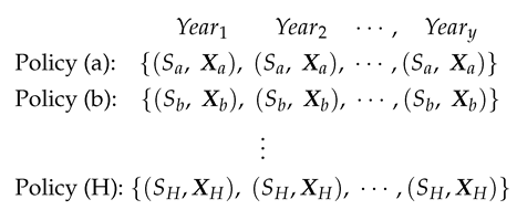
The performance of our DPM framework is assessed based on two insurance datasets. They highlight data difficulties such as unobservable heterogeneity in an outcome variable and MAR covariates. For simplicity, in each dataset, we only consider two covariates - one binary and one continuous - to explain its loss information (outcome variable). In this study, all computations on these two datasets are performed in the same data format:

The first dataset is PnCdemand, which is about the international property and liability insurance demand of 22 countries over 7 years from 1987 to 1993. Secondly, we use a dataset drawn from the Wisconsin Local Government Property Insurance Fund (LGPIF) with information about the insurance coverage for government building units in Wisconsin for years from 2006 to 2010. The first one - PnCdemand - can be obtained from the R package CASdatasets. The dataset is relatively small as it has

H = 240

cases with an outcome variable GenLiab: the individual loss amount under the policies of general insurance for each case. As for covariates, we consider one indicator variable of the statutory law system (LegalSyst:1 or 0) and one continuous variable that measures a risk aversion rate (RiskAversion) for each area. For additional background on this dataset, see Browne et al. (2000) [23]. In the LGPIF dataset, the insurance coverage samples for the government properties from

H = 5660

policies are provided. The outcome variable is the sum of all types of losses (Total Losses) for each policy. Only the covariates - LnCoverage, Fire5 - are considered in our study. Fire5 is a binary covariate that indicates fire-protection levels while LnCoverage is a continuous covariate that informs a total coverage amount in a logarithmic scale. For further details, see Quan et al. [24].

Histograms of the losses of the two datasets are exhibited in Figure 6. Due to the significant skewness, the loss data are log-transformed to attain Gaussianity. As shown in the histograms, each distribution displays different characteristics in regard to skewness, modality, excess of zeros, etc. Note that the zero-inflated outcome variable in LGPIF data (b1, b2 in Figure 6) requires a two-part modeling technique that distinguishes the probabilities of the outcome being zero and positive.

5.2. Three Competitor Models and Evaluation

Our DPM framework is compared to other commonly used actuarial models in practice. We employ three predictive models as benchmarks - namely, a generalized linear mixture model (GLM), multivariate adaptive regression spline (MARS), and generalized additive model (GAM). In each dataset, we assume different distributions for the outcome variables, and thus the three benchmark models are built upon the different outcome data models. For example, the PnCdemand dataset (a1,a2) that appeared in Figure 6, has a high frequency of small losses without zero values, hence it is safe to use a gamma mixture to explain the outcome data. As for the LGPIF data (b1,b2) in Figure 6, we consider the outcome data model based on a Tweedie distribution to accommodate the zero-inflated loss data. The benchmark models are implemented in R with the mgcv, splines, and mice packages.

All four models are trained, and investigations are performed in terms of model fit, prediction accuracy, and the conditional tail expectation (CTE) of the predictive distribution. Note that the goodness of fit value for a DPM is not available in Table 1,Table 2. Teh (2010) [25] argues that the goodness of fit evaluation for a DPM is unnecessary as underfitting is mitigated by the unbounded complexity of a DPM while overfitting is alleviated by the approximation of posterior densities over each parameter in a DPM. Gelman et al. (2007) [26] point out Posterior predictive check, which compares the simulated data under the fitted DPM to the observed data, can be useful in studying model adequacy, but its usage cannot be for model comparison. Therefore, the goodness of fit is only compared between the rival models. For the evaluation of prediction performance, the sum of square prediction error (SSPE) and sum of square absolute error (SAPE) are used.

5.3. Result 01. International General Insurance Liability Data

For this dataset, a training set of response and covariates pair

(Y, X)

with n = 160 records, and a test set of response and covariates pair

(Y^{'}, X^{'})

with m = 80 records are constructed. We implement the following DPM:

\begin{matrix} Y_{h} | x_{1}, x_{2}, β_{j}, σ_{j}^{2} & \sim L o g N (X^{T} β_{j}, σ_{j}^{2}) \\ x_{1} | π_{j} & \sim B e r n (π_{j}) \\ x_{2} | μ_{j}, τ_{j}^{2} & \sim N (μ_{j}, τ_{j}^{2}) \\ {θ_{j}, w_{j}} & \sim G \\ G & \sim D P (α, G_{0}) \end{matrix}

A log-normal likelihood is chosen to accommodate the individual loss

Y_{h}

:GenLiab for a policy h. The covariate

x_{2}

:RiskAversion is subject to missingness, and found to depend on

Y_{h}

(a MAR case). This is addressed by the internalized imputation process as discussed in Figure 3. The posterior parameters of

θ_{j}, w_{j}

are estimated with our DPM Gibbs sampler presented in Algorithm (A2). The algorithm runs 10,000 iterations until convergence, and the resulting scenarios of clustering mixture are shown in Figure 7. The plot reveals the overlays of predictive densities on the log scale from the last 100 iterations that are tied to convergence.

Figure 8 lists the classical data imputation process - Multivariate Imputation Chained Equation (MICE) - and predictive densities produced from our rival models - GLM, GAM, MARS. The MICE runs multiple imputation chains, and selects the imputation values from the final iteration. This process results in multiple candidate datasets. The trace plots (a1,a2) monitor the imputation mean and variance for the missing values in the dataset. In the covariate distribution plot (a3), the density of the observed covariate shown in blue is compared with the ones of the imputed covariate for each imputed dataset shown in red. The parameter inferences for the rival models are performed based on the imputed datasets tied to convergence [27]. The gamma distribution is chosen to fit the rival models as the

Y_{h}

is continuous and positively skewed with a constant coefficient of variation. The gamma-based predictive density plots (b1,b2,b3) estimated with GLM, GAM, MARS look similar, showing unusual bumps near the right tail.

In Figure 9, a histogram of the outcome data in the test set is displayed. The posterior mean densities for out-of-sample predictions produced with our DPM along with the rival models’ density estimates are overlaid on the histogram. Judging from the plot, one can say that our DPM model generates the best approximation. While the rival models generate smooth, mounded curves to make predictions, our DPM captures all possible peaks and bumps, which is closer to the actual situation. According to Table 1, the rival models produce slightly higher SAPEs, but lower SSPEs, compared to our proposed DPM. As SAPE weights all the individual differences equally, we can assume that the rival models tend to give too much focus on the most probable data points and miss some outliers. This is mainly due to the insufficient sample size. However, our DPM has good performance under small sample sizes when there is sufficient prior knowledge available. From the perspective of CTE, Table 1 shows that our DPM proposes a heavier tail than other rival models, which reflects that our DPM captures more uncertainties given the small sample size.

5.4. Result 02. LGPIF Data

For this dataset, a training set of response and covariates pair

(S, X)

with n = 4529 records, and a test set of response and covariates pair

(S^{'}, X^{'})

with m = 1110 records are constructed. We implement the following DPM:

\begin{matrix} S_{h} | x_{1}, & x_{2}, β_{j}, σ_{j}^{2}, ξ_{j}, {\tilde{β}}_{j} \\ \sim δ (X^{T} {\tilde{β}}_{j}) 1 (S_{h} = 0) + [1 - δ (X^{T} {\tilde{β}}_{j})] L o g S N (X^{T} β_{j}, σ_{j}^{2}, ξ_{j}) \\ x_{1} | π_{j} & \sim B e r n (π_{j}) \\ x_{2} | μ_{j}, τ_{j}^{2} & \sim N (μ_{j}, τ_{j}^{2}) \\ {θ_{j}, w_{j}} & \sim G \\ G & \sim D P (α, G_{0}) \end{matrix}

As the outcome

S_{h}

:Total Losses for a policy h in this dataset is considered to be distributed with the sum of log-normal densities, a log skew-normal likelihood is chosen to approximate this convolution [7]. The covariate

x_{1}

:Fire5 is subject to missingness under MAR, and the internalized imputation process illustrated in Figure 3 resolves this issue without creating imputed datasets. As the outcome

S_{h}

exhibits zero inflation, we employ a two-part model, using a sigmoid and indicator function. Our DPM Gibbs sampler described in Algorithm (A2) produces the posterior parameters of

θ_{j}, w_{j}

with 10,000 iterations until convergence. Figure 10 reveals the resulting scenarios of clustering mixture. In the plot, there are 100 predictive densities suggested by our DPM, each of which stands for the convergence of the estimation results.

The output of the MICE and the resulting predictive densities from the rival models are displayed in Figure 11. The rival models are built upon a Tweedie distribution due to its ability to account for a large number of zero losses, and the flexibility to capture the unique loss patterns of the different classes of policyholders. According to the plot, all three rival models reasonably capture zero inflation, but the GAM tends to suggest more bumps that indicate a need for further assessment of the prediction uncertainty.

The overall out-of-sample prediction comparison is made in the histogram overlayed with predictive density curves generated from the four models in Figure 12. From the plot, it is apparent that the posterior predictive density proposed by our DPM best explains the new samples while other rival models keep producing multiple peaks. The prediction performance of our DPM is confirmed by the smallest SSPE and SAPE in Table 2. In terms of CTE, all three rival models suggest a similar level of tailedness, reflecting the knowledge obtained from the observed data. However, our DPM goes beyond this and proposes a much heavier tail. This is because our DPM accommodates the presence of outliers and shapes the tail behavior based on the combined knowledge of prior parameters and the observations available.

6. Discussion

This paper proposes a novel DPM framework for actuarial practice to model total losses with the incorporation of MAR covariates. Both log-normal and log skew-normal DPM present overall good empirical performances in capturing the shape of the distribution, out-of-sample prediction, and the estimation of the tailedness. This suggests that it is worth considering our DPM framework in order to avoid various model risks or biases in insurance claim analysis.

6.1. Research Questions

Regarding RQ1, we propose a DPM framework to address the within-cluster heterogeneity emerging from the inclusion of covariates. By allowing for an infinite number of clustering scenarios determined by the observations as well as prior knowledge, our DPM outperforms the rival methods in drawing the lines for the cluster membership. This can be assessed by examining the homogeneity of the resulting clusters. In our case, we fit cluster-wise GLMs (based on Gamma and Tweedie) to the data points within each resulting cluster to compare the goodness-of-fit, and the consistent AICs across all clusters endorse the benefits of the DPM. Similarly, our rival methods such as GAM or MARS can capture heterogeneity by using customized smooth functions across different subsets of the data, but we observe some statistically insignificant smooth terms, indicating the presence of heterogeneity in the cluster.

In terms of RQ2, we suggest incorporating the imputation steps into the parameter and cluster membership update process in the DPM Gibbs sampler by leveraging the joint distribution of the observed outcomes and missing covariates. This approach allows the imputed values to be consistent with the observed data, preserving the correlation structure within the dataset. In order to make a comparison of our approach with an existing alternative, we additionally employ a chained equation technique. The multiple sets of imputed values simulated from both approaches are investigated, and the result shows that our DPM Gibbs sampler does not represent a significant improvement over the chained equation because their average estimates of the imputed values are closer to each other. However, we feel that this result is mainly due to the relatively low dimensionality of the datasets we use and their simple data structure. The specific characteristics or dependencies in the data and the complexity of the missing patterns would give different results in practice.

As for RQ3, we fit a log skew-normal density to the aggregate loss outcomes. In order to assess its performance, one can consider Minimax approximation, Least squares approximation, Log shifted gamma approximation, etc. as the competitors. Li (2008) [7] provides a useful comparison between these competitors by overlaying the cumulative density curves for each technique, but its experiments are grounded on the simulated log-normal data with the pre-defined parameters and assumptions, which cannot be easily controlled in real-world scenarios. Therefore, we feel that the choice of the best approximation technique should be made based on the identification of the specific characteristics of the dataset. In our case, each summand in our dataset is significantly different from each other in magnitudes (the Minimax is inappropriate) and LGPIF data has a large volume of data smaller than 5 (the Log shifted gamma is inappropriate); therefore, we choose a log skew-normal density that is relatively simple while giving an accurate approximation at the lower region of the distribution.

6.2. Future Work

There are several concerns with our log skew-normal DPM framework.

(a): Dimensionality: First, in our analysis, we only use two covariates (binary and continuous) for simplicity, hence more complex data should be considered. As the number of covariates grows, the likelihood components (covariate models) to describe the covariates grow, which results in the shrinking of the cluster weights. Therefore, using more covariates might enhance the level of sensitivity and accuracy in the creation of cluster memberships. However, it can also introduce more noise or hidden structures that render the resulting predictive distributions unstable. In this sense, further research on the problem of high dimensional covariates in the DPM framework would be worthwhile.
(b): Measurement error: Second, although our focus in this article is MAR covariate, mismeasured covariate is an equally significant challenge that impairs the proper model development in insurance practice. For example, Aggarwal et al. (2016) [28] point out that “model risk" mainly arises due to missingness and measurement error in variables, leading to flawed risk assessments and decision-making. Thus, further investigation is necessary to explore the specialized construction of the DPM Gibbs sampler for mismeasured covariates, aiming to prevent the issue of model risk.
(c): Sum of log skew-normal: Third, as an extension to the approximation of total losses $S_{h}$ (the sum of individual losses) for a policy, we recommend researching into ways to approximate the sum of total losses $\tilde{S}$ across entire policies. In other words, we pose the question of “how to approximate the sum of log skew-normal random variables". From the perspective of an executive or an entrepreneur whose concern is the total cash flow of the firm, nothing might be more important than the accurate estimation of the sum of total losses in order to identify the insolvency risk or to make important business decisions.
(d): Scalability: Lastly, we suggest investigating the scalability of the posterior simulation by our DPM Gibbs sampler. As shown in our empirical study on the PnCdemand dataset, our DPM framework produces reliable estimates with relatively small sample sizes ( $n \leq 160$ ). This is because our DPM framework actively utilizes significant prior knowledge in posterior inference rather than heavily relying on the actual features of the data. In the result from the LGPIF dataset, our DPM exhibits stable performance at sample size $n = 4529$ as well. However, a sample size of over 10000 is not explored in this paper. With increasing amounts of data, our DPM framework raises a question of computational efficiency due to the growing demand for computational resources or degradation in performance [29]. This is an important consideration, especially in scenarios where the insurance loss information is expected to grow over time.

7. Variable Definitions

The following variables and functions are used in this manuscript:

$i = 1, \dots, N_{h}$	observation index i in policy h.
$h = 1, \dots, H$	policy index h with sample (policy) size H.
$j = 1, \dots, J$	cluster index for J clusters.
$s_{h}$	cluster index $j = 1, \dots, J$ for observation h.
$n_{j}$	number of observations in cluster j.
$n_{j}^{- h}$	number of observations in cluster j where observation h removed from.
$Y_{i h}$	individual loss i in a policy observation h.
$S_{h}$	outcome variable which is a $Σ Y_{i h}$ in a policy observation h.
$\tilde{S}$	outcome variable which is a $Σ S_{h}$ across entire policies
$X_{h}$	vector of covariates (including $x_{1}, x_{2}$ ) for observation h.
$x_{1}$	vector of covariate (Fire5).
$x_{2}$	vector of covariate (Ln(coverage)).
$x_{1}$	individual value of covariate (Fire5).
$x_{2}$	individual value of covariate (Ln(coverage)).
$p_{0} (\cdot)$	parameter model (for prior).
$p (\cdot)$	parameter model (for posterior).
$f_{0} (\cdot)$	data model (for continuous cluster).
$f (\cdot)$	data model (for discrete cluster).
$δ (\cdot)$	logistic sigmoid function - expit(·) - to allow for a positive probability of the zero outcome.
$θ_{j}$	set of parameters - $β, σ^{2}, ξ$ - associated with the $f (Σ Y \| X)$ for j cluster.
$w_{j}$	set of parameters - $π, μ, τ$ - associated with the $f (X)$ for j cluster.
$ω_{j}$	cluster weights (mixing coefficient) for j cluster.
$β_{0}, Σ_{0}$	vector of initial regression coefficients and variance-covariance matrix, i.e. ${\hat{σ}}^{2} {(X^{T} X)}^{- 1} = X^{T} X {(Σ Y - Σ \hat{Y})}^{T} (Σ Y - Σ \hat{Y}) / (n - p)$ obtained from the baseline multivariate Gamma regression of $Σ \hat{Y} > 0$ .
$β_{j}$	regression coefficient vector for a mean outcome estimation.
$σ_{j}^{2}$	cluster-wise variation value for the outcome.
$ξ_{j}$	skewness parameter for log skew-normal outcome.
${\tilde{β}}_{0}, {\tilde{Σ}}_{0}$	vector of initial regression coefficients and variance-covariance matrix obtained from the baseline multivariate logistic regression of $Σ \hat{Y} = 0$ .
${\tilde{β}}_{j}$	regression coefficient vector for a logistic function to handle zero outcomes.
$π_{j}$	proportion parameter for Bernoulli covariate.
$μ_{j}, τ_{j}$	location and spread parameter for Gaussian covariate.
$α$	precision parameter that controls the variance of the clustering simulation. For instance, a larger $α$ allows to select more clusters.
$G_{0}$	prior joint distribution for all parameters in the DPM - $β, σ^{2}, ξ, π, μ, τ$ , and $α$ . It allows all continuous, integrable distributions to be supported while retaining theoretical properties and computational tractability such as asymptotic consistency, efficient posterior estimation, etc.
$a_{0}, b_{0}$	hyperparameters for Inverse Gamma density of $σ_{j}^{2}$ .
$c_{0}, d_{0}$	hyperparameters for Beta density of $π_{j}$ .
$ν_{0}$	hyperparameters for Student’s t density of $ξ_{j}$ .
$μ_{0}, τ_{0}^{2}$	hyperparameters for Gaussian density of $μ_{j}$ .
$e_{0}, γ_{0}$	hyperparameters for Inverse Gamma density of $τ_{j}^{2}$ .
$g_{0}, h_{0}$	hyperparameters for Gamma density of $α$ .
$η$	random probability value for Gamma mixture density of the posterior on $α$ .
$π_{η}$	mixing coefficient for Gamma mixture density of the posterior on $α$ .

Author Contributions

All authors contributed substantially to this work - Conceptualization, Kim.M.; Methodology, Kim.M., Lindberg.D., Bezbradica.M. and Crane.M.; Software, Kim.M., Lindberg.D.; Validation, Kim.M., Bezbradica.M and Crane.M.; Formal analysis, Kim.M.; Investigation, Kim.M., Bezbradica.M and Crane.M.; Resources, Kim.M.; Data curation, Kim.M.; Writing—original draft preparation, Kim.M.; Writing—review and editing, Kim.M., Bezbradica.M and Crane.M.; Visualization, Kim.M.; Supervision, Bezbradica.M and Crane.M.; Project administration, Bezbradica.M and Crane.M.; Funding acquisition, Crane.M. All authors have read and agreed to the published version of the manuscript.

Data Availability Statement

Data and implementation details are available at https://github.com/mainkoon81/Paper2-Nonparametric-Bayesian-Approach01 (accessed on 25 May 2023).

Acknowledgments

For this research, the authors wish to acknowledge the support from the Science Foundation Ireland under Grant Agreement No.13/RC/2106 P2 at the ADAPT SFI Research Centre at DCU. ADAPT, the SFI Research Centre for AI-Driven Digital Content Technology, is funded by the Science Foundation Ireland through the SFI Research Centres Programme.

Conflicts of Interest

The authors declare no conflict of interest.

Appendix A Parameter Knowledge

Appendix A.1. Prior Kernel for Distributions of Outcome, Covariates, and Precision

\begin{matrix} p_{0} (β_{j} | β_{0}, Σ_{0}) & : MVN {(β_{0}, σ_{j}^{2} Σ_{0})}^{*} \propto e^{{{(β_{j} - β_{0})}^{T} Σ_{0}^{- 1} (β_{j} - β_{0})}}, p_{0} (σ_{j}^{2} | a_{0}, b_{0}) : InvGa (a_{0}, b_{0}) \propto {(σ_{j}^{2})}^{- (a_{0} + 1)} \cdot e^{- b_{0} / σ_{j}^{2}} \\ p_{0} (ξ_{j} | ν_{0}) & : T (ν_{0}) \propto {(\frac{ξ_{j}^{2}}{ν_{0}} + 1)}^{- (ν_{0} + 1) / 2}, p_{0} ({\tilde{β}}_{j} | {\tilde{β}}_{0}, {\tilde{Σ}}_{0}) : MVN {({\tilde{β}}_{0}, {\tilde{Σ}}_{0})}^{*} \propto e^{{{({\tilde{β}}_{j} - {\tilde{β}}_{0})}^{T} {\tilde{Σ}}_{0}^{- 1} ({\tilde{β}}_{j} - {\tilde{β}}_{0})}} \\ p_{0} (π_{j} | c_{0}, d_{0}) & : Beta (c_{0}, d_{0}) \propto π_{j}^{(c_{0} - 1)} \cdot {(1 - π_{j})}^{(d_{0} - 1)}, p_{0} (μ_{j} | μ_{0}, τ_{0}^{2}) : N (μ_{0}, τ_{0}^{2}) \propto e^{- \frac{1}{2} {(μ_{j} - μ_{0})}^{2} / τ_{0}^{2}} \\ p_{0} (τ_{j}^{2} | e_{0}, γ_{0}) & : InvGa (e_{0}, γ_{0}) \propto {(τ_{j}^{2})}^{- (e_{0} + 1)} \cdot e^{- γ_{0} / τ_{j}^{2}}, p_{0} (α | g_{0}, h_{0}) : Ga (g_{0}, h_{0}) \propto α^{(g_{0} - 1)} \cdot e^{- α \cdot h_{0}} \end{matrix}

β_{0}, Σ_{0} \sim

Gamma regression,

{\tilde{β}}_{0}, {\tilde{Σ}}_{0} \sim

Logistic regression.

Appendix A.2. Posterior Inference for Outcome, Covariates, and Precision

Algorithm A1:Posterior inference

θ_{j}^{*} = {β_{j}^{*}, σ_{j}^{2 *}, ξ_{j}^{*}, {\tilde{β}}_{j}^{*}}

Require:: initialize $θ_{j}^{(o l d)} : \{\begin{matrix} β_{j} \sim MVN (β_{0}, σ_{j}^{2} Σ_{0}) σ_{j}^{2} \sim IG (a_{0}, b_{0}) ξ_{j} \sim T (ν_{0}) {\tilde{β}}_{j} \sim MVN ({\tilde{β}}_{0}, {\tilde{Σ}}_{0}) \end{matrix}$
1:: repeat
2:: for $j = 1, \dots, J$ do▹ Assume J cluster memberships.
3:: Sample $θ^{(n e w)}$ from the proposal densities $q$ : ▹ Choose priors as $q$ .

$β_{j}^{(n e w)} \sim q_{β}$ , $σ_{j}^{2 (n e w)} \sim q_{σ^{2}}$ , $ξ_{j}^{(n e w)} \sim q_{ξ}$ , ${\tilde{β}}_{j}^{(n e w)} \sim q_{\tilde{β}}$
4:: for $θ_{j}^{(n e w)}$ ={ $β_{j}^{(n e w)}, σ_{j}^{2 (n e w)}, ξ_{j}^{(n e w)}, {\tilde{β}}_{j}^{(n e w)}$ } do
5::            Compute the transition ratio, using the outcome models:

                   $R a t i o_{θ} = \frac{\prod_{h = 1}^{H} f (S_{h} | X, θ_{j}^{(n e w)}) 1 \cdot p_{0} (θ_{j}^{(n e w)}) \cdot q_{θ} (θ_{j}^{(o l d)})}{\prod_{h = 1}^{H} f (S_{h} | X, θ_{j}^{(o l d)}) 1 \cdot p_{0} (θ_{j}^{(o l d)}) \cdot q_{θ} (θ_{j}^{(n e w)})}$

           Sample $U \sim Unif (0, 1)$
6:: if $U < R a t i o_{θ}$ then $θ_{j}^{*} = θ_{j}^{(n e w)}$ otherwise $θ_{j}^{*} = θ_{j}^{(o l d)}$
7:: end if
8:: end for
9:: Record $θ_{j}^{*}$
10:: end for
11:: until M posterior samples ( $θ_{j = 1, \dots, J}^{*}$ ) obtained. ▹ M is a sufficient sample size

¹ The outcome density is defined as:

f (S_{h} | X, θ_{j}) = δ (X_{h}^{T} {\tilde{β}}_{j}) 1 (S_{h} = 0) + [1 - δ (X_{h}^{T} {\tilde{β}}_{j})] f_{L S N} (S_{h} | X_{h}, θ_{j})

\begin{matrix} p (π_{j} | c_{0}, & d_{0}, S, x_{1}) : Beta (c_{n e w}, d_{n e w}) p (μ_{j} | μ_{0}, τ_{0}^{2}, S, x_{2}) : N (μ_{n e w}, τ_{n e w}^{2}) \\ \{\begin{matrix} c_{n e w} = c_{0} + \sum_{h = 1}^{n_{j}} x_{1 h} \\ d_{n e w} = d_{0} + n_{j} - \sum_{h = 1}^{n_{j}} x_{1 h} \end{matrix} \{\begin{matrix} μ_{n e w} = (n_{j} \bar{x_{2}} + μ_{0}) / (n_{j} + 1) \\ τ_{n e w}^{2} = τ_{j}^{2} / (n_{j} + 1) \end{matrix} \\ p (τ_{j}^{2} | e_{0}, & γ_{0}, S, x_{2}) : InvGa (e_{n e w}, γ_{n e w}) p (α | g_{0}, h_{0}, h, J, η, π_{η}) : π_{η} Ga (g_{0} + J, h_{0} - l o g (η)) \\ + (1 - π_{η}) Ga (g_{0} + J - 1, h_{0} - l o g (η)) \\ \{\begin{matrix} e_{n e w} = e_{0} + n_{j} / 2 \\ γ_{n e w} = γ_{0} + \frac{1}{2} {\frac{n_{j}}{n_{j} + 1} \cdot {(\bar{x_{2}} - μ_{0})}^{2} + \sum_{h = 1}^{n_{j}} {(x_{2 h} - \bar{x_{2}})}^{2}} \end{matrix} \{\begin{matrix} η | α, h \sim Beta (α + 1, h) \\ π_{η} = \frac{g_{0} + J - 1}{g_{0} + J - 1 + h (h_{0} - log (η))} \end{matrix} \end{matrix}

Appendix B Baseline Inference Algorithm for DPM

Once we obtain decent parameter samples from the posterior distributions, the posterior predictive density can be computed via the DPM Gipps sampling. The basic inference algorithm is described below. Note that the modification details for the missing data imputation are provided in Section 4.3. In every iteration, the algorithm updates the cluster memberships based on the parameter samples and observed data at hand, which leads to the re-calculation of the cluster parameters. In the sampler, the state is the collection of membership indices

(s_{1}, \dots, s_{H})

and parameters

{α^{*}, (θ_{1}^{*}, \dots, θ_{J}^{*}), (w_{1}^{*}, \dots, w_{J}^{*})}

, where

θ_{j}^{*}

refers to the parameter associated with cluster j.

Algorithm A2:DPM Gibbs Sampling for new cluster development

Require:: Starting state $(s_{1}, \dots, s_{H}), α, (θ_{1}, \dots, θ_{J}), (w_{1}, \dots, w_{J})$
1:: repeat
2:: for $h = 1, \dots, H$ do
3:: (1) Update cluster memberships:

▹ Take $s_{h}$ and compute the $C l$ probabilities using the joint model.
4:: if $s_{h} = j$ then
5:: for $j = 1, \dots, J$ do
6:: $P (s_{h} = j) = p (s_{h} | s_{- h}) f (x_{1 h}, x_{2 h} | w_{j}) \cdot f (S_{h} | x_{1 h}, x_{2 h}, θ_{j})$

▹ for observation h entering into existing discrete clusters.
7:: end for
8:: else if $s_{h} = J + 1$ then
9:: $P (s_{h} = J + 1) = p (s_{h} | s_{- h}) f_{0} (x_{1 h}, x_{2 h}) \cdot f_{0} (S_{h} | x_{1 h}, x_{2 h})$

▹ for observation h entering into a new continuous cluster.
10:: end if
11:: Draw a $C l$ index from a multinomial { $1, 2, \dots, J + 1$ }

▹ with probabilities $(P (s_{h} = 1), P (s_{h} = 2), \dots, P (s_{h} = J + 1))$ :Polya Urn.
12:: if the $C l$ index $= J + 1$ then
13:: Record $(θ_{1}, \dots, θ_{J + 1}), (w_{1}, \dots, w_{J + 1})$
14:: end if
15:
16:: (2) Update parameters:

▹ $(θ_{j}, α, w_{j})$ for each cluster based on the posterior densities.
17:: for $j = 1, \dots, J + 1$ do
18:: Sample $w_{j}^{*}$ from the posterior: $p (w | X_{h})$ .
19:: end for
20:: Sample $α^{*}$ from the posterior: $p (α | J + 1)$ .
21:: for $j = 1, \dots, J + 1$ do
22:: Sample $θ_{j}^{*}$ from the posterior: $p (θ | S_{j}, X_{h})$ .
23:: end for
24:: Record $(θ_{1}^{*}, \dots, θ_{J + 1}^{*}), (w_{1}^{*}, \dots, w_{J + 1}^{*})$
25:: end for
26:: Record $α^{*}$
27:
28:: for $h = 1, \dots, H$ do
29:: (3) Compute the log-likelihood: $\sum_{h = 1}^{n} l o g [f (X_{h} | w_{j}^{*}) f (S_{h} | X_{h}, θ_{j}^{*})]$

▹ the function is to eventually stabilize after a large number of iterations.
30:: end for
31:: until M posterior samples $(θ_{j}^{*}, α^{*}, w_{j}^{*})$ obtained. ▹ M is a sufficient sample size

Appendix C Development of the Distributional Components for DPM

Appendix C.1. Derivation of the Distribution of Precision α

In Section 4.1, the parameter model (posterior) of the precision term

α

is defined as

\begin{matrix} p (α | J) \propto & p_{0} (α) \cdot α^{J - 1} \cdot (α + n) \cdot Beta (α + 1, n) \\ p (α | J, η, g_{0}, h_{0}) \propto & π_{η} Ga (g_{0} + J, h_{0} - l o g (η)) + (1 - π_{η}) Ga (g_{0} + J - 1, h_{0} - l o g (η)) \end{matrix}

To derive this, we first derive the distribution of the number of clusters given the precision parameter:

p (J | α)

. Consider a trivial example where we want to determine the number of clusters that

n = 5

observations fall into. One possible arrangement would be that observations 1, 2, and 5 form new clusters, while observations 3 and 4 join an existing cluster. (note, the order is important):

observation 1 forms a new cluster, probability = $\frac{α}{α}$
observation 2 forms a new cluster, probability = $\frac{α}{α + 1}$
observation 3 enters into an existing cluster, probability = $\frac{2}{α + 2}$
observation 4 enters into an existing cluster, probability = $\frac{3}{α + 3}$
observation 5 forms a new cluster, probability = $\frac{α}{α + 4}$

In this example, we have

J = 3

clusters. We want to find the probability of this arrangement. The probability is the following:

\begin{matrix} (\frac{α}{α}) (\frac{α}{α + 1}) (\frac{2}{α + 2}) (\frac{3}{α + 3}) (\frac{α}{α + 4}) & \propto \frac{α^{3}}{α (α + 1) (α + 2) (α + 3) (α + 4)} \\ = α^{3} \frac{Γ (α)}{Γ (α + 5)} \end{matrix}

Hence the probability of observing J clusters amongst a sample size of n is given by

p (J | α) \propto α^{J} \frac{Γ (α)}{Γ (α + n)}

This is also considered the likelihood function. The posterior on

α

is proportional to the likelihood times the prior,

p_{0} (α)

\begin{matrix} p (α | J) & \propto p (J | α) p_{0} (α) \\ \propto α^{J} \frac{Γ (α)}{Γ (α + n)} p_{0} (α) \end{matrix}

The beta function

Beta (x, y)

is defined as the following:

\begin{matrix} Beta (x, y) & = \frac{Γ (x) Γ (y)}{Γ (x + y)} \end{matrix}

We can find the beta function of

α + 1

and n as follows:

\begin{matrix} Beta (α + 1, n) & = \frac{Γ (α + 1) Γ (n)}{Γ (α + 1 + n)} \\ \propto \frac{α Γ (α)}{(α + n) Γ (α + n)} \\ \frac{Γ (α)}{Γ (α + n)} & \propto Beta (α + 1, n) \frac{α + n}{α} \end{matrix}

Thus the posterior simplifies to the following:

\begin{matrix} p (α | J) & \propto α^{J} \cdot Beta (α + 1, n) \cdot \frac{α + n}{α} \cdot p_{0} (α) \\ \propto p_{0} (α) \cdot α^{J - 1} \cdot (α + n) \cdot Beta (α + 1, n) \end{matrix}

Now, under the

Ga (g_{0}, h_{0})

prior for

α

, substituting

p_{0} (α)

with

Ga (g_{0}, h_{0})

, then

\begin{matrix} p (α | J, η, g_{0}, h_{0}) \propto & α^{g_{0} + j - 2} \cdot (α + n) \cdot e^{- α (h_{0} - l o g (η)} \\ \propto & π_{η} Ga (g_{0} + J, h_{0} - l o g (η)) + (1 - π_{η}) Ga (g_{0} + J - 1, h_{0} - l o g (η)) \end{matrix}

Appendix C.2. Outcome Data Model of S h Development with MAR Covariate x 1 for the Discrete Clusters

Prior to the outcome parameter estimation, the missing covariates should be imputed first to obtain the complete covariate model beforehand. In this study, if the binary covariate

x_{1 h}

is the only covariate with missingness, we develop the imputation model to impute the binary covariate

x_{1 h}

, taking the following steps below, then update

β, σ^{2}, ξ, \tilde{β}

based on the posterior sampling detailed in Algorithm (A1) in Appendix (A.2). The imputation model for

x_{1 h}

is approximated by the joint:

f (x_{1 h} | S_{h}, x_{2 h}, β_{j}, σ_{j}, ξ_{j}, \tilde{β_{j}}, π_{j}) \propto f (S_{h}, x_{1 h} | x_{2 h}, β_{j}, σ_{j}, ξ_{j}, \tilde{β_{j}}, π_{j})

where

\begin{matrix} f (S_{h}, x_{1 h} | & x_{2 h}, β_{j}, σ_{j}^{2}, ξ_{j}, \tilde{β_{j}}, π_{j}) = f (S_{h} | x_{1 h}, x_{2 h}, β_{j}, σ_{j}^{2}, ξ_{j}, \tilde{β_{j}}) \cdot f_{B e r n} (x_{1 h} | π_{j}) \\ = δ (X_{h}^{T} {\tilde{β}}_{j}) 1 (S_{h} = 0) \cdot π_{j}^{x_{1 h}} {(1 - π_{j})}^{1 - x_{1 h}} + [1 - δ (X_{h}^{T} {\tilde{β}}_{j})] \frac{2}{σ_{j} S_{h}} \\ \cdot ϕ (\frac{log S_{h} - X^{T} β_{j}}{σ_{j}}) \cdot Φ (ξ_{j} \frac{log S_{h} - X^{T} β_{j}}{σ_{j}}) \cdot π_{j}^{x_{1 h}} {(1 - π_{j})}^{1 - x_{1 h}} \end{matrix}

which serves as the joint density that we can use to sample the imputation values. For example,

\begin{matrix} f_{B e r n} & (x_{1 h} = 1 | S_{h}, x_{2 h}, β_{j}, σ_{j}^{2}, ξ_{j}, \tilde{β_{j}}, π_{j}) \propto f (S_{h}, x_{1 h} = 1 | x_{2 h}, β_{j}, σ_{j}^{2}, ξ_{j}, \tilde{β_{j}}, π_{j}) \\ = δ ({\tilde{β}}_{j 0} + {\tilde{β}}_{j 1} + {\tilde{β}}_{j 2} x_{2 h}) 1 (S_{h} = 0) \cdot π_{j} + [1 - δ ({\tilde{β}}_{j 0} + {\tilde{β}}_{j 1} + {\tilde{β}}_{j 2} x_{2 h})] \frac{2}{σ_{j} S_{h}} \\ \cdot ϕ (\frac{log S_{h} - (β_{j 0} + β_{j 1} + β_{j 2} x_{2 h})}{σ_{j}}) \cdot Φ (ξ_{j} \frac{log S_{h} - (β_{j 0} + β_{j 1} + β_{j 2} x_{2 h})}{σ_{j}}) π_{j} \\ f_{B e r n} & (x_{1 h} = 0 | S_{h}, x_{2 h}, β_{j}, σ_{j}^{2}, ξ_{j}, \tilde{β_{j}}, π_{j}) \propto f (S_{h}, x_{1 h} = 0 | x_{2 h}, β_{j}, σ_{j}^{2}, ξ_{j}, \tilde{β_{j}}, π_{j}) \\ = δ ({\tilde{β}}_{j 0} + {\tilde{β}}_{j 2} x_{2 h}) 1 (S_{h} = 0) \cdot (1 - π_{j}) + [1 - δ ({\tilde{β}}_{j 0} + {\tilde{β}}_{j 2} x_{2 h})] \frac{2}{σ_{j} S_{h}} \\ \cdot ϕ (\frac{log S_{h} - (β_{j 0} + β_{j 2} x_{2 h})}{σ_{j}}) \cdot Φ (ξ_{j} \frac{log S_{h} - (β_{j 0} + β_{j 2} x_{2 h})}{σ_{j}}) \cdot (1 - π_{j}) \end{matrix}

Then, we can impute

x_{1 h}

with the values sampled from

B e r n (π_{x_{1}}^{*})

where

π_{x_{1}}^{*} = \frac{f (S_{h}, x_{1 h} = 1 | x_{2 h}, β_{j}, σ_{j}^{2}, ξ_{j}, \tilde{β_{j}}, π_{j})}{f (S_{h}, x_{1 h} = 1 | x_{2 h}, β_{j}, σ_{j}^{2}, ξ_{j}, \tilde{β_{j}}, π_{j}) + f (S_{h}, x_{1 h} = 0 | x_{2 h}, β_{j}, σ_{j}^{2}, ξ_{j}, \tilde{β_{j}}, π_{j})}

Note that in R, the computation can be difficult when the numerator is too small. We suggest the following tricks.

\begin{matrix} p_{1} = f (S_{h}, x_{1 h} = 1 | & x_{2 h}, β_{j}, σ_{j}^{2}, ξ_{j}, \tilde{β_{j}}, π_{j}) \\ p_{0} = f (S_{h}, x_{1 h} = 0 | & x_{2 h}, β_{j}, σ_{j}^{2}, ξ_{j}, \tilde{β_{j}}, π_{j}) \\ π_{x_{1}}^{*} = \frac{e^{l o g (p_{1})}}{e^{l o g (p_{1})} + e^{l o g (p_{0})}} \cdot \frac{e^{- l o g (p_{1})}}{e^{- l o g (p_{1})}} = \frac{1}{1 + e^{l o g (p_{0}) - l o g (p_{1})}} \end{matrix}

Finally, the outcome model that is required to compute the parameter

θ = {β_{j}, σ_{j}^{2}, ξ_{j}, \tilde{β_{j}}}

in Metropolis-Hastings in Algorithm (A1) is obtained by summing the joint of

S_{h}

and

x_{1 h}

(marginalize) out the MAR covariate

x_{1 h}

, shown in Equation (9), as below.

\begin{matrix} f (S_{h} | x_{2 h}, & β_{j}, σ_{j}^{2}, ξ_{j}, \tilde{β_{j}}, π_{j}) = \sum_{x_{1 h} = 0}^{1} f (S_{h}, x_{1 h} | x_{2 h}, β_{j}, σ_{j}^{2}, ξ_{j}, \tilde{β_{j}}, π_{j}) \\ = f (S_{h}, x_{1 h} = 1 | x_{2 h}, β_{j}, σ_{j}^{2}, ξ_{j}, \tilde{β_{j}}, π_{j}) + f (S_{h}, x_{1 h} = 0 | x_{2 h}, β_{j}, σ_{j}^{2}, ξ_{j}, \tilde{β_{j}}, π_{j}) \end{matrix}

Appendix C.3. Covariate Data Model of x 2 Development with MAR Covariate x 1 for the Continuous Clusters

The parameter-free distributions

f_{0} (y | x)

and

f_{0} (x)

as data models for continuous clusters are needed to calculate the probabilities of cluster membership and for the post-processing calculations for prediction in the DPM. However, when MAR covariates are present, it gives extra complexity in specifying distribution to integrate out the parameters. Recall the integrals we are attempting to find are the following:

\begin{matrix} f_{0} (x_{i}) = \int f (x_{i} | w) d G_{0} (w) = \int f (x_{i} | w) p (w) d w \end{matrix}

If binary covariate

x_{1}

is missing, then we will need to replace the distribution

f (x | w)

with the continuous distribution (Gaussian) of

x_{2}

, which is

f (x_{2} | μ_{j}, τ_{j}^{2})

. The derivation of the parameter-free distribution

f_{0} (x_{1})

and

f_{0} (x_{2})

for the continuous cluster is as below.

\begin{matrix} f_{0} (x_{1}) \\ = \int f (x_{1} | π) p (π) d μ d π \\ = \int π^{x_{1}} {(1 - π)}^{1 - x_{1}} \frac{1}{Beta (c_{0}, d_{0})} π^{(c_{0} - 1)} {(1 - π)}^{(d_{0} - 1)} d π \\ = \frac{1}{Beta (c_{0}, d_{0})} \int π^{(x_{1} + c_{0} - 1)} {(1 - π)}^{(1 - x_{1} + d_{0} - 1)} d π \\ = \frac{Beta (x_{1} + c_{0}, 1 - x_{1} + d_{0})}{Beta (c_{0}, d_{0})} \cdot \underset{= 1, beta distribution}{\underset{︸}{\int \frac{π^{(x_{1} + c_{0} - 1)} {(1 - π)}^{(1 - x_{1} + d_{0} - 1)}}{Beta (x_{1} + c_{0}, 1 - x_{1} + d_{0})} d π}} \end{matrix}

\begin{matrix} f_{0} & (x_{2}) \\ = \int \int f (x_{2} | μ, τ^{2}) p (μ | τ^{2}) p (τ^{2}) d μ d τ^{2} \\ = \int \int \frac{1}{\sqrt{2 π τ^{2}}} exp \{- \frac{1}{2 τ^{2}} {(x_{2} - μ)}^{2}\} \times \frac{1}{\sqrt{2 π τ^{2}}} exp \{- \frac{1}{2 τ^{2}} {(μ - μ_{0})}^{2}\} \\ \times \frac{γ_{0}^{e_{0}}}{Γ (e_{0})} {(τ^{2})}^{- e_{0} - 1} e^{- γ_{0} / τ^{2}} d μ d τ^{2} \\ = \frac{γ_{0}^{e_{0}}}{2 π Γ (e_{0})} \int \int {(τ^{2})}^{- e_{0} - 2} exp \{- \frac{1}{2 τ^{2}} {(x_{2} - μ)}^{2} - \frac{1}{2 τ^{2}} {(μ - μ_{0})}^{2} - \frac{γ_{0}}{τ^{2}}\} d μ d τ^{2} \end{matrix}

The first step is to integrate with respect to

μ

. First, we’ll simplify the exponent.

\begin{matrix} - \frac{1}{2 τ^{2}} {(x_{2} - μ)}^{2} & - \frac{1}{2 τ^{2}} {(μ - μ_{0})}^{2} - \frac{γ_{0}}{τ^{2}} \\ = - \frac{1}{2 τ^{2}} [x_{2}^{2} - 2 x_{2} μ + μ^{2} + μ^{2} - 2 μ_{0} μ + μ_{0}^{2}] - \frac{γ_{0}}{τ^{2}} \\ = - \frac{1}{2 τ^{2}} [2 μ^{2} - 2 (x_{2} + μ_{0}) μ] - \frac{1}{2 τ^{2}} [x_{2}^{2} + μ_{0}^{2}] - \frac{γ_{0}}{τ^{2}} \\ = - \frac{2}{2 τ^{2}} [μ^{2} - (x_{2} + μ_{0}) μ + \frac{{(x_{2} + μ_{0})}^{2}}{4}] + \frac{1}{τ^{2}} (\frac{{(x_{2} + μ_{0})}^{2}}{4}) \\ - \frac{x_{2}^{2} + μ_{0}^{2}}{2 τ^{2}} - \frac{γ_{0}}{τ^{2}} \\ = - \frac{1}{2 (τ^{2} / 2)} {(μ - \frac{x_{2} + μ_{0}}{2})}^{2} + \frac{{(x_{2} + μ_{0})}^{2}}{4 τ^{2}} - \frac{x_{2}^{2} + μ_{0}^{2}}{2 τ^{2}} - \frac{γ_{0}}{τ^{2}} \end{matrix}

The integrand will have the kernel of a normal distribution for

μ

with mean

\frac{x_{2} + μ_{0}}{2}

and variance

\frac{τ^{2}}{2}

\begin{matrix} f_{0} & (x_{2}) \\ = \frac{γ_{0}^{e_{0}}}{2 π Γ (e_{0})} \int \underset{term from μ integral}{\underset{︸}{\sqrt{2 π (τ^{2} / 2)}}} \times {(τ^{2})}^{- e_{0} - 2} \times exp \{\frac{{(x_{2} + μ_{0})}^{2}}{4 τ^{2}} - \frac{x_{2}^{2} + μ_{0}^{2}}{2 τ^{2}} - \frac{γ_{0}}{τ^{2}}\} d τ^{2} \\ = \frac{γ_{0}^{e_{0}}}{2 \sqrt{π} Γ (e_{0})} \int {(τ^{2})}^{- e_{0} - 3 / 2} exp \{- \frac{1}{τ^{2}} (- \frac{x_{2}^{2} + 2 x_{2} μ_{0} + μ_{0}^{2}}{4} + \frac{x_{2}^{2} + μ_{0}^{2}}{2} + γ_{0})\} d τ^{2} \\ = \frac{γ_{0}^{e_{0}}}{2 \sqrt{π} Γ (e_{0})} \int {(τ^{2})}^{- e_{0} - 1 / 2 - 1} exp \{- \frac{1}{τ^{2}} (\frac{{(x_{2}^{2} - μ_{0})}^{2}}{4} + γ_{0})\} d τ^{2} \end{matrix}

The integrand is the kernel of an inverse gamma distribution with shape parameter

e_{0} + \frac{1}{2}

and scale parameter

\frac{{(x_{2}^{2} - μ_{0})}^{2}}{4} + γ_{0}

\begin{matrix} f_{0} (x_{2}) & = \frac{γ_{0}^{e_{0}}}{2 \sqrt{π} Γ (e_{0})} \times Γ (e_{0} + 1 / 2) {(\frac{{(x_{2}^{2} - μ_{0})}^{2}}{4} + γ_{0})}^{- e_{0} - 1 / 2} \end{matrix}

As shown above, a closed-form expression can be determined, but it is not always the case since it can be extremely complicated. To simplify, we instead might have to consider a Monte Carlo integral.

References

Hong, L.; Martin, R. Dirichlet process mixture models for insurance loss data. Scandinavian Actuarial Journal 2018, 2018, 545–554. [Google Scholar] [CrossRef]
Neuhaus, J.M.; McCulloch, C.E. Separating between-and within-cluster covariate effects by using conditional and partitioning methods. Journal of the Royal Statistical Society: Series B (Statistical Methodology) 2006, 68, 859–872. [Google Scholar] [CrossRef]
Kaas, R.; Goovaerts, M.; Dhaene, J.; Denuit, M. Modern actuarial risk theory: using R; Vol. 128, Springer Science & Business Media, 2008.
Beaulieu, N.C.; Xie, Q. In Proceedings of the Minimax approximation to lognormal sum distributions. The 57th IEEE Semiannual Vehicular Technology Conference, 2003. VTC 2003-Spring. IEEE, 2003, Vol. 2, pp. 1061–1065.
Ungolo, F.; Kleinow, T.; Macdonald, A.S. A hierarchical model for the joint mortality analysis of pension scheme data with missing covariates. Insurance: Mathematics and Economics 2020, 91, 68–84. [Google Scholar] [CrossRef]
Braun, M.; Fader, P.S.; Bradlow, E.T.; Kunreuther, H. Modeling the “pseudodeductible” in insurance claims decisions. Management Science 2006, 52, 1258–1272. [Google Scholar] [CrossRef]
Li, X. A Novel Accurate Approximation Method of Lognormal Sum Random Variables. PhD thesis, Wright State University, 2008.
Roy, J.; Lum, K.J.; Zeldow, B.; Dworkin, J.D.; Re III, V.L.; Daniels, M.J. Bayesian nonparametric generative models for causal inference with missing at random covariates. Biometrics 2018, 74, 1193–1202. [Google Scholar] [CrossRef] [PubMed]
Si, Y.; Reiter, J.P. Nonparametric Bayesian multiple imputation for incomplete categorical variables in large-scale assessment surveys. Journal of educational and behavioral statistics 2013, 38, 499–521. [Google Scholar] [CrossRef]
Furman, E.; Hackmann, D.; Kuznetsov, A. On log-normal convolutions: An analytical–numerical method with applications to economic capital determination. Insurance: Mathematics and Economics 2020, 90, 120–134. [Google Scholar] [CrossRef]
Zhao, L.; Ding, J. Least squares approximations to lognormal sum distributions. IEEE Transactions on Vehicular Technology 2007, 56, 991–997. [Google Scholar] [CrossRef]
Lam, C.L.J.; Le-Ngoc, T. Log-shifted gamma approximation to lognormal sum distributions. IEEE Transactions on Vehicular Technology 2007, 56, 2121–2129. [Google Scholar] [CrossRef]
Ghosal, S. The Dirichlet process, related priors and posterior asymptotics. Bayesian nonparametrics 2010, 28, 35. [Google Scholar]
Ferguson, T.S. A Bayesian analysis of some nonparametric problems. The annals of statistics. 1973, pp. 209–230.
Antoniak, C.E. Mixtures of Dirichlet processes with applications to Bayesian nonparametric problems. The annals of statistics, 1152. [Google Scholar]
Sethuraman, J. A constructive definition of Dirichlet priors. Statistica sinica.
Hong, L.; Martin, R. A flexible Bayesian nonparametric model for predicting future insurance claims. North American Actuarial Journal 2017, 21, 228–241. [Google Scholar] [CrossRef]
Diebolt, J.; Robert, C.P. Estimation of finite mixture distributions through Bayesian sampling. Journal of the Royal Statistical Society: Series B (Methodological) 1994, 56, 363–375. [Google Scholar] [CrossRef]
Blei, D.M.; Frazier, P.I. Distance dependent Chinese restaurant processes. Journal of Machine Learning Research 2011, 12. [Google Scholar]
Gershman, S.J.; Blei, D.M. A tutorial on Bayesian nonparametric models. Journal of Mathematical Psychology 2012, 56, 1–12. [Google Scholar] [CrossRef]
Cairns, A.J.; Blake, D.; Dowd, K.; Coughlan, G.D.; Khalaf-Allah, M. Bayesian stochastic mortality modelling for two populations. ASTIN Bulletin: The Journal of the IAA 2011, 41, 29–59. [Google Scholar]
Escobar, M.D.; West, M. Bayesian density estimation and inference using mixtures. Journal of the american statistical association 1995, 90, 577–588. [Google Scholar] [CrossRef]
Browne, M.J.; Chung, J.; Frees, E.W. International Property-Liability Insurance Consumption. The Journal of Risk and Insurance 2000, 67, 73–90. [Google Scholar] [CrossRef]
Quan, Z.; Valdez, E.A. Predictive analytics of insurance claims using multivariate decision trees. Dependence Modeling 2018, 6, 377–407. [Google Scholar] [CrossRef]
Teh, Y.W. Dirichlet Process. 2010.
Gelman, A.; Hill, J. Data analysis using regression and multilevel/hierarchical models; Cambridge university press, 2007.
Shah, A.D.; Bartlett, J.W.; Carpenter, J.; Nicholas, O.; Hemingway, H. Comparison of random forest and parametric imputation models for imputing missing data using MICE: a CALIBER study. American journal of epidemiology 2014, 179, 764–774. [Google Scholar] [CrossRef] [PubMed]
Aggarwal, A.; Beck, M.B.; Cann, M.; Ford, T.; Georgescu, D.; Morjaria, N.; Smith, A.; Taylor, Y.; Tsanakas, A.; Witts, L.; others. Model risk–daring to open up the black box. British Actuarial Journal 2016, 21, 229–296. [Google Scholar] [CrossRef]
Ni, Y.; Ji, Y.; Müller, P. Consensus Monte Carlo for random subsets using shared anchors. Journal of Computational and Graphical Statistics 2020, 29, 703–714. [Google Scholar] [CrossRef] [PubMed]

Figure 1. Independent and identically distributed aggregate losses

S_{h}

(left) and a Dirichlet process mixture (DPM) to model the

S_{h}

in every possible way (right). Given the unobserved loss

Y_{h}^{*}

incurred by the next policyholder (and added to a certain policy group), by how much (subject to stochasticity) and by which policy (subject to heterogeneity) will be left to the main concerns. A DPM addresses these concerns via the simulation of

S_{h}

Figure 1. Independent and identically distributed aggregate losses

S_{h}

(left) and a Dirichlet process mixture (DPM) to model the

S_{h}

in every possible way (right). Given the unobserved loss

Y_{h}^{*}

S_{h}

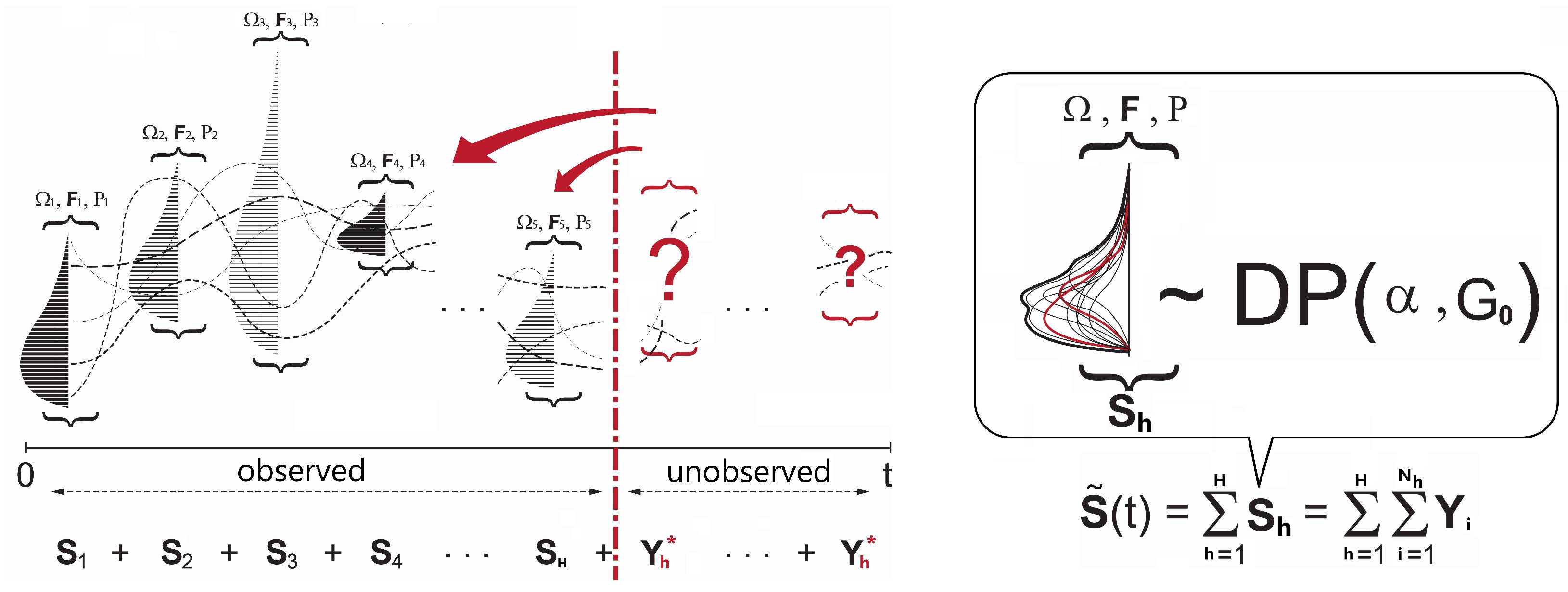
Figure 2. An example of looping through the Gibbs sampler with complete data. In Step I, the algorithm requires the initial cluster memberships and parameters. In Step II.(A), based on the Chinese Restaurant scheme [19] with the DPM prior (

G_{0}

), the probabilities of the selected observation h being in each current and the proposed new cluster are computed, which updates the cluster memberships. In Step II.(B), the new continuous cluster membership is determined by a multinomial distribution with a set of the resulting cluster probabilities from Step II.(A) randomly assigned based on the Polya Urn scheme. Once all observations have been assigned to clusters at a given iteration in the Gibbs sampler, then the parameters are updated, given cluster membership.

G_{0}

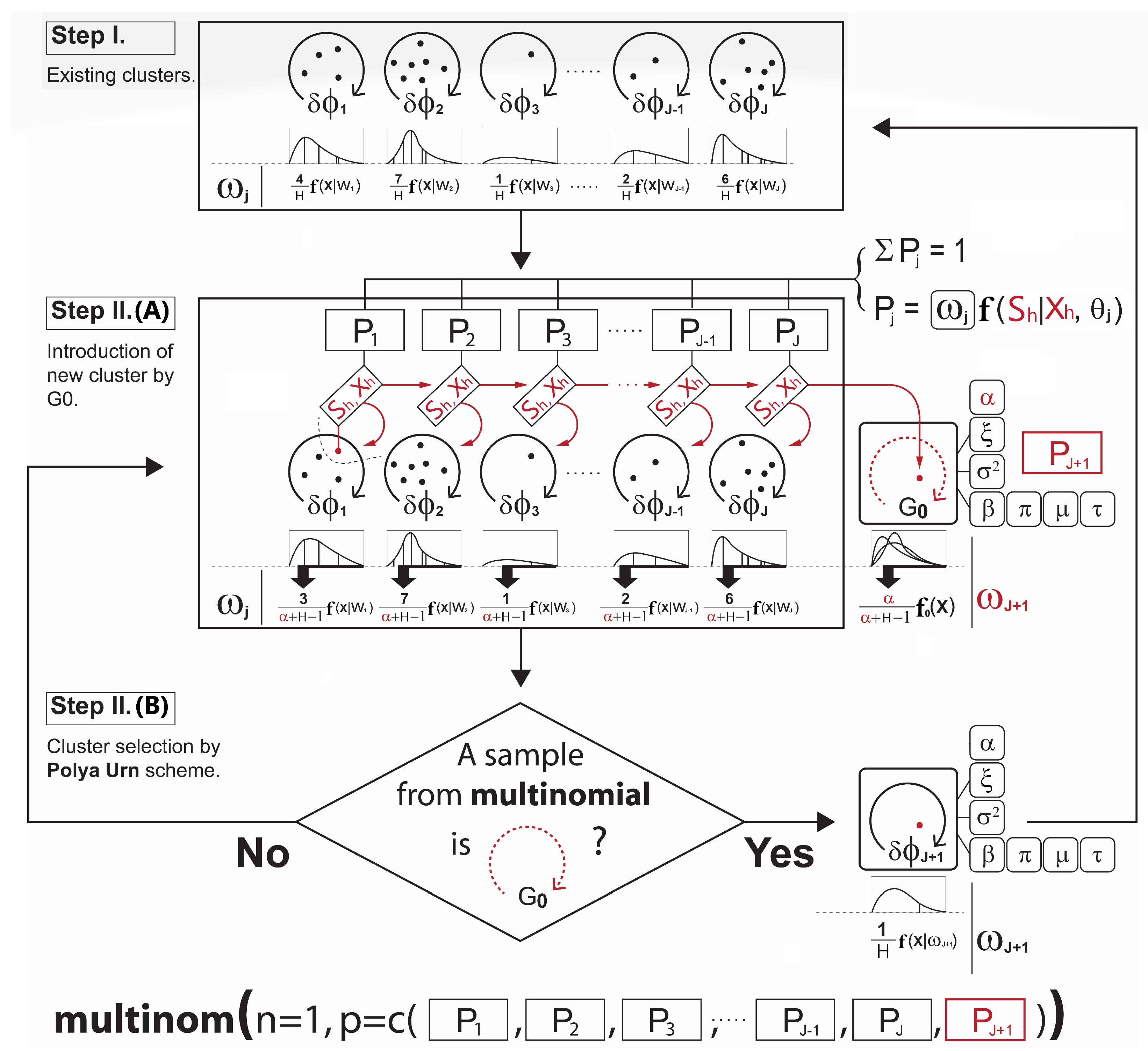
Figure 3. An example of a re-clustering process with MAR imputation in the DPM Gibbs sampler: Step I and II. The imputations are made cluster membership-wise. Each imputation model as a joint distribution is the product of the outcome model and the covariate model that has missing data.

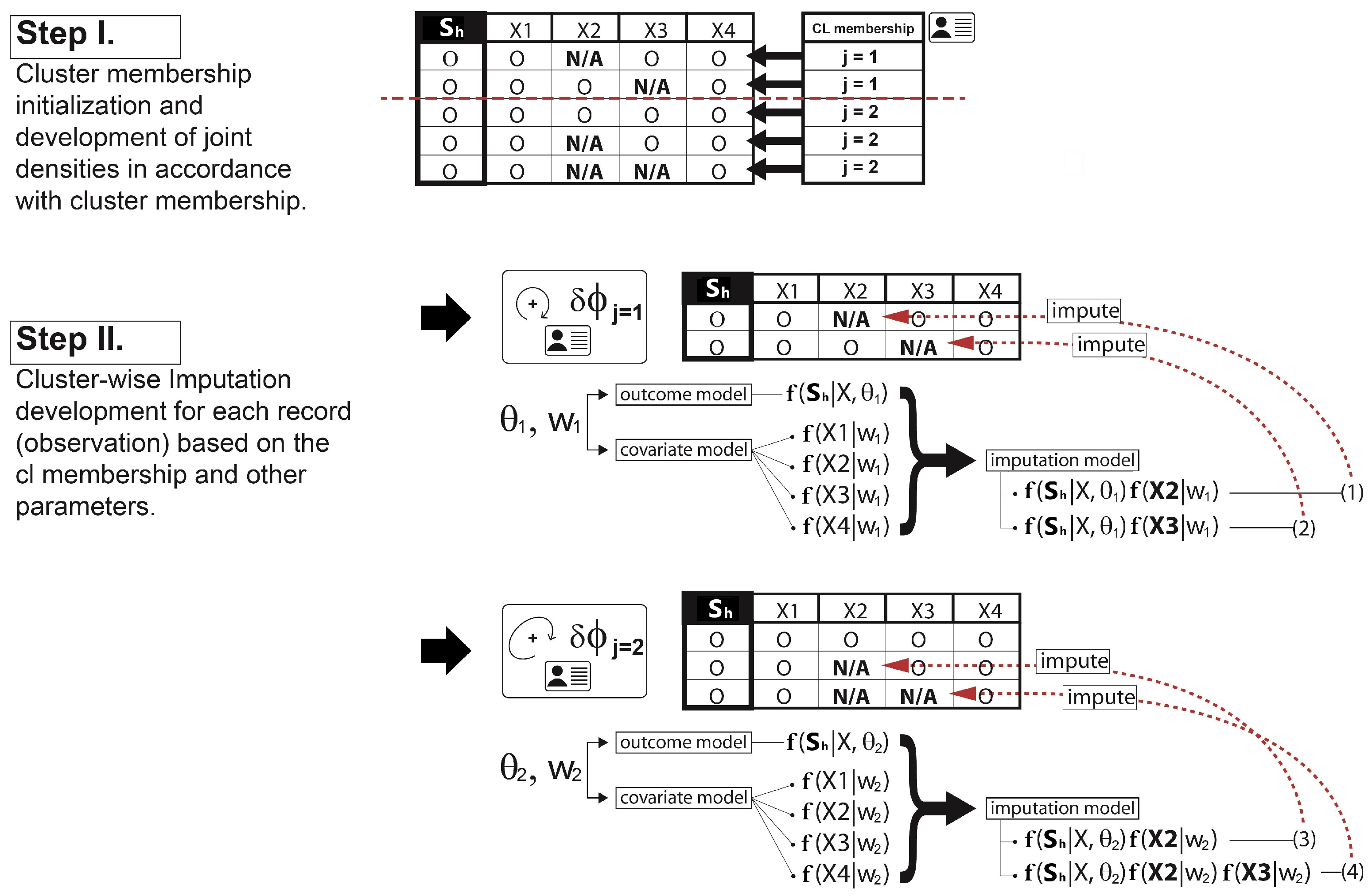
Figure 4. An example of a re-clustering process with MAR imputation in the DPM Gibbs sampler: Step III. The DPM refines the outcome models for all possible configurations based on the types of missingness prior to running the Gibbs sampler. Using these outcome models, each cluster probability and the predictive density are updated.

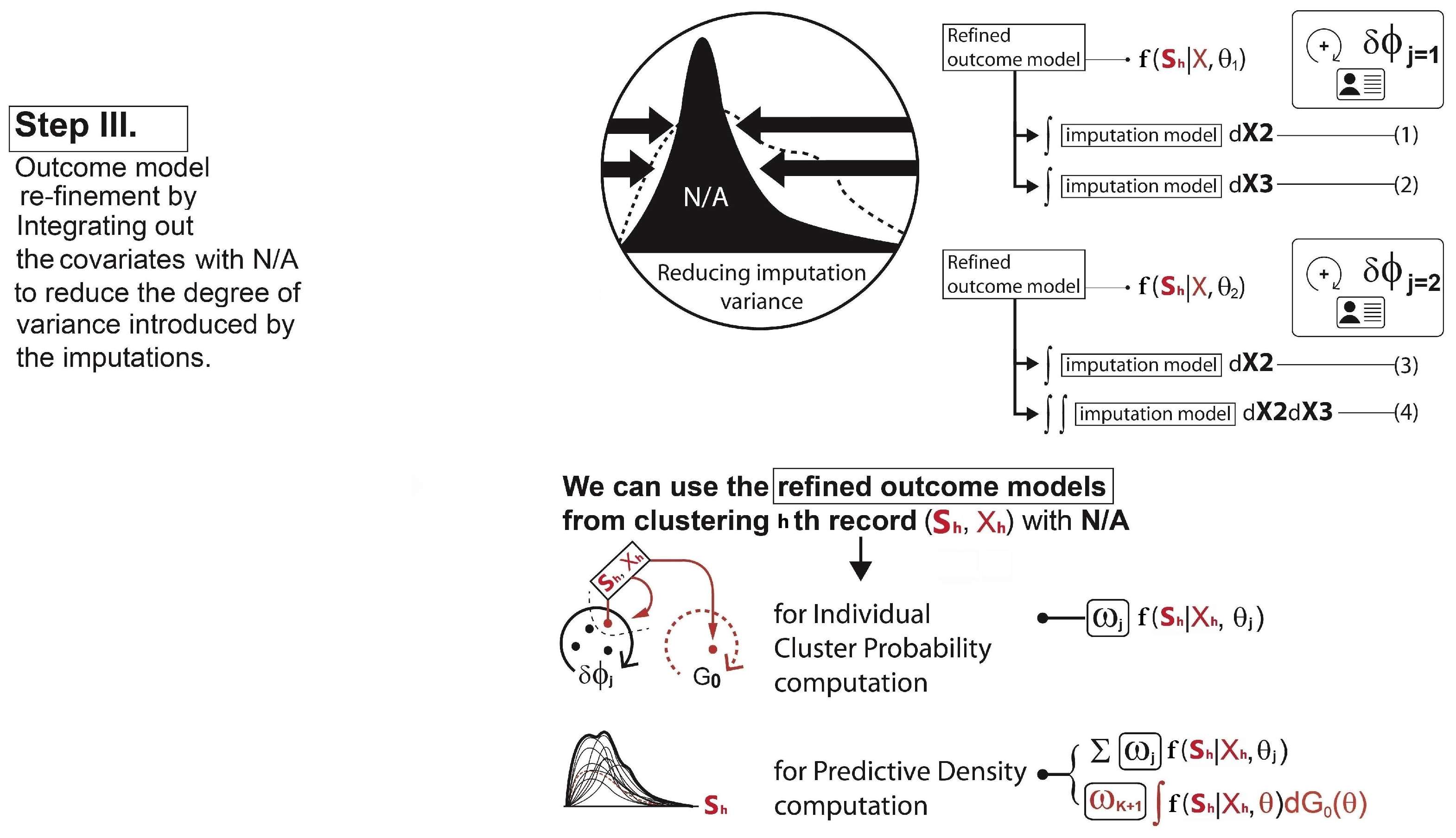
Figure 5. Parameter re-estimation after the re-clustering with imputation in the Gibbs sampler. This diagram articulates flows of the parameter updates, using the acyclic graphical representation. The process cycles until achieving convergence.

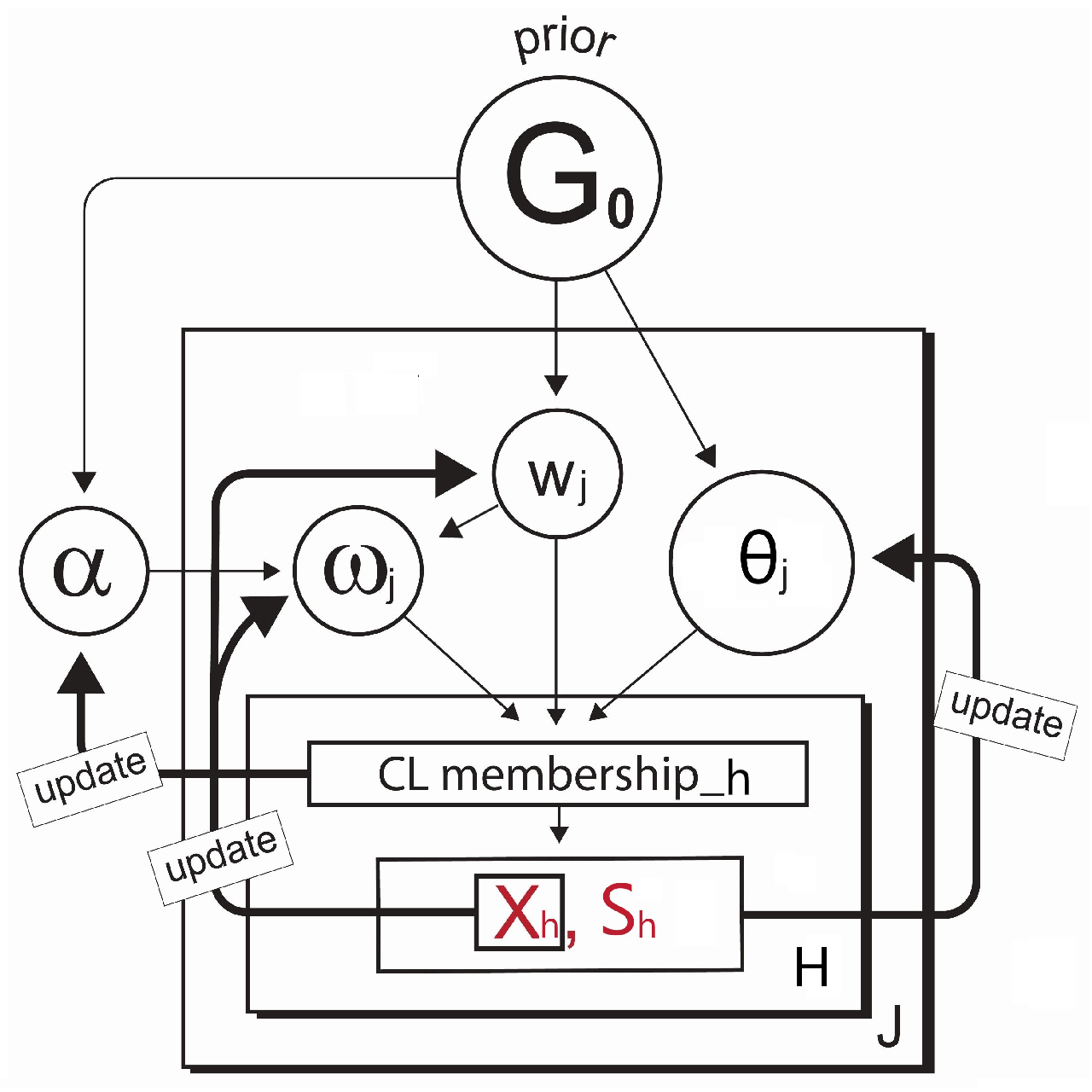
Figure 6. Histograms of the outcomes and log-transformed outcomes for the two datasets: (a) PnCdemand, (b) LGPIF.

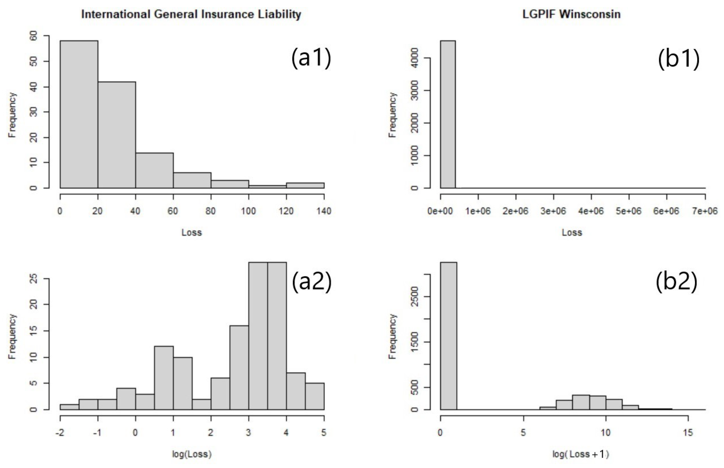
Figure 7. LogN-DPM: The last 100 in-sample predictive densities (scenarios) overlaid together.

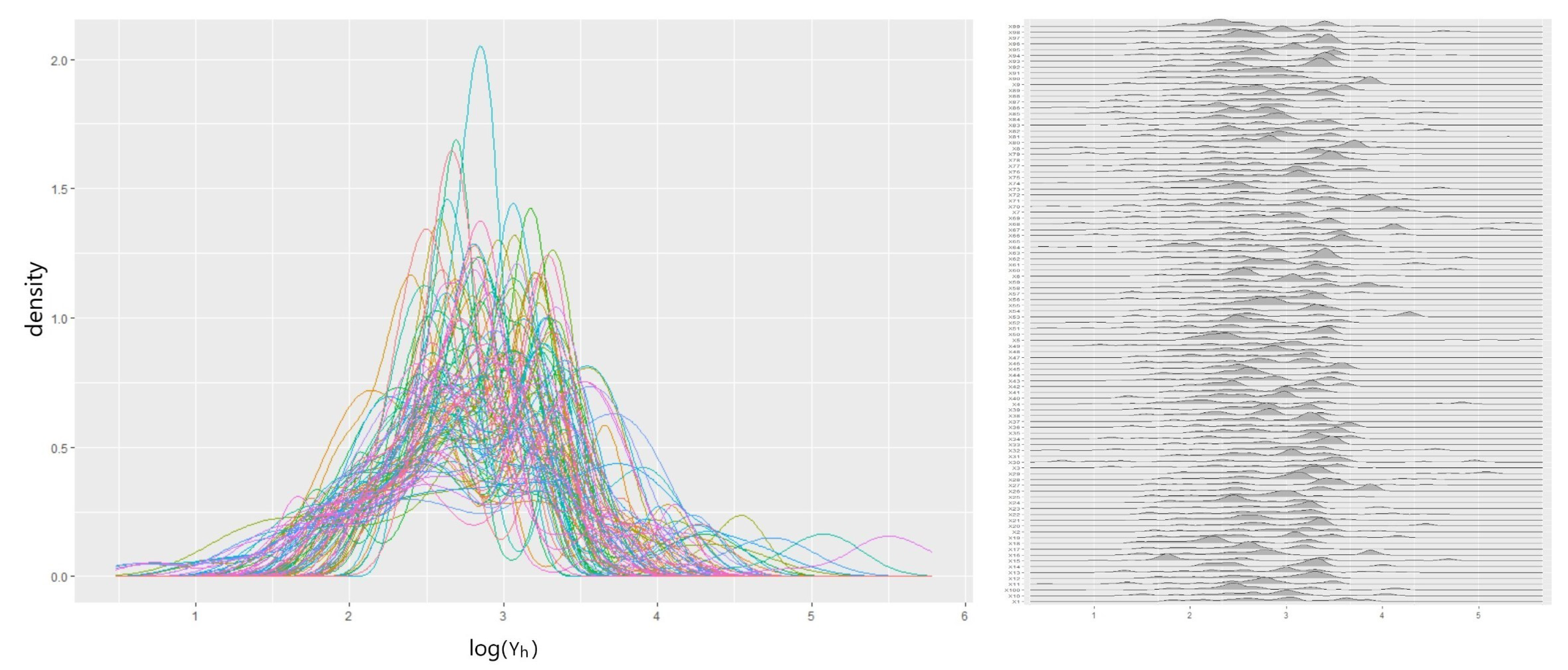
Figure 8. MICE trace plots and in-sample predictive densities produced from GLM, GAM, MARS.

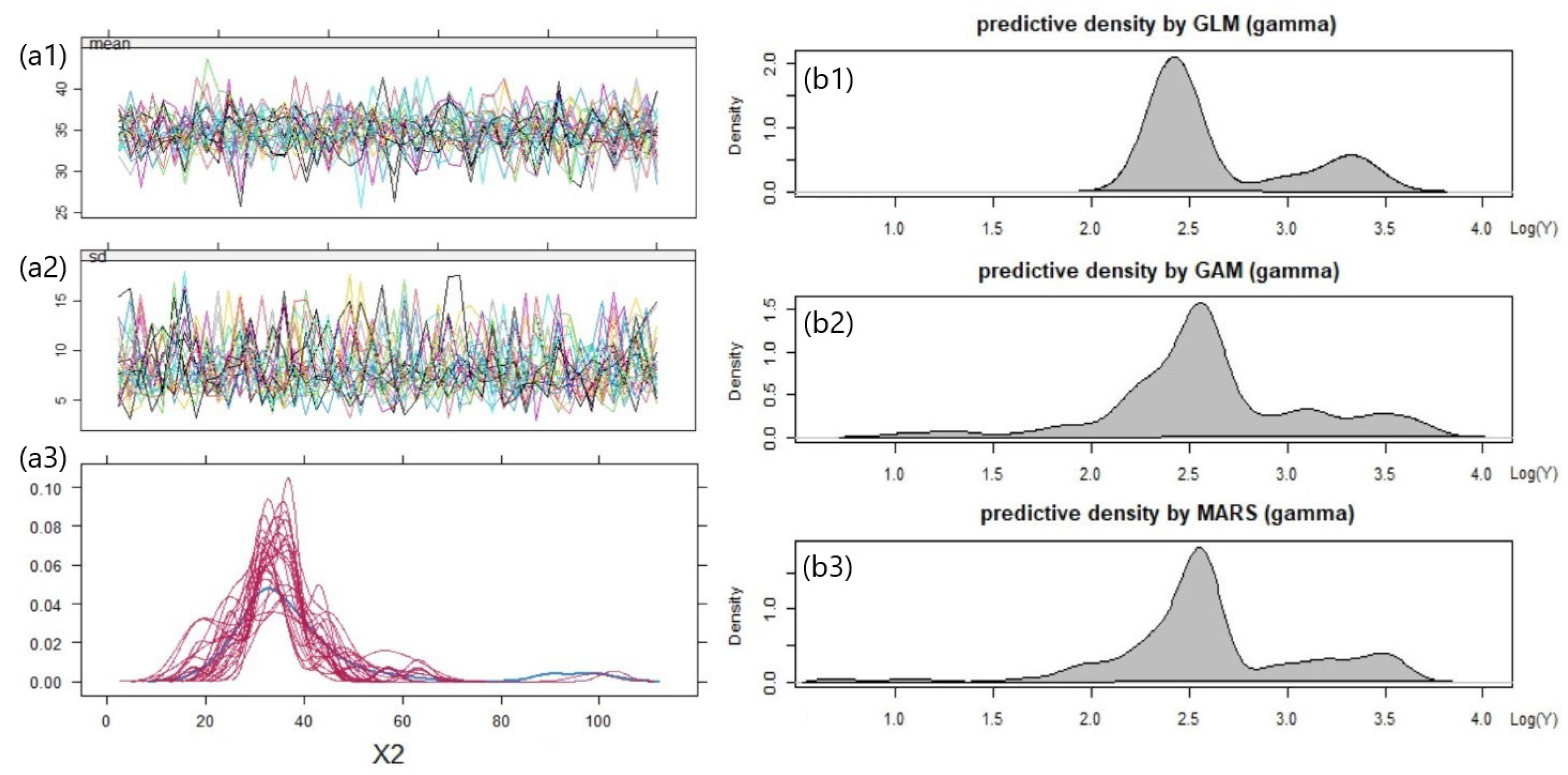
Figure 9. A histogram of the observed loss

Y_{h}

on the log scale and the out-of-sample predictive densities for the typical class of a policy.

Figure 9. A histogram of the observed loss

Y_{h}

on the log scale and the out-of-sample predictive densities for the typical class of a policy.

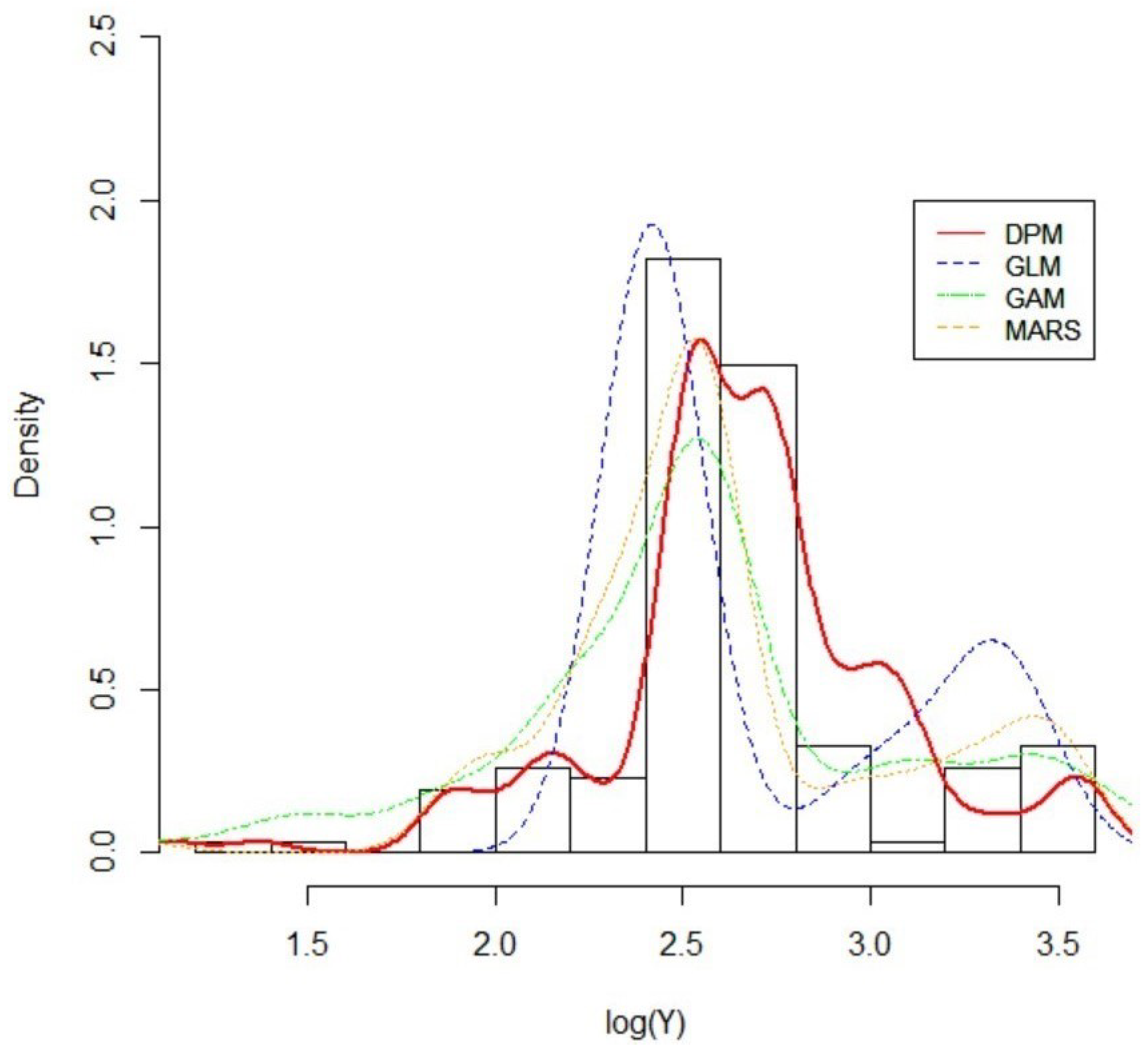
Figure 10. LogSN-DPM: The last 100 in-sample predictive densities (scenarios) overlaid together.

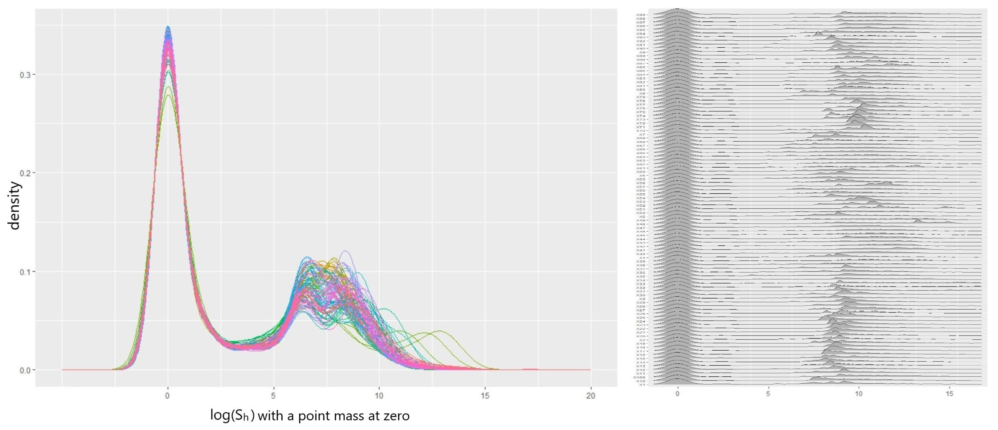
Figure 11. MICE trace plots and in-sample predictive densities produced from GLM, GAM, MARS.

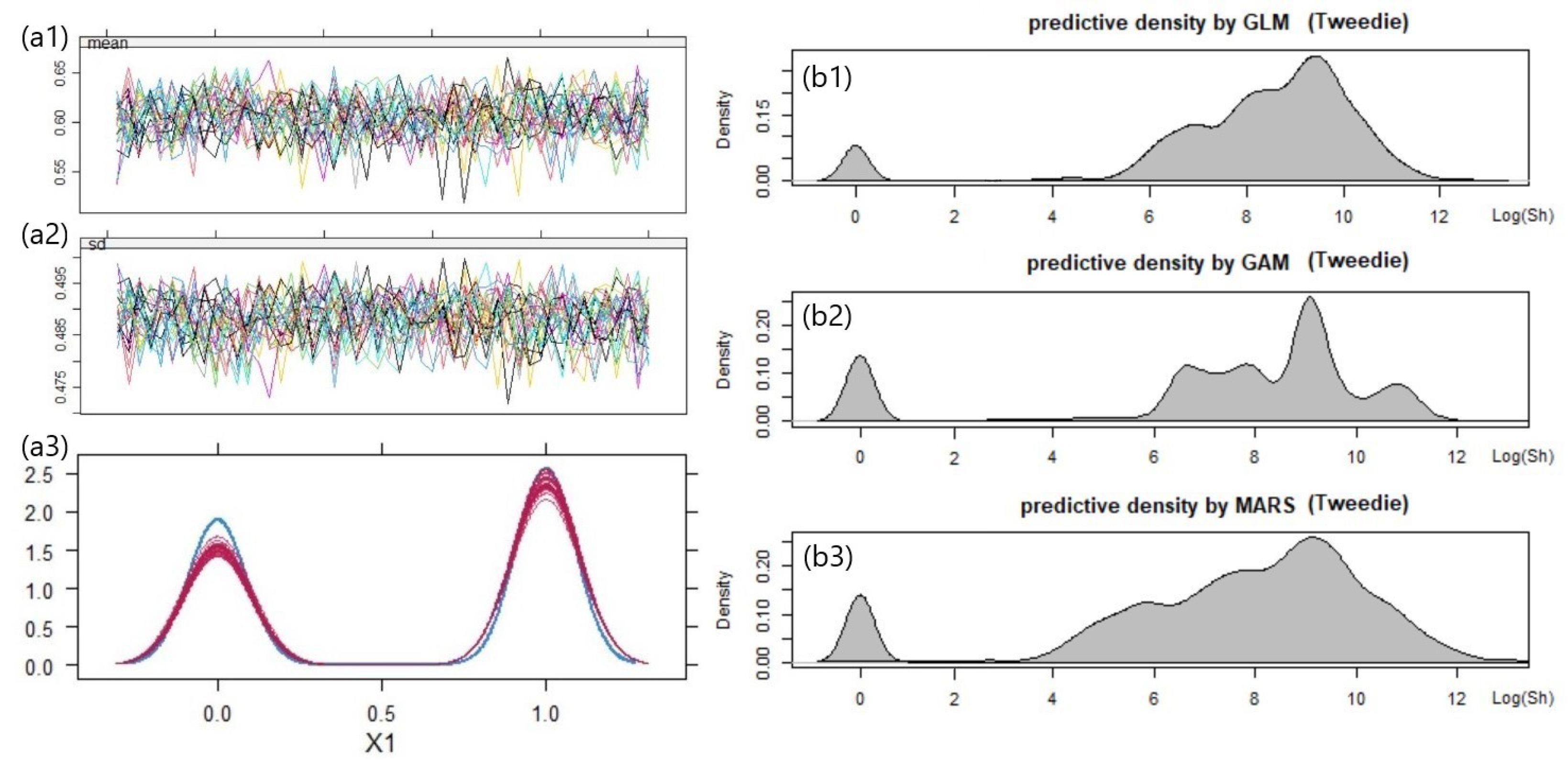
Figure 12. A histogram of the observed total loss

S_{h}

on the log scale and the out-of-sample predictive densities for the typical class of a policy.

Figure 12. A histogram of the observed total loss

S_{h}

on the log scale and the out-of-sample predictive densities for the typical class of a policy.

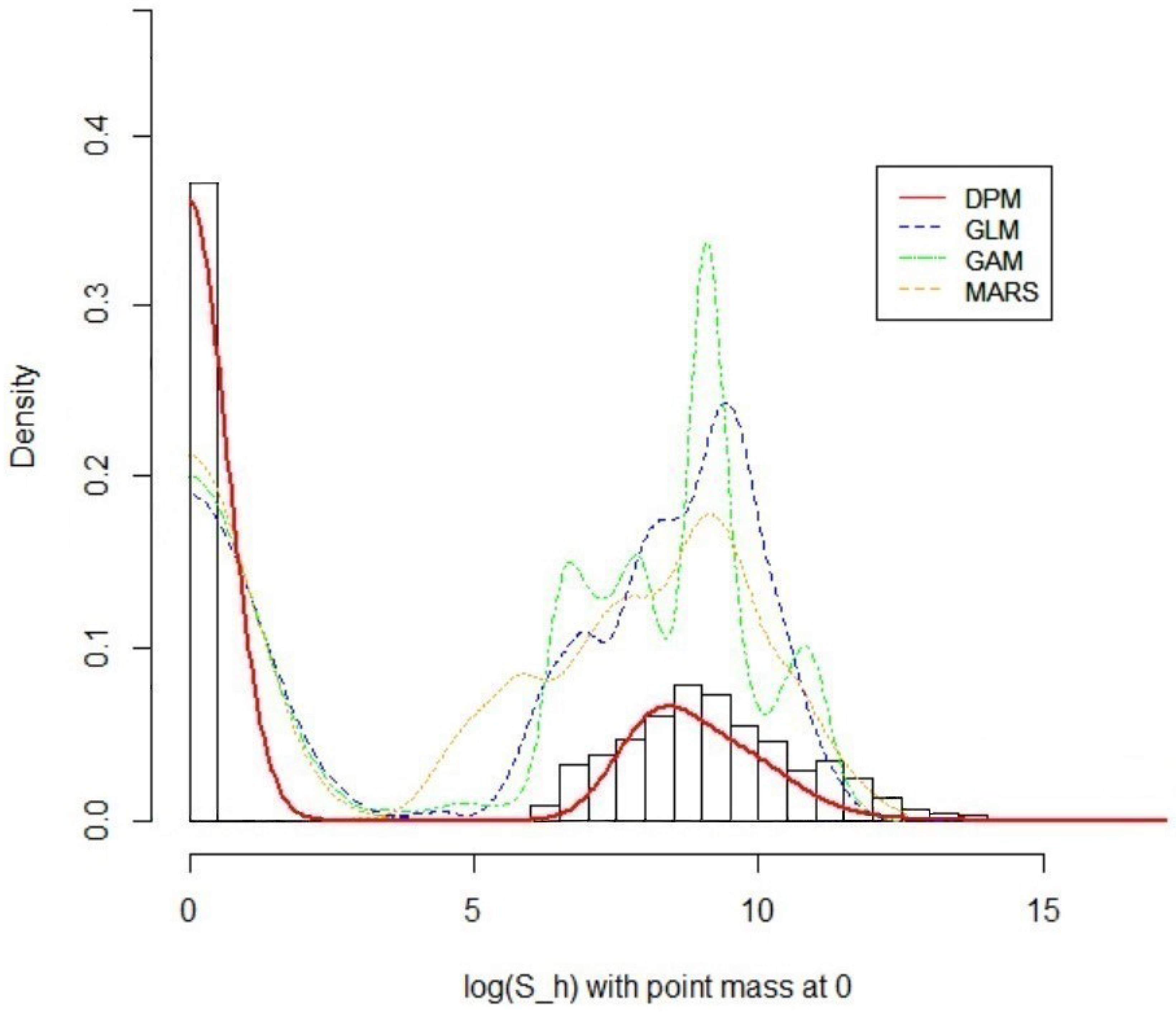
Table 1. The comparison of out-of-sample modeling results based on the dataset PnCdemand.

Model	AIC	SSPE	SAPE	10% CTE	50% CTE	90% CTE	95% CTE
Ga-GLM	830.56	268.6	139.8	6.5	13.8	54.5	78.0
Ga-MARS	830.58	267.2	138.2	6.1	13.0	57.2	71.1
Ga-GAM	845.94	266.7	136.1	6.2	13.3	58.1	72.2
LogN-DPM	-	272.0	134.7	6.4	13.8	59.3	79.3

Table 2. The comparison of out-of-sample modeling results based on the LGPIF dataset

Model	AIC	SSPE	SAPE	10% CTE	50% CTE	90% CTE	95% CTE
Tweedie-GLM	26270.3	2.04e+14	89380707	955.9	12977.2	133374.4	340713.1
Tweedie-MARS	24721.4	1.99e+14	88594850	961.7	10391.0	129409.2	355112.6
Tweedie-GAM	21948.9	1.95e+14	88213987	989.4	13026.2	140199.5	398263.1
LogSN-DPM	-	1.98e+14	83864890	975.3	13695.1	147486.6	425682.6

Disclaimer/Publisher’s Note: The statements, opinions and data contained in all publications are solely those of the individual author(s) and contributor(s) and not of MDPI and/or the editor(s). MDPI and/or the editor(s) disclaim responsibility for any injury to people or property resulting from any ideas, methods, instructions or products referred to in the content.

© 2023 by the authors. Licensee MDPI, Basel, Switzerland. This article is an open access article distributed under the terms and conditions of the Creative Commons Attribution (CC BY) license (http://creativecommons.org/licenses/by/4.0/).

Copyright: This open access article is published under a Creative Commons CC BY 4.0 license, which permit the free download, distribution, and reuse, provided that the author and preprint are cited in any reuse.

Downloads

116

Views

Comments

Subscription

Notify me about updates to this article or when a peer-reviewed version is published.

MDPI Initiatives

Important Links

Choose an area of interest and we will send you notifications of new preprints at your preferred frequency.

Disclaimer

Dirichlet Process Log Skew-normal Mixture with Missing at Random Covariate in Insurance Claim Analysis

Abstract

Keywords:

Subject:

1. Introduction

2. Discussion on Research Questions and Related Work

2.1. Can Dirichlet Process Capture the Heterogeneity and Bias?: RQ1, RQ2

2.2. Can Log Skew-Normal Mixture Approximate the Log-Normal Convolution?: RQ3

2.3. Our Contribution and Paper Outline

3. Model: DP Log Skew-Normal Mixture for S h | X

3.1. Background

3.2. Model Formulation with Discrete and Continuous Clusters

3.3. Modelling S h | X h with Complete Case Covariate

3.4. Modelling S h | X h with MAR Covariate

4. Bayesian Inference for S h | X h with MAR Covariate

4.1. Parameter Models and MAR Covariate

4.2. Data Models and MAR Covariate

4.3. Gibbs Sampler Modification for MAR Covariate

5. Empirical Study

5.1. Data

5.2. Three Competitor Models and Evaluation

5.3. Result 01. International General Insurance Liability Data

5.4. Result 02. LGPIF Data

6. Discussion

6.1. Research Questions

6.2. Future Work

7. Variable Definitions

Author Contributions

Data Availability Statement

Acknowledgments

Conflicts of Interest

Appendix A Parameter Knowledge

Appendix A.1. Prior Kernel for Distributions of Outcome, Covariates, and Precision

Appendix A.2. Posterior Inference for Outcome, Covariates, and Precision

Appendix B Baseline Inference Algorithm for DPM

Appendix C Development of the Distributional Components for DPM

Appendix C.1. Derivation of the Distribution of Precision α

Appendix C.2. Outcome Data Model of S h Development with MAR Covariate x 1 for the Discrete Clusters

Appendix C.3. Covariate Data Model of x 2 Development with MAR Covariate x 1 for the Continuous Clusters

References

MDPI Initiatives

Important Links

Subscribe

3. Model: DP Log Skew-Normal Mixture for $S_{h} | X$

3.3. Modelling $S_{h} | X_{h}$ with Complete Case Covariate

3.4. Modelling $S_{h} | X_{h}$ with MAR Covariate

4. Bayesian Inference for $S_{h} | X_{h}$ with MAR Covariate