An Intelligent Bat Algorithm for Web Service Selection with QoS Uncertainty

Preprint

Article

An Intelligent Bat Algorithm for Web Service Selection with QoS Uncertainty

Altmetrics

Downloads

103

Views

Comments

A peer-reviewed article of this preprint also exists.

Abdelhak ETCHIALI^*,

Amina BEKKOUCHE,Fethallah HADJILA

Abdelhak ETCHIALI^*,

Amina BEKKOUCHE,Fethallah HADJILA

This version is not peer-reviewed

Submitted:

27 May 2023

Posted:

02 June 2023

You are already at the latest version

Alerts

Abstract

Nowadays, the selection of web services with uncertain quality of service (QoS) is gaining a lot of attention in the service-oriented computing paradigm (soc). In fact, searching for a service composition that fulfills a complex user’s request is known to be NP-Complete. The search time is mainly dependent on the number of the requested tasks, the size the available services, and the size of the QoS realizations (i.e., sample size). To handle this problem, we propose a two-stage approach that reduces the search space using heuristics for ranking the tasks’ services and a bat algorithm metaheuristic for selecting the final near optimal compositions. The fitness used by the metaheuristic aims to fulfill all the global constraints of the user. The experimental study shows that the ranking heuristics, termed “fuzzy pareto dominance” and "Zero-order stochastic dominance", are highly effective than the other heuristics and most of the existing state-of-the-art methods.

Keywords:

Subject: Computer Science and Mathematics - Artificial Intelligence and Machine Learning

1. Introduction

With the advent of cloud computing and specifically the online services (SaaS), it becomes more challenging to discover and select the best services with respect to user’s requirements [1,2]. Broadly speaking, we observe that a given functionality can be fulfilled by numerous SaaS services with a variety of QoS levels. For complex user’s requests (in terms of workflow) the task of selecting the best composition of services that satisfies the user’s global constraints (e.g., the maximum cost of the composition of services is less than a given budget) is time consuming and far from meeting the user’s expectations. It is worth noting that the selection of service compositions is NP-complete and exponentially depends on the number of tasks of the workflow (see the example of Table I). In practice, we observe that the QoS of SaaS applications is inherently uncertain and always changing; for instance, the cost of booking a hotel chamber or an airline ticket is uncertain and depends on the period (such as the season or month), social events, and other contextual Aspects. To compare the services of the same functionality class while considering the different realizations of the QoS criteria, one can use statistical measures such as the mean QoS value or the median value to derive the best alternatives. Unfortunately, these measures may not be effective as it will be explained using the example of Table 1.

In the same line of thought, we point out that the pertinence of service compositions with respect to the user’s request is no longer a deterministic score, but it is rather specified as a probability of satisfying the global QoS constraints; this score is termed Global QoS Conformance (GQC) [3]. As a result, the complexity of the selection issue is dependent on the number of tasks and also is impacted by both the size of each task and the size of the QoS sample (i.e., the number of realizations per QoS attribute).

GQC can be also seen as the expected value of the a random variable termed Z, where Z provides an outcome equal to 1 if the aggregated QoS satisfy the global constraint bound; moreover, it is highly desirable to get service compositions that satisfy a maximum number of global constraints in terms of median QoS (this means that 50% of the solution realizations -of a single QoS attribute- will ensure the end-to-end bounds). This criterion is denoted as the percentage of satisfied global constraints (PSGC). This latter measure can be considered (sometimes) as an alternative to the GQC objective function, since it ensures a high gain of computational cost. For instance, according to Table I, where the global constraint (GC) is specified in the first line, we observe that only (s1,s10) and (S2,s10) will be retained as feasible solutions since PSGC=100% (the example is comprised of a single QoS attribute); however, the remaining compositions are not feasible, and therefore PSGC=0.

To summarize, our selection issue needs effective ranking heuristics for the workflow tasks, as well as time-efficient approaches for exploring the service compositions. To address these difficulties, we propose a two-stage approach that ensures high fitness service compositions and acceptable responsiveness delay.

In the first step, we reduce the search space in each task by only retaining the TopK pertinent services in terms of a given heuristic

H_{i}

. Consequently, the total search space is reduced from

m^{n}

candidate solutions to

k^{n}

candidate solutions, where n stands for the number of tasks and m stands for the number of services per task (see Table 2 for more details).

In the second step, we perform a heuristic global search (this means that our solution will be a vector of n services) and retain the TopK compositions in terms of GQC.

Our contributions can be summarized as follows:

We downsize our search space from $m^{n}$ to $k^{n}$ by retaining the most pertinent elements of each task. To this end, we propose four ranking heuristics of the items of each task. All these heuristics perform pairwise comparisons of services and select TopK elements having the maximum number of wins.

-

$H_{1}$ is an efficient implementation of the fuzzy pareto dominance; it is inspired from [33].

-

$H_{2}$ (zero order stochastic dominance) is a stochastic dominance relationship that uses the zero order terms of the QoS sample [34]. it directly uses the QoS realizations during the comparisons.

-

$H_{3}$ (first order stochastic dominance) is a stochastic dominance relationship that uses the first order terms of the QoS sample [34]; this means that $H_{3}$ uses the cumulative distribution of the sample to perform comparisons.

-

$H_{4}$ (the majority interval heuristic) is inspired from [19]. In this ranking, we compute the median interval of each service and perform pairwise comparisons of services using equation 27. the services having the highest number of wins are retained in TopK elements.
In the second step, we perform a global search on the retained TopK services using a swarm intelligence-based algorithm termed "discrete bat algorithm (DBA)". This metaheuristic is chosen because of its ability to leverage both global search operators and local search operators during the exploration of candidate solutions (in contrast to metaheuristics that only use one operator such as particle swarm optimization or ant colony optimization). The coordinated use of these operators can achieve promising results on NP-complete problems.
At the end, We evaluate the effectiveness and the efficiency the approach using a consolidated set of experiments.

The rest of this paper is organized as follows: Section 2 presents a literature overview of the existing works. Section 3 specifies the problem statement. In Section 4, we introduce the proposed approach as well as the selection algorithms. In section5, we present a set of experimental evaluations and compare our method with existing works. Section 6 concludes the paper and presents future perspectives.

2. State of the Art

Selecting service compositions using QoS is a major topic in service-oriented computing (SOC), We mainly distinguish two categories: service selection with certain (deterministic) QoS and service selection with uncertain (nondeterministic) QoS, we will review the to parts in what follows.

2.1. Service Selection with Certain QoS

In this category, we assume that the QoS attributes are static and do not change overtime, therefore the evaluation function of compositions is also deterministic. Many works and reviews have been proposed to address this kind of issues ([1,4,5,6]). In what follows, we will discuss the most important ones.

[7] proposed a framework that first takes the skyline services of each task; then, a set of service clusters (within each task) are hierarchically created using K-means to lower the size of the search space. At the end, the solutions are explored using the combinations of cluster-heads. The work by [8] decomposes global QoS constraints into local constraints using culture genetic algorithm, then the top items are selected to aggregate the final compositions.

[4] adopted both functional ( the function signature) and nonfunctional attributes (QoS, global constraints) to select the Top-K service compositions. The authors leveraged harmony search to derive the compositions that best meet the complex requirements.

[9] used the multi-criteria decision method termed Topsis to search the most promising services in terms of QoS. The proposal leveraged six QoS criteria with different workflow patterns and constructs.

[10] leveraged both local and global search for tackling the selection of cloud services. The local selection allows for downsizing the search space, while the global selection allows for keeping near-optimal compositions.

[11] tackled the optimal selection of web services by adopting both PetriNet models and skyline search; these authors also used the R- tree structure to accelerate the search for Pareto-optimal solutions.

In [5], the authors used an optimized artificial bee colony (oabc) method for service composition. Mainly, the authors introduced three ideas in the initial bee algorithm: the first one is the diversification of the initial population; the second one is the dynamic adjustment of the neighborhood size of the local search; the third one is the addition of a global movement operator that aims to get closer to the global solution. The work by [12] leverages fuzzy dominated scores to derive the TopK services that have more balanced QoS (and which can be better than some skyline services with undesirable QoS values) in a self-contained task. [13] considered self-organising migrating algorithm (SOMA) and fuzzy dominance relationship to aggregate service workflows. The fuzzy dominance function is used in the SOMA meta heuristic to compute the QoS aware distances between services. [14] proposed a bio-inspired method termed enhanced flying ant colony optimisation (EFACO). This approach constrains the flying activity and handles the execution time problem by a modified local selection. Since this phase may degrade the selection quality, a multi-pheromone approach is adopted to enhance the exploration through the pheromone assignment to each QoS criterion.

[15] clustered the cloud services using a trust-oriented k-means, then they created the composition of cloud services using honey bee mating. It is worth noting that the proposed framework is not scalable for large datasets. The work by [16] tackled the service selection problem by handling multiple users’ requirements. The approach is comprised of two steps: firstly, an approximate pareto-optimal set is computed using approximate dominance; secondly, the near optimal compositions are selected using artificial bee colony algorithm.

2.2. Service Selection with Uncertain QoS

The work of [17] is one of the earliest works that addresses the service selection with uncertain QoS. The authors proposed a excellent heuristic termed, P-dominant skyline, to derive the best QoS aware services in a self-contained task. P-dominant skyline is considered to be resilient to QoS inconsistencies and noise. Moreover, this heuristic is accelerated using R-trees. [18] adopted probability distributions to model the QoS uncertainty of service workflows. To select the best compositions, the authors used both integer programming and global constraints penalty cost functions.

[19] proposed a promising heuristic to derive the pertinent services of local tasks using majority intervals. The main idea consists of computing the median interval of each nondeterministic QoS attribute and comparing them using rectified linear unit functions (RelU) [20]. After that, an exhaustive search is applied to get the final compositions. In [21], the authors proposed a set of heuristics for ranking the services of the workflow tasks. These propositions include probabilistic dominance relationships and fuzzy dominance alternatives. Once the TopK elements are retained from each task, a constraint programming approach is applied to retain the TopK optimal compositions of services. [22] addressed the service composition issue by handling the QoS uncertainty and the location awareness. They proposed a sophisticated approach that combines the firefly metaheuristic with a fuzzy logic-based web service aggregation.

The framework proposed in [23] sorted the services of each task using both entropy and variance of the QoS attributes, the services that have larger values in terms of entropy and variance are discarded since they are considered as noisy or inconsistent services. Then, the items having the lowest entropy/variance scores were retained to compose the final solutions.

[3] is one of the first works that handled of QoS uncertainty and composition. Based on ideas defined in [24], the strategy adopted by the authors consists of decomposing the end-to-end constraints into local constraints; the local edges (entrances) are calculated by dividing the end-to-end constraint bounds in proportion to the aggregated median QoS of each class of the workflow. After that, an initial service composition is built using a predefined utility function. If this latter one is not optimal, the method searches for alternative solutions using simulated annealing. In the same line of thought, [25] introduced a proposition for Web service selection with presence of outliers. Contrary to the work of [3], this method leverages a different heuristic to divide the end-to-end constraints into local constraints. The proposed idea ensures a high resilience with respect to outliers (services with noisy or unusual QoS). The work by [26] leverages stochastic dominance relationship to sort the services of each task of the user’s workflow; after that, a backtracking search is applied to the filtered tasks to derive optimal service compositions. [27] proposed an interval-based multi-objective bee colony method to address the uncertain QoS-aware service composition problem. The authors proposed an interval-oriented dominance relationship for comparing the services using intervals that represent the variation range of QoS attributes. In addition an interval-valued utility function is introduced to assess the quality of a composition with QoS uncertainty. Finally, an improved version of NSGA-II is used to derive the non-dominated service compositions. The framework proposed in [28] involves two steps: the first one retains the pertinent services of the local tasks using majority grades, and the second step performs a constraint programming search to keep the optimal compositions. In the same line of thought, the work by [29], proposes a heuristic for filtering the desirable services of each local task using hesitant fuzzy sets and cross entropy, then a metaheuristic termed grey wolves optimization is applied to retain the TopK near optimal service compositions.

3. Problem Specification

In what follows, we introduce the formalism used in handling the selection of service compositions with QoS uncertainty.

3.1. Parameters’ Notation

To tackle our problem, we use the notation shown in Table 2. We assume that the user’s workflow is composed of n sequential tasks cl₁, cl₂,...,cl_n, each task is achieved by a service s_i that has r QoS attributes. Each QoS criterion is materialized by a sample of l realizations (see Table 2 and Figure 1).

3.2. QoS model

In this work, we will only consider positive QoS attributes (i.e., those that need to be maximized). For negative attributes, we will simply multiply them by -1 and treat the new versions as positive ones. We note that our workflow is composed of n sequential tasks. The aggregated QoS of a workflow (having different patterns such as sequence, loops, parallelism, and choice) is presented in [7,30].

3.3. Global QoS Conformance

The measure of Global QoS Conformance (GQC) [3] is leveraged to rank the TOPK compositions. GQC is the probability that the composition of services satisfy all global constraints (see Equation 1). In particular, we say that a composition C is better than another composition

C^{'}

if the GQC of C is higher than that of

C^{'}

with respect to Equation 1. If C ties with

C^{'}

, then we sort them according to the utility (

U (.)

) function that is shown in Equation 4, the larger the score of

U (.)

, the better the rank.

Our aim is to search the compositions

C (s_{w 1}, \dots, s_{w n})

such that GQC is maximized:

G Q C ((S_{w_{1}}, \dots, S_{w_{n}}), (b_{1}, \dots, b_{r})) =

\prod_{p = 1}^{r} C C ((S_{w_{1}}, \dots, S_{w_{n}}), b_{p})

(1)

Since we assume that the QoS criteria are independent, the global QoS conformance is defined as the product of constraint conformances (CC for short).

The criterion CC is defined as:

C C ((S_{w_{1}}, \dots, S_{w_{n}}), b_{p}) =

\frac{1}{l^{n}} \sum_{u_{1} = 1}^{l} \dots \sum_{u_{n} = 1}^{l} s t e p (a g g r e g a t e (Q o S_{p w_{1} u_{1}}, \dots, Q o S_{p w_{n} u_{n}}), b_{p})

(2)

The function CC computes the satisfaction degree of a single global constraint. Finally, the binary function “Step” is defined as:

S t e p (A g g r e g a t e (Q o S_{p w_{1} u_{1}}, \dots, Q o S_{p w_{n} u_{n}}), b_{p}) =

\{\begin{matrix} 1 & if A g g r e g a t e (s_{p w_{1} u_{1}}, \dots, Q o S_{p w_{n} u_{n}}) \geq b_{p} \\ 0 & otherwise \end{matrix}

(3)

\begin{matrix} U (C) = \sum_{p = 1}^{r} w_{p} * \frac{(M e d i a n Q_{p}^{'} (C) - Q {m i n}^{'} (p))}{(Q {m a x}^{'} (p) - Q {m i n}^{'} (p))} \end{matrix}

(4)

Q {m i n}^{'} (p) = \sum_{j = 1}^{n} Q m i n (j, p)

(5)

Q {m i n}^{'} (p)

is the minimal aggregated QoS of the p^th attribute for all possible compositions.

Q {m a x}^{'} (p) = \sum_{j = 1}^{n} Q m a x (j, p)

(6)

Q {m a x}^{'} (p)

is the maximal aggregated QoS of the p^th attribute for all possible compositions.

The Equations

Q m i n (j, p), Q m a x (j, p)

are defined as follows :

Q m i n (j, p) = M i n_{u \in {1, \dots, l}, s_{i} \in c l_{j}} (Q o S_{p i j u})

(7)

Q m i n (j, p)

is the minimal QoS value of the p^th attribute of all services related to the i^th task.

Q m a x (j, p) = M a x_{u \in {1, \dots, l}, s_{i} \in c l_{j}} (Q o S_{p i j u})

(8)

Q m a x (j, p)

is the maximal QoS value of the p^th attribute of all services related to the i^th task.

M e d i a n {Q p}^{'} (C) = \sum_{j = 1}^{n} M e d i a n_{u \in {1, . . ., l}} Q o S_{p s_{j} j u}

(9)

By assuming that the criterion p is positive, the global constraint with respect to the median value is specified as:

M e d i a n {Q^{'}}_{p} (C) \geq b_{p}; \forall p \in {1, . . ., l}

(10)

By assuming that the p ^th attribute is aggregated with a sum function,

M e d i a n Q_{p}^{'} (C)

represents the aggregated QoS of C with respect to the median QoS value of each component of C (of the p^th attribute).

Equation 10 is used to determine whether the global constraints are respected or not by the composition C.

To clarify the computation of the previous equations, we continue with the example cited in Table I:

${M e d i a n Q}^{'}_{p} (C = < s_{1}, s_{10} >) = 20 + 26 = 46 \geq 45$ .
$G Q C (C) = 16 / 25 = 0.64$

If $Q m i n (1, 1) = Q m i n (2, 1) = 0$ and $Q m a x (1, 1) = Q m a x (2, 1) = 300$ , then
$U (C) = \frac{46 - 0}{(600 - 0)} = 0.075$

The composition C is feasible.

However, if the components of $C^{'}$ are $< s_{3}, s_{13} >$ then:
${M e d i a n Q}^{'}_{p} (C^{'} = < s 3, s_{13} >) = 18 + 10 = 28 \leq 45$ .
$G Q C (C^{'}) = 9 / 25 = 0.36$
$U (C^{'}) = \frac{28 - 0}{(600 - 0)} = 0.046$ .

The composition $C^{'}$ is not feasible because it violates the global constraint.

4. Proposed Approach

In what follows, we present the architecture of the proposed solution as well as the different implemented algorithms. (see Figure 2).

4.1. Overall Architecture

Our proposed framework involves three principal parts:

The workflow building and update module: Its goal is to assign the new services to their corresponding tasks (a task is a functionality available on the internet, e.g., hotel booking). This component also updates the tasks by changing/removing the services.
The QoS update and management module: It stores all the QoS realizations of all services in a data-warehouse; The QoS information may stem from different sources such as social networks (e.g., ratings, fidelity), third parties (e.g., throughput, latency), and service providers (e.g., cost).
The QoS aware service selection engine: Given a user’s workflow and the set of global constraints, the selection module allows to search the Top-K pertinent service compositions. As mentioned in the sequel, this engine achieve two steps: a local optimization (or sorting) and a global optimization. The first phase (local optimization) uses a set of heuristics (see Equations 15, 24, 20, and 28) to rank the services of each task. The primordial goal is to downsize the search space by only keeping the first k services in the next phases.

The second phase of the engine performs a global optimization on the previous results. This step is realized using a discrete bat algorithm.

4.2. Local Optimization

In the following, we introduce four heuristics

(H_{1}, H_{2}, H_{3}, a n d H_{4})

that retain a subset (of size k) of each task. These services are the most promising items in terms of each

H_{i}

. In this work, we assume that the higher the value of a QoS level, the better the service.

4.2.1. Fuzzy Pareto Dominance Heuristic (H1)

Many alternatives are available for implementing the fuzzy version of pareto dominance [21,31,32], and [33]. To compare 02 r-dimensional vectors

u_{d}

and

v_{d}

, we use the implementation specified in [33] since it is slightly effective than the remaining alternatives and has zero hyper-parameters (in contrast to the others). Its definition is given in 12. The elementary fuzzy dominance (EFD) compares two scalar QoS values using Equation 11.

E F D (u_{d} (j), v_{d} (j)) = \{\begin{matrix} 1 & if u_{d} (j) \geq v_{d} (j) \\ \frac{M I N (u_{d} (j), v_{d} (j))}{v_{d} (j)} & otherwise \end{matrix}

(11)

F D (u_{d}, v_{d}) = \prod_{i = 1}^{l} E F D (u_{d} (i), v_{d} (i))

(12)

We assume that

u_{d}

and

v_{d}

, represent the values of the

d^{t h}

QoS attribute of two existing services S and S’ (respectively). To compare S and S’ with respect to all QoS attributes, we use Equation 13 (Aggregated fuzzy Dominance or AFD for short).

A F D (u, v) = \prod_{d = 1}^{r} E F D (u_{d}, v_{d})

(13)

The fuzzy contest function shown in Equation 14 (FC for short) inspects the fuzzy dominance power of a service w with respect to another service q.

F C (S_{w}, S_{q}) = \{\begin{matrix} 1 & if A F D (S_{w}), S_{q}) \geq A F D (S_{q}, S_{w}) \\ 0 & otherwise \end{matrix}

(14)

Equation 15 computes the sorting score of a service

S_{w}

by achieving a comparison with the rest of candidate services of the current task (the larger the score, the better the rank).

F D_S C O R E (S_{w}) = \frac{1}{m - 1} \sum_{w \neq q} F C (S_{w}, S_{q})

(15)

In the experimental study, we will sort the services of each task according to the decreasing order of Equation 15 and take first k elements.

We illustrate the principle of H1 by comparing the services

S_{1}

and

S_{2}

of Table I:

If we apply Equation 13, we get

A F D (Q o S (S_{1}), Q o S (S_{2})) = F D (Q o S (S_{1}), Q o S (S_{2})) = \frac{5}{6} \times \frac{15}{18} \times \frac{30}{40} \times \frac{70}{90} = 0.40

On the other hand:

A F D (Q o S (S_{2}), Q o S (S_{1})) = 1

Consequently,

F C (S_{1}, S_{2}) = 0

F C (S_{2}, S_{1}) = 1

F C (S_{2}, S_{3}) = 1

F D_S C O R E (S_{2}) = 1

4.2.2. Zero Order Stochastic Dominance (H2)

This heuristic compares the services using the raw QoS values [34] (see Equation 16).

Z S D (u_{d}, v_{d}) = \frac{1}{l} \sum_{i = 1}^{l} S t e p (u_{d} (i), v_{d} (i))

(16)

S t e p (u_{d} (i), v_{d} (i)) = \{\begin{matrix} 1 & if u_{d} (i) \geq v_{d} (i) \\ 0 & otherwise \end{matrix}

(17)

To compare two S and S’ with respect to all QoS attributes, we use Equation 18 (Aggregated zero order stochastic dominance or AZSD for short).

A Z S D (u, v) = \prod_{d = 1}^{r} Z S D (u_{d}, v_{d})

(18)

To perform the majority vote (within a task), we need to compare each pair of services. To do so, we leverage the contest function shown in Equation 19, it is termed Aggregated zero order stochastic dominance contest (AZSDC) AZSDC returns 1 if

S_{w}

dominates

S_{q}

(in the sense of AZSD), otherwise, it returns 0.

A Z S D C (S_{w}, S_{q}) = \{\begin{matrix} 1, & if A Z S D (S_{w}, S_{q}) \geq A Z S D (S_{q}, S_{w}) . \\ 0, & otherwise . \end{matrix}

(19)

Equation 20 calculates the sorting score of a service

S_{w}

by achieving a comparison with the rest of candidate services of a given task (the larger the score, the better the rank).

Z S D_S C O R E (S_{w}) = \frac{1}{m - 1} \sum_{w \neq q} A Z S D C (S_{w}, S_{q})

(20)

In the experiments, we will sort the services of each task according to the decreasing order of Equation 20 and take first k elements.

4.2.3. First Order Stochastic Dominance (H3)

Like H2, the first order stochastic dominance (H3) performs the same steps, except that it processes the cumulative distribution (CumulDistr) of the sample instead of the raw QoS. If we assume that

u_{d}

is the QoS sample of the

d^{t h}

attribute of a given service S, then the cumulative distribution of

u_{d}

is approximated as follows:

u_{d}^{'} (i) = C u m u l D i s t r_{i} (u_{d}) = \sum_{t = 1}^{i} \frac{1}{l}

In addition, we increase the resolution (size) of

u_{d}^{'}

and set it to

2 \times l

, the added entries (i’) will have a score equal to

\frac{u_{d} (i - 1) + u_{d} (i)}{2}, \land i^{'} \in [i - 1, i]

\begin{matrix} F S D (u_{d}^{'}, v_{d}^{'}) = & Z S D (C u m u l D i s t r (u_{d}), C u m u l D i s t r (v_{d})) \\ = \frac{1}{2 \times l} \sum_{i = 1}^{2 \times l} S t e p (u_{d}^{'} (i), v_{d}^{'} (i)) \end{matrix}

(21)

We have the same expressions mentioned in H2 for the rest of equations.

A F S D (u^{'}, v^{'}) = \prod_{d = 1}^{r} F S D (u_{d}^{'}, v_{d}^{'})

(22)

A F S D C (S_{w}, S_{q}) = \{\begin{matrix} 1, & if A F S D (S_{w}, S_{q}) \geq A F S D (S_{q}, S_{w}) . \\ 0, & otherwise . \end{matrix}

(23)

F S D_S C O R E (S_{w}) = \frac{1}{m - 1} \sum_{w \neq q} A F S D C (S_{w}, S_{q})

(24)

In the experiments, we will sort the services of each task according to the decreasing order of Equation 24 and take first k elements.

4.2.4. Majority Interval Dominance (H4)

In this heuristic, we first compute the median interval for each QoS attribute of each service ( this means that the

d^{t h}

of each service

S_{x}

is represented with an interval

[l b_{x, d}, u b_{x, d}]

). then, we rank the services by comparing these representative intervals. To elucidate this idea, we consider the services S1 and S2 of Table I. The median interval of S1 is [5,30], and the corresponding one of S2 is [18,40]. To compare the median intervals, we use the function presented in [19]; this function is defined in Equation 24 and it is termed majority interval dominance (MID). (we assume that the compared services

S_{x}

and

S_{y}

belong to the task j, and the current QoS attribute is d,

S_{x}

is represented with

[a_{1}, a_{2}]

and and

S_{y}

is represented with

[b_{1}, b_{2}]

M I D ([a_{1}, a_{2}], [b_{1}, b_{2}]) = \frac{R e l u (a_{1} - b_{1}) + R e l u (a_{2} - b_{2})}{2 \times (Q m a x (j, d) - Q m i n (j, d))}

(25)

Where Relu (Rectified linear unit) [20] is the activation function used in deep learning.

For instance, if we assume that

Q m a x (j, d) = 300, Q m i n (j, d) = 0

, then

M I D (S_{1}, S_{2}) = M I D ([5, 30], [18, 40]) = 0

, and

M I D (S_{2}, S_{1}) = M I D ([18, 40], [5, 30]) = \frac{13 + 10}{2 \times 300} = 0.038

The aggregated majority interval dominance is shown in Equation 26.

A M I D (u, v) = \prod_{d = 1}^{r} M I D (u_{d}, v_{d})

(26)

u_{d}, v_{d}

represent the median intervals of the compared QoS attributes (having the

d^{t h}

rank). Like H1, H2, and H3, the contest function is defined in Equation 27

A M I D C (S_{w}, S_{q}) = \{\begin{matrix} 1, & if A M I D (S_{w}, S_{q}) \geq A M I D (S_{q}, S_{w}) . \\ 0, & otherwise . \end{matrix}

(27)

M I D_S C O R E (S_{w}) = \frac{1}{m - 1} \sum_{w \neq q} A M I D C (S_{w}, S_{q})

(28)

In the experiments, we will sort the services of each task according to the decreasing order of Equation 28 and take first k elements.

4.3. Global Optimization

Once the n lists are given by the first step of the method, it is time now to perform a global search by composing and assessing the service compositions. To do so, we leverage a swarm intelligence metaheuristic that adapt the bat algorithm to our discrete context. This discrete optimization algorithm is chosen because of its ability to combine local search and global search in a harmonious way. 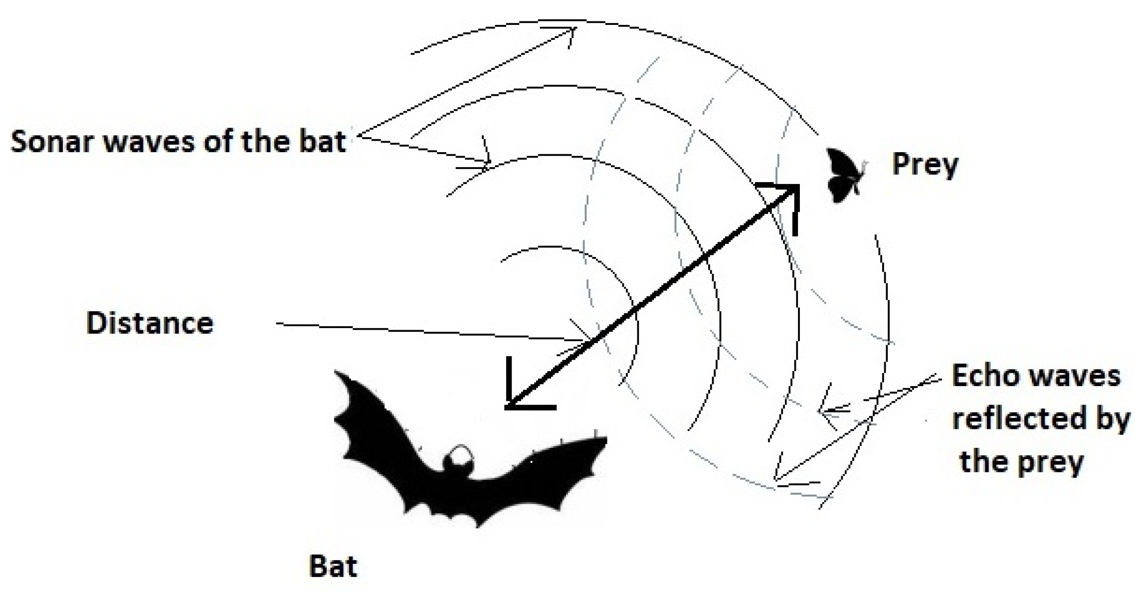Bat algorithm [35] is a promising metaheuristic for continuous optimization. Its metaphor is based on the echolocation behaviour of micro-bats, that can vary frequencies, loudness, and pulse rates of emission to capture the prey (see Figure 3).

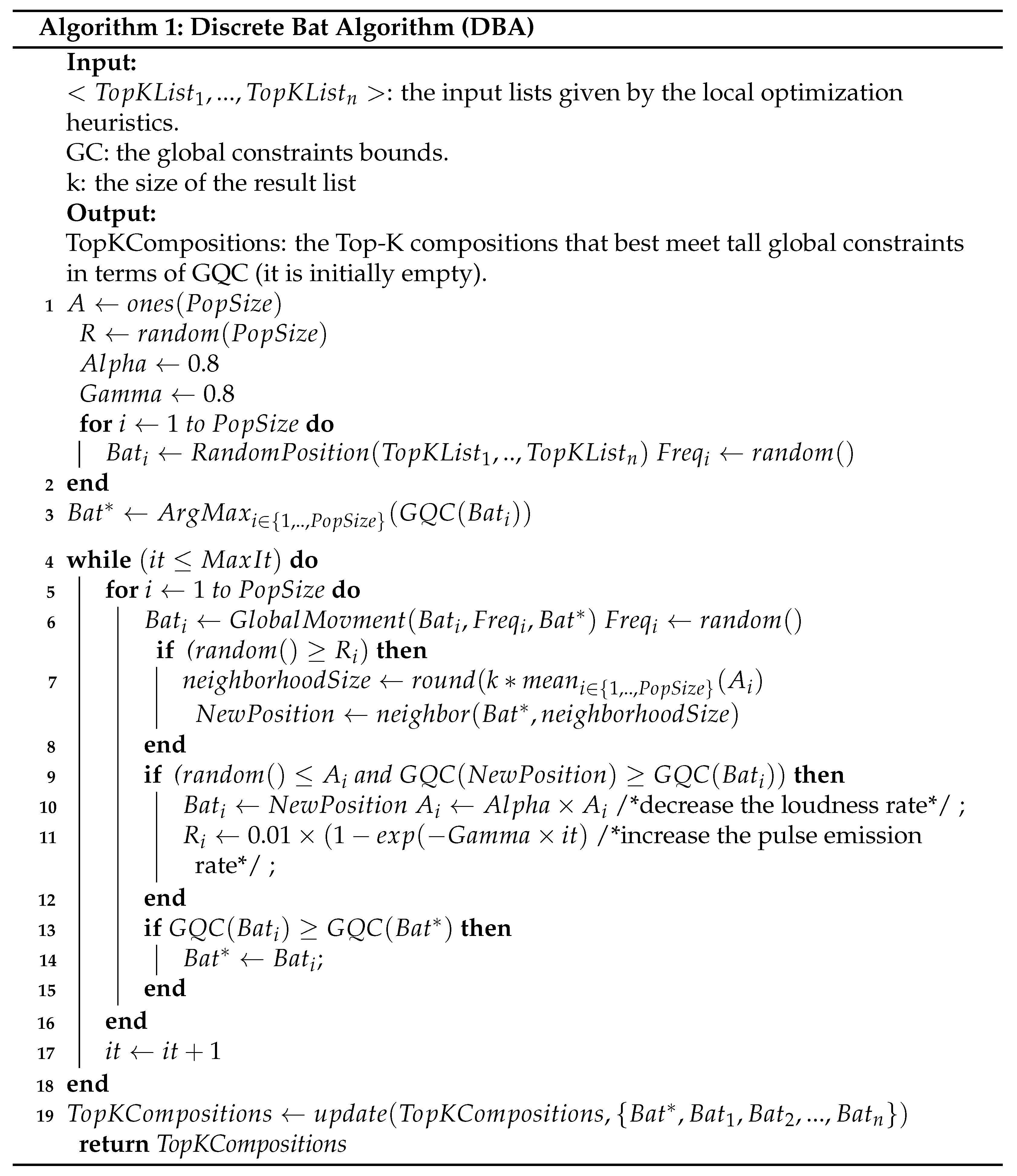
Before giving the pseudo-code of the discrete bat algorithm, we explain all its technical parameters.

Pop: it is a matrix of PopSize*n dimensions, it represents all the virtual bats.

P o p = {B a t_{1}, \dots, B a t_{P o p S i z e}}

B a t^{*}

: the position of the best bat.

A: it stands for the loudness of the chirp; it is a vector of Popsize random numbers comprised in [0,1], it controls the neighborhood size of the local search. It is decreased along the execution of the metaheuristic.

Freq: it stands for the frequencies of the bats. It is a matrix of PopSize*n dimensions, it controls the size of the moving step during the global search phase. It is initialized with random values between 0 and 1.

R: it stands for the pulse emission rate of each bat. Technically, it is a n-dimension vector of random numbers (in [0,1]) that controls the execution of the local search.

Alpha: the factor of decreasing A.

Gamma: it is a factor that controls the increasing rate of the pulse emission rate R.

MaxIt: the maximum number of iterations of DBA.

The pseudo-code of DBA can be explained as follows: Line 1 : for each bat, we initialize its loudness, pulse emission rate, and their updating rates Alpha and Gamma.

Line 2: for each bat, we randomly initialize its position and its frequency that it is used as a step displacement in the GlobalMovment (of line 6).

F r e q_{i}

is a real value belonging to [0,1].

Line 3: we compute the best bat position of the swarm in terms of GQC. we update the best bat position of the swarm.

Lines 4-18 : this is the principal loop of the metaheuristic; it is constituted of MaxIt iterations.

Lines 5-16 : this is the loop that explores all the bats.

Line 6: this function creates a new composition by moving toward the best solution with a random step. More specifically, for each component (task) j of a given bat i, we replace it with the corresponding value in

b a t^{*}

with a probability equal to

F r e q_{i} (j)

(

B a t_{i} (j) = B a t^{*} (j),

with a probability

= F r e q_{i} (j)

). The frequency of each bat is changed after that.

Line7:with a probabiity

1 - R_{i}

, we create a neighborhood centered on the best bat

B a t^{*}

The width of this neighborhood is equal to k times the average of all the possible loudnesses

A_{i}

(this width is termed as spread); then, we create a new composition NewPosition

= (c o m p o n e n t_{1}, \dots, c o m p o n e n t_{n})

as follows:

for each

j \in {1, \dots, n}

c o m p o n e n t_{j} = s u c c e s s o r_{T a s k_{j}} (B a t^{*} (j))

with a probability

= G a u s s i a n_{m e a n, σ} (| R a n k (B a t^{*} (j)) - R a n k (s u c c e s s o r_{T a s k_{j}} (B a t^{*} (j))) |)

. Knowing that

M e a n = R a n k (B a t^{*} (j))

and

σ = s p r e a d / 2

For instance, if a task j is constituted of the following ranked services

< S 9, S 15, S 4, S 20, S 2 >

, and we assume that

B a t^{*} (j) = S 4, m e a n = R a n k (B a t^{*} (j)) = 3

(it is ranked third in the list), and

σ = s p r e a d / 2 = 1

, then the neighborhood of S4, according to line 7, is equal to

{S 15, S 4, S 20}

. The probability of getting each of them as a value for

c o m p o n e n t_{j}

25 %, 50 %, 25 %

, respectively (since we approximate the Gaussian function for these three observations).

In lines 9-12, we accept the aforementioned solution NewPosition (i.e., we update

B a t_{i}

), with a probability

A_{i}

. In addition, NewPosition must have a fitness better than that of

B a t_{i}

We decrease the loudness

A_{i}

and increase the pulse emission rate

R_{i}

in order to reduce the chances of performing the local search in the future (i.e., line 7).

In lines 13-15, we update the best solution if the actual bat has a better fitness.

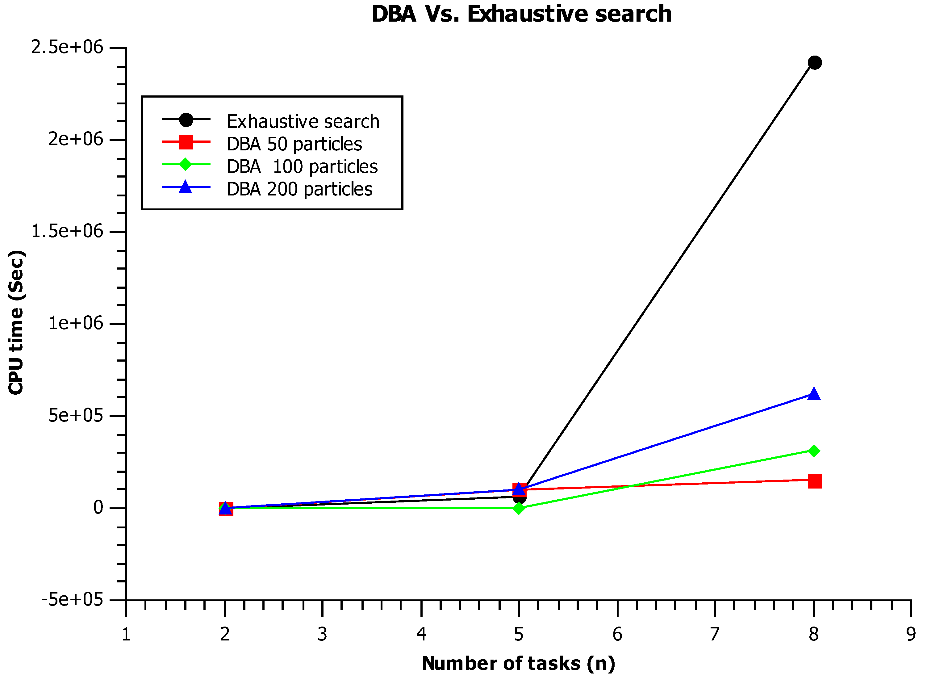
Finally, we notice that DBA has a time complexity of

O (P o p S i z e + n \times P o p S i z e + P o p S i z e \times r \times l^{n} + M a x i t \times P o p S i z e (n + n \times k + r \times l^{n}))

. We notice that the complexity of the fitness function GQC is

O (r \times l^{n}))

5. Experimental Study

Inspired from [3] and [25], we generate the QoS dataset using a random Gaussian distribution. In particular, we use the following setting: mean=0 and standard-deviation=1. The domain of each parameter is given in Table 3.

The experiments were implemented using a Window10 64 bit OS with Intel Core i3-6006U CPU @ 2.0GHz processor and 32 GB RAM. The algorithms where developed with netbeans IDE 12.0.

Before introducing the experimental results, we describe the theoretical complexity of the proposed heuristics. The heuristic H1 (Equation 15) compares each candidate service with the remaining components and each comparison step (Equation 13) is

O (r . l)

; therefore, the time complexity of H1 is

O (m . r . l)

. Like H1, the complexity of H2 (Equation 20) is

O (m . r . l)

. In the same line of thought, the complexity of Equation 24 (H3) is

O (m . r . l)

and the complexity of Equation 28 (H4) is

O (l . l o g l + m . r)

In the experiments, we will only vary one parameter and keep the remaining set to their default values (see Table 3). As regards the fuzzy dominance implementation of [21], we preserve the same setting chosen by the authors for the parameter

ε

(which is equal to 0.1). For the sake of concise presentation, we only show the Top2 pertinent compositions (in terms of GQC) for all the remaining experiments.

As shown in Figure 4, we observe that the behavior (time) of H1, H3, and the heuristic of (21) is comparable. Additionally, we observe a slight rise of time for H3 since the curve slope is proportional to

2 \times l

instead of l. At the end, we note that H2 and H4 are the most efficient heuristics since the slope of their curves is lower than the that of first ones.

The Figure 5 shows that the CPU time of H1, H3, and the heuristic of (21) is comparable, but the slopes of their respective curves are different. Additionally, we observe a slight rise of the time for the heuristic of (21) since its complexity is quadratic with respect to l. We note that H4 is the most efficient one since the comparison of median intervals does not depend on l (we assume that the sorting of QoS vectors is done in an offline way).

Like the previous experiments, Figure 6 shows that the fuzzy dominance implementation of (21), H1, and H3, have closer CPU times. On the other hand, the majority grade heuristic (28) and H4 have a lower CPU time since their theoretical slope is not dependent on l. We also note that the curve of H2 has an almost flat slope and this is mainly due to the low overhead of Equation 16. It is worth noting that, the majority grade principle is initially presented by [36] for ranking the candidates of an election. After that, it is adapted by [28] to web service selection.

According to Figure 7, we observe that all methods have almost the same CPU time up to n=5. Behind this threshold, the time rises with different scales (according to each alternative). We notice that the exhaustive search is the most prohibitive one since there is an exponential number of candidate solutions; however, DBA (with all configurations) only explores a polynomial number of candidate compositions (but GQC is still exponential). As a result, the increase rate of time is less drastic for the three configurations of DBA. In summary, we can state that a selection problem with less than 8 tasks can be efficiently handled with DBA while using less than 100 bats. It is worth noting that the majority of real-world workflows have less than 10 abstract tasks, and this fact highlights the suitability of DBA to the QoS aware service selection problem.

Figure 7. Average CPU time for DBA and Exhaustive Search.

Table 4. GQC and Global Constraints Satisfiability Vs. r.

	r=4		r=8		r=10
Model	GQC	PSGC	GQC	PSGC	GQC	PSGC
$H_{1}$	0.673	75%	0.484	50%	0.500	40%
	0.646	75%	0.480	62.5%	0.480	20%
$H_{2}$	0.721	100%	0.515	37.5%	0.570	30%
	0.664	100%	0.515	37.5%	0.463	30%
$H_{3}$	0.302	0%	0.393	0%	0.388	0%
	0.253	0%	0.343	0%	0.356	0%
$H_{4}$	0.562	50%	0.6628	12.5%	0.408	10%
	0.486	50%	0.524	25%	0.388	20%
Fuzzy dominance heuristic of (21)	0.673	75%	0.5155	37.5%	0.500	50%
	0.633	50%	0.515	50%	0.441	10%

Table 5 shows the behavior of the heuristics with respect to the QoS sample size l. Broadly speaking, we notice that both GQC and PSGC degrade as the l grows. This degradation is logic since the satisfaction of tight global constraints will be rare as l increases.We observe that H1 and H2 are more effective than the remaining heuristics; more specifically H2 performs better than H1 for low values of l (we can even obtain 100% of PSGC), however H1 performs better for medium and large values of l. In contrast to the heuristics H2, H3, and H4, we observe that H1 has a stable and consistent performance for all values of l.

Table 6 presents the performance of the heuristics with respect to m (the cardinal of the task). We observe a slight degradation for both GQC and PSGC when the number of services m increases, (for almost all heuristics). This observation may be due to the fact that the new extended dataset have less promising QoS levels. We also notice that the heuristics H1 and H2 are more effective than the rest of alternatives (for all values of m).

Table 7 demonstrates the performance of the heuristics with respect to the number of tasks n. It is clearly shown that the scores given by all heuristics degrade with the increasing of n, since it is more difficult to satisfy a constraint comprised of a larger sum of random variables (according to the central limit theorem, this sum will follow – under some conditions- a Gaussian probability distribution with a narrower standard deviation). Like the precedent experiments, we notice that H1 performs better than the rest of heuristic for all values of n. Additionnaly, we note that H2 has a better GQC and PSGC for low values of n, but these scores drastically degrade when n increases.

Table 8 presents a comparison between our contributions (DBA with H1 and H2) and some existing state-of-the-art approaches. It is clearly shown that GQC and PSGC of H1 and H2 are more effective than the works of the literature. We also observe that the work of [3] gives the lowest values for GQC, and this means that the methods based on local thresholds selection have worse performances on practical datasets. We also observe that the fuzzy implementation of the pareto-dominance using [33] is better than that of [21], since the experiments shown in Table 6, Table 5, Table 4 and Table 7 confirm the slight superiority of our proposed formula.

6. Conclusion

We have presented in this paper a set of ranking heuristics coupled with a bat algorithm metaheuristic for selecting service compositions with uncertain QoS. The main idea of the proposition consists of lowering the size space by first retaining the most pertinent services in each class (task) using well defined heuristics. In the second phase, we perform a global search to get the best compositions in terms of global QOS conformance. The results confirm the ability of both fuzzy pareto dominance relationship and stochastic dominance (of order zero) to outperform the remaining heuristics.

In future works, we plan to test the framework on other types of workflows and compare our bat algorithm method with recent metaheuristics such as Spider Monkey Optimization and whale optimization algorithm.

References

Hayyolalam V, Kazem AA. A systematic literature review on QoS-aware service composition and selection in cloud environment. Journal of Network and Computer Applications. 2018 May 15, 110:52-74.
Merzoug M, Etchiali A, Hadjila F, Bekkouche A. Effective Service Discovery based on Pertinence Probabilities Learning. International Journal of Advanced Computer Science and Applications. 2021,12(9).
Hwang, S. Y., Hsu, C. C., and Lee, C. H. Service selection for web services with probabilistic QoS. IEEE transactions on services computing, 2015,8(3): 467-480. [CrossRef]
Bekkouche, A., Benslimane, S. M., Huchard, M., Tibermacine, C., Hadjila, F., and Merzoug, M. QoS-aware optimal and automated semantic web service composition with user’s constraints. Service Oriented Computing and Applications, 2017. 11(2): 183-201.
Zhang S, Shao Y, Zhou L. Optimized artificial bee colony algorithm for web service composition problem. Int. J. Mach. Learn. Comput. 2021 Sep;11(5). [CrossRef]
Mohammed, M., Chikh, M. A., and Fethallah, H. QoS-aware web service selection based on harmony search. in IEEE ISKO-Maghreb: Concepts and Tools for knowledge Management (ISKO-Maghreb), 4th International Symposium , 2014, pp. 1-6.
Alrifai, M., Risse, T., and Nejdl, W. A hybrid approach for efficient Web service composition with end-to-end QoS constraints. ACM Transactions on the Web (TWEB),2012, 6(2): p7.
Liu, Z. Z., Jia, Z. P., Xue, X., An, J. Y. Reliable Web service composition based on QoS dynamic prediction. Soft Computing, 2015, 19: 1409-1425.
Belouaar, H., Kazar, O., and Rezeg, K. Web service selection based on TOPSIS algorithm. in 2017 IEEE International Conference on Mathematics and Information Technology (ICMIT),2017. pp. 177-182.
Shetty, J., D’Mello, D. A. Global and local optimisation-based hybrid approach for cloud service composition. in International Journal of Computational Science and Engineering,2018, 17(1): 1-14. [CrossRef]
Chen, L., Ha, W. Reliability prediction and QoS selection for web service composition. In International Journal of Computational Science and Engineering,2018, 16(2): 202-211.
Halfaoui A, Hadjila F, Didi F. QoS-aware web services selection based on fuzzy dominance. InComputer Science and Its Applications: 5th IFIP TC 5 International Conference, CIIA 2015, Saida, Algeria, May 20-21, 2015, Proceedings 5 2015 (pp. 291-300). Springer International Publishing.
Halfaoui, A., Hadjila, F., et Didi, F. QoS-aware web service selection based on self-organising migrating algorithm and fuzzy dominance. International Journal of Computational Science and Engineering, 2018, 17(4): p. 377-389.
Dahan F, El Hindi K, Ghoneim A, Alsalman H. An enhanced ant colony optimization based algorithm to solve QoS-aware web service composition. Ieee Access. 2021,9(2021):34098-111.
Zanbouri K, Jafari Navimipour N. A cloud service composition method using a trust-based clustering algorithm and honeybee mating optimization algorithm. International Journal of Communication Systems, 2020,33(5):e4259.
Zhu, W., Yin, B., Gong, S., Cai, K. Y. An Approach to Web Services Selection for Multiple Users, 2017, IEEE Access, 5:15093-15104. [CrossRef]
Yu, Q., and Bouguettaya, A. Computing service skyline from uncertain qows. IEEE Transactions on Services Computing, 2010, 3(1): 16-29. [CrossRef]
Schuller, D., Lampe, U., Eckert, J., Steinmetz, R., and Schulte, S. (2012, June). Cost-driven optimization of complex service-based workflows for stochastic QoS parameters. in 2012 IEEE 19th International Conference on Web Services (ICWS) ,2012, pp. 66-73.
Abdelhak E, Feth-Allah H, Mohammed M. QoS uncertainty handling for an efficient web service selection. InProceedings of the 9th International Conference on Information Systems and Technologies, 2019, pp. 1-7.
Brownlee J. A gentle introduction to the rectified linear unit (ReLU). Machine learning mastery. 2019 Jan 9;6.
Hadjila F, Belabed A, Merzoug M. Efficient web service selection with uncertain QoS. International Journal of Computational Science and Engineering. 2020, 21(3):470-82.
Rajeswari P, Jayashree K. Hybrid Metaheuristics Web Service Composition Model for QoS Aware Services. Comput. Syst. Sci. Eng.. 2022 Jan 1;41(2):511-24.
Sun, L., Wang, S., Li, J., Sun, Q., Yang, F. QoS uncertainty filtering for fast and reliable web service selection. In 2014 IEEE International Conference on Web Services, 2014, pp. 550-557.
Sun SX, Zhao J. A decomposition-based approach for service composition with global QoS guarantees. Information Sciences. 2012 Sep 15;199:138-53. [CrossRef]
Kim, M., Oh, B., Jung, J., and Lee, K. H. Outlier-robust web service selection based on a probabilistic QoS model. International Journal of Web and Grid Services, 2016, 12(2): 162-181.
Yasmina RZ, Fethallah H, Fedoua D. Selecting web service compositions under uncertain QoS. InComputational Intelligence and Its Applications: 6th IFIP TC 5 International Conference, CIIA 2018, Oran, Algeria, May 8-10, 2018, Proceedings 6 2018 (pp. 622-634). Springer International Publishing.
Seghir F, Khababa A, Semchedine F. An interval-based multi-objective artificial bee colony algorithm for solving the web service composition under uncertain QoS. The Journal of Supercomputing. 2019,75(2019):5622-66.
Zeyneb Yasmina R, Fethallah H, Fadoua L. Web service selection and composition based on uncertain quality of service. Concurrency and Computation: Practice and Experience. 2022.34(1):e6531.
Yasmina RZ, Fethallah H. Uncertain service selection using hesitant fuzzy sets and grey wolf optimisation. International Journal of Web Engineering and Technology. 2022,17(3):250-77.
Zheng, H., Zhao,W., Yang,J., Bouguettaya, A. QoS Analysis for Web Service Compositions with Complex Structures. IEEE Trans. Services Computing, 2013, 6(3): 373-386.
Benouaret, K., Benslimane, D., Hadjali, A. On the use of fuzzy dominance for computing service skyline based on qos. In 2011 IEEE International Conference on Web Services (ICWS), 2011, pp. 540-547.
Wang G, Jiang H. Fuzzy-dominance and its application in evolutionary many objective optimization. In IEEE 2007 International conference on computational intelligence and security workshops (CISW 2007), 2007,pp. 195-198.
Köppen M, Vicente-Garcia R, Nickolay B. Fuzzy-pareto-dominance and its application in evolutionary multi-objective optimization. InEvolutionary Multi-Criterion Optimization: Third International Conference, EMO 2005, Guanajuato, Mexico, March 9-11, 2005. Proceedings 3, 2005, pp. 399-412. Springer Berlin Heidelberg.
Bruni, R., Cesarone, F., Scozzari, A., Tardella, F. On exact and approximate stochastic dominance strategies for portfolio selection. European Journal of Operational Research, 2017, 259(1), 322-329.
Yang XS. A new metaheuristic bat-inspired algorithm. Nature inspired cooperative strategies for optimization (NICSO 2010). 2010:65-74.
Balinski M, Laraki R. A theory of measuring, electing, and ranking. Proceedings of the National Academy of Sciences. 2007 May 22,104(21):8720-5.

Figure 1. A general sequential workflow.

Figure 2. Service selection architecture.

Figure 3. Bat metaphor.

Figure 4. Average CPU time Vs. m.

Figure 5. Average CPU time Vs. l.

Figure 6. Average CPU time Vs. r.

Table 1. Motivating Example.

G.C: $AggregatedQoS (S_{x}, S_{y}) \geq 45$
Task T1	Task T2
$S_{1} :$	$S_{9} :$
$Q o S (S_{1}) = < 5, 15, 20, 30, 70 >$	$Q o S (S_{9}) = < 10, 11, 15, 20, 22 >$
$S_{2} :$	$S_{10} :$
$Q o S (S_{2}) = < 6, 18, 20, 40, 90 >$	$Q o S (S_{10}) = < 15, 18, 26, 30, 40 >$
$S_{3} :$	$S_{13} :$
$Q o S (S_{3}) = < 4, 15, 18, 25, 250 >$	$Q o S (S_{13}) = < 3, 8, 10, 20, 30 >$

Table 2. Notations.

Parameter	Semantic
n	The number of Tasks (classes).
m	The number of services per task.
r	The number of QoS Criteria.
l	The number of QoS realizations (i.e., or the sample size).
cl₁, cl₂,...,cl_n	The set of Tasks, each tasks involves atomic SaaS services with the same functionality and different QoS.
s₁ (resp. s₂,...,s_m)	represents the id of the selected service related to cl₁ (resp. $c l_{2}$ ,...,cl_n)
${QoS}_{p i j u}$	The value of the p^th QoS attribute related to the u^th instance of the service S_i $\in c l_{j}$ .
b₁,b₂,..b_r	The user’s global constraints (i.e., the bounds that need to be satisfied by the QoS of the composition).
w₁,..w_r	The weight of the QoS attributes, the default value of each w_p is $\frac{1}{r}$ .
k	The size of the outcome list (of compositions).

Table 3. Parameters’ Range.

Parameter	Meaning	Domain	Default value
n	The number of tasks	{2,5,8}	2
m	The number of services per class	{500,..,1000}	500
r	The number of QoS attributes	{4,..,10}	4
l	The number of realizations of a given QoS attribute (i.e., the number of instances)	{15,..,100}	21
k	The size of the returned list	{2,5,10}	5
$b_{i}$	The $i^{t h}$ global constraint bound	Positive real	For attributes aggregated with: an additive function: n*0.6.a multiplicative function: $0 . 6^{n}$ .MAX/MIN functions: 0.6.
$w_{i}$	The weight of the $i^{t h}$ QoS attribute	[0..1]	1/r

Table 5. GQC and Global Constraints Satisfiability Vs. l.

	l=15		l=21		l=100
Model	GQC	PSGC	GQC	PSGC	GQC	PSGC
$H_{1}$	0.673	75%	0.655	100%	0.420	0%
	0.646	75%	0.544	50%	0.414	0%
$H_{2}$	0.721	100%	0.704	50%	0.408	0%
	0.664	100%	0.655	100%	0.402	0%
$H_{3}$	0.302	0%	0.343	0%	0.346	0%
	0.253	0%	0.311	0%	0.324	0%
$H_{4}$	0.562	50%	0.538	25%	0.392	0%
	0.486	50%	0.467	25%	0.390	0%
Fuzzy dominance heuristic of (21)	0.673	75%	0.665	75%	0.415	0%
	0.633	50%	0.588	75%	0.411	0%

Table 6. GQC and Global Constraints Satisfiability Vs. m.

	m=500		m=800		m=1000
Model	GQC	PSGC	GQC	PSGC	GQC	PSGC
$H_{1}$	0.673	75%	0.645	75%	0.549	50%
	0.646	75%	0.626	75%	0.491	25%
$H_{2}$	0.721	100%	0.604	50%	0.552	50%
	0.664	100%	0.583	75%	0.486	75%
$H_{3}$	0.302	0%	0.358	0%	0.379	0%
	0.253	0%	0.311	0%	0.299	0%
$H_{4}$	0.562	50%	0.638	50%	0.506	25%
	0.486	50%	0.620	25%	0.474	25%
Fuzzy dominance heuristic of (21)	0.673	75%	0.590	75%	0.551	50%
	0.633	50%	0.583	75%	0.551	50%

Table 7. GQC and Global Constraints Satisfiability Vs. n.

	n=2		n=5		n=8
Model	GQC	PSGC	GQC	PSGC	GQC	PSGC
$H_{1}$	0.673	75%	0.665	50%	0.609	50%
	0.646	75%	0.656	50%	0.592	75%
$H_{2}$	0.721	100%	0.647	75%	0.224	0%
	0.664	100%	0.640	50%	0.219	0%
$H_{3}$	0.302	0%	0.163	0%	0.132	0%
	0.253	0%	0.161	0%	0.126	0%
$H_{4}$	0.562	50%	0.557	25%	0.512	25%
	0.486	50%	0.541	25%	0.511	25%
Fuzzy dominance heuristic of (21)	0.673	75%	0.563	50%	0.590	50%
	0.633	50%	0.557	50%	0.580	50%

Table 8. Utility Score, Global Constraints Satisfiability, and GQC for all methods (default configuration).

Heuristic	GQC	US	PSGC
$H_{1}$	0.655	0.531	75%
	0.544	0.482	100%
$H_{2}$	0.704	0.511	50%
	0.655	0.531	100%
$H_{3}$	0.342	0.387	0%
	0.311	0.374	0%
$H_{4}$	0.538	0.451	25%
	0.467	0.427	25%
Majority grade with constraint programming (28)	0.703	0.519	75%
	0.631	0.527	75%
Fuzzy dominance heuristic of (21)	0.665	0.516	75%
	0.588	0.514	75%
First assignment of (3)	0.302	0.398	0%

Disclaimer/Publisher’s Note: The statements, opinions and data contained in all publications are solely those of the individual author(s) and contributor(s) and not of MDPI and/or the editor(s). MDPI and/or the editor(s) disclaim responsibility for any injury to people or property resulting from any ideas, methods, instructions or products referred to in the content.

© 2023 by the authors. Licensee MDPI, Basel, Switzerland. This article is an open access article distributed under the terms and conditions of the Creative Commons Attribution (CC BY) license (http://creativecommons.org/licenses/by/4.0/).

Copyright: This open access article is published under a Creative Commons CC BY 4.0 license, which permit the free download, distribution, and reuse, provided that the author and preprint are cited in any reuse.

MDPI Initiatives

Important Links

Choose an area of interest and we will send you notifications of new preprints at your preferred frequency.

Disclaimer

An Intelligent Bat Algorithm for Web Service Selection with QoS Uncertainty

Abstract

1. Introduction

2. State of the Art

2.1. Service Selection with Certain QoS

2.2. Service Selection with Uncertain QoS

3. Problem Specification

3.1. Parameters’ Notation

3.2. QoS model

3.3. Global QoS Conformance

4. Proposed Approach

4.1. Overall Architecture

4.2. Local Optimization

4.2.1. Fuzzy Pareto Dominance Heuristic (H1)

4.2.2. Zero Order Stochastic Dominance (H2)

4.2.3. First Order Stochastic Dominance (H3)

4.2.4. Majority Interval Dominance (H4)

4.3. Global Optimization

5. Experimental Study

6. Conclusion

References

MDPI Initiatives

Important Links

Subscribe