Development of a Lux Meter for the Identification of Liquids in Post-Consumer Polyethylene Terephthalate Bottles for Collection Centers in Mexico

Preprint

Article

Development of a Lux Meter for the Identification of Liquids in Post-Consumer Polyethylene Terephthalate Bottles for Collection Centers in Mexico

Altmetrics

Downloads

Views

Comments

A peer-reviewed article of this preprint also exists.

L. Ángeles-Hurtado^‡

Juvenal Rodríguez^*,‡

,Hilda Romero-Zepeda^‡,H. Torres-Salinas^‡

R. García-Martínez^‡

Silvia Salas-Aguilar^‡

L. Ángeles-Hurtado^‡

Juvenal Rodríguez^*,‡

,Hilda Romero-Zepeda^‡,H. Torres-Salinas^‡

R. García-Martínez^‡

Silvia Salas-Aguilar^‡

^‡ These authors contributed equally to this work.

This version is not peer-reviewed

Submitted:

01 June 2023

Posted:

02 June 2023

You are already at the latest version

Alerts

Abstract

This article seeks to strengthen efforts in technological developments based on the classification of PET plastic that positively impacts sustainable development and contributes to suitable solutions in collection centers in Mexico. Three experiment designs and machine learning tools for data processing were developed. For the experimentation, three factors were considered: the bottle's size, the amount of liquids inside the bottle, and the label on the bottle. The first experiment was to identify the distance of the sensor from post-consumer PET bottles. The second experiment was to determine the detection ability of the sensor with different levels of liquids inside the bottles, and the third was to determine the detection ability on the bottle labels. A digital lux meter on a microcontroller was developed to monitor illuminance on post-consumer PET plastic when it contains liquid as it passes through a conveyor belt for processing at an average rate of three bottles per second. With the implemented methodology, liquids were satisfactorily detected inside the transparent PET bottles when they had beverages between 25% and 100% of their capacity. Finally, this paper highlights that it is possible to implement an affordable design to identify bottles with liquids for collection centers.

Keywords:

Subject: Engineering - Control and Systems Engineering

1. Introduction

Millions of metric tons of plastic are produced in the world every year. These tons represent a problem in managing urban and industrial solid waste. Initiatives are being developed worldwide to promote a recycling culture and thus reduce waste generation [1]. Polymers that can be recycled must have specific quality characteristics for processing [2]. In the United Mexican States, more than 86,343 tons of solid and organic waste are collected daily in homes, buildings, streets, avenues, parks, and gardens. More than half of these generated materials nationwide are organized in seven states. In Mexico, less than 11% of the garbage collected is separated daily [3]. The country has collection centers (CC) for urban solid waste. In the various CC where recyclable materials are purchased, users bring the bottles to be paid at a reasonable price. Still, they are contaminated inside and out with liquids or organic materials. Currently, a record of 501 CC collects various materials daily, of which 65% is paper, cardboard, PET, and glass. The states with the most CC are Ciudad de México with 411, Estado de México with 17, Hidalgo with 15, Quintana Roo with 15, and Aguascalientes with 11 [4]. In Mexico, 87 out of 100 people between 18 and 65 are interested in caring for the environment, but only 31 practice it [4,5]. Efficient separation and recovery of urban waste can lead to stopping carrying tons in the landfill, equivalent to months of life of the landfill [6]. For this reason, encouraging and facilitating people to reuse and recycle could impact the environment. Solid urban waste requires viable actions to transfer value to the final consumer and thus reduce the environmental impact. Some companies are leaders in Mexico and Latin America, providing direct employment for around 98 thousand people and generating more than one million indirect jobs to process recyclable plastics [7]. Daily, CC buy recyclable materials from polymers, ferrous and non-ferrous metals, and electrical and electronic materials. For these materials to have a market value again, they must be adequately separated. Recyclable polymers must not be mixed with other polymers, liquids, oils, or other materials. To increase recycling, personnel who can identify the material that could still be used again are required. The identification of these bottles is made chiefly manually, which delays the classification time and increases the losses by being unable to detect the contaminated bottles. The more contaminated the bottle inside, the more weight increases. Therefore, identifying the bottles with the most liquid or other material is essential. The proper classification of recyclable materials in CC, mainly polymers, contributes to maintaining a circular economy and provides employment. The modernization of CC could increase its productivity and contribute to the better management of plastics in developing countries [3]. This project proposes a possible solution to micro-enterprises established as CC to estimate the liquids they buy instead of plastic. The development and design of a digital lux meter aim to monitor the reflectance in post-consumer PET bottles when liquids are inside the bottle. There are commercial lux meters, but they are not designed for this purpose. It is proposed to provide an affordable alternative for its implementation that offers the advantage of generating actions after establishing a required value for the control in the amount of illuminance.

This paper aims to develop an automatic liquid identification system for recyclable polyethylene terephthalate bottles with an affordable design.
A new methodology is developed and implemented to identify dark liquids.
In conclusion, it is possible to quantify the number of dark liquids that post-consumer PET bottles can have by implementing an affordable design.

2. Methodology

Figure 1 summarizes the implemented methodology; it can be seen that the results of each stage are used for the final proposal.

2.1. Post-Consumer PET Bottles

Recyclable plastics (thermoplastics) are defined as polymers that can be melted and shaped almost indefinitely. They melt when heated and harden when cold; however, if frozen, thermoplastics can break, just like glass. These characteristics, to which they owe their name, are reversible so that the material can be heated, shaped, and frozen many times [8]. There are more than 100 types of plastics, six of which are the most used [9], and those that are most recycled: polypropylene, polyethylene, polyvinyl chloride, polystyrene, polyethylene terephthalate, and polycarbonate [10]. 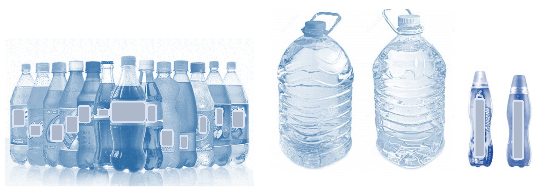They are identified by a number within a triangle that facilitates their identification and were codified by the Plastics Industrial Society in 1980 [11]. There are various presentations of PET bottles; see Figure 2.

PET bottles are identified by the number one within a triangular symbol often engraved on the bottom of the bottle. One million plastic bottles are sold worldwide every minute, and 60 million metric tons of PET are produced yearly. For soft drink manufacturers Coca-Cola and PepsiCo, the production of PET bottles from 250 milliliters to 600 milliliters constitutes 50% of annual sales. Bottling represents 30% of world PET production, 20 million metric tons. The annual consumption was estimated to exceed half a billion in 2021 [12]. Once the PET has been collected and classified, it represents a raw material for the recovery processing lines. The recovery involves washing the materials, mainly bottles, and conditioning the plastics to be processed as resin [13]. Because PET is food safe, it is used throughout the food delivery system. 50% of total plastic production is for single-use products [12]. Plastic waste has physical characteristics that comprise only 7% to 9% by weight and 20% to 30% by volume, respectively; this means that a lot of energy is required to store, move and process the waste polymers [14]. Despite these implications, recycling is profitable. Recycled PET can make fibers for carpets, clothing, 3D printer filaments, bags, toys, and other bottles. In Mexico, there are already 100% recycled bottles on the market, according to Coca-Cola. Recycling is essential to maintain an economic cycle but it also affects the environment. For example, PET bottles in landfills release and disperse more than 1,108 tons of antimony into the hydrosphere, pedosphere, and atmosphere, which can cause developmental disorders in children [15].

2.1.1. Physical Characteristics of Post-Consumer PET Bottles

For a post-consumer PET bottle to be a candidate for mechanical recycling, specific criteria are required, and it is even necessary to know the origin of the plastic to guarantee the purity of the resin. Plastics mainly come from the mass of urban solid waste from two prominent sources. These can be divided into three classes: those that have been classified and separated from each other from other classes; mixed waste: those of the same class but of a different color of cap or bottle. And mixed plastic waste combined with other debris: paper, cardboard, metal, etc., including plastics found in electronic waste. Among these types of bottles, the plastic in the PET bottle differs from the plastic screw cap used to seal them. Lids are generally high-density polyethylene or polypropylene, and the bottom of the lid is foamed polypropylene. This plastic is more rigid and has a higher melting point than PET [12].

2.1.2. Reducing the Problem to an Empirical Level

The growth of the population worldwide and the arrival of COVID-19 increased the use of single-use plastics and solid waste, mainly in cities [16]. There are at least 23 different presentations of PET bottles in Mexico, and their storage capacity ranges from 100 milliliters to more than 10 liters. Therefore, more efficient systems and methods are required to collect, classify, store, and process solids after having finished their life cycle. Solid waste collection and sorting of post-consumer recyclable materials require many resources and human resources. Developing automated systems that perform these activities reduces resources and labor. CC buys materials to be separated, classified, or treated for reuse; see Table 1. The modernization of CC in managing urban solid waste represents an economic, social, technological, and ecological opportunity.

By the method of observation and statistical analysis, this research work was carried out. The study contemplates only the characteristics of post-consumer PET bottles collected and taken to a CC for purchase. The study and data collection were conducted in Querétaro, in a CC called Materiales Reciclables Ángeles located north of the town. The data acquisition period was March 7, 2021, and the analysis ended May 6, 2023. An average of three people manually classified the collection of post-consumer PET bottles with prior knowledge of the characteristics that the post-consumer PET polymer must have to be recyclable. In the CC, it was decided to take a sample of 100 kg of post-consumer PET bottles considering the post-consumer physical characteristics to approximate the number of liquids in the sample. Four thousand nine hundred and fifty-nine post-consumer PET bottles were the sample studied. The bottles were unsorted and of various sizes and colors.

2.2. Materials

For the experimentation, various materials were used to automate the experiment and minimize the variation of the data, thus avoiding external factors such as the environment, etc.

2.2.1. Mechanical Design Parameters

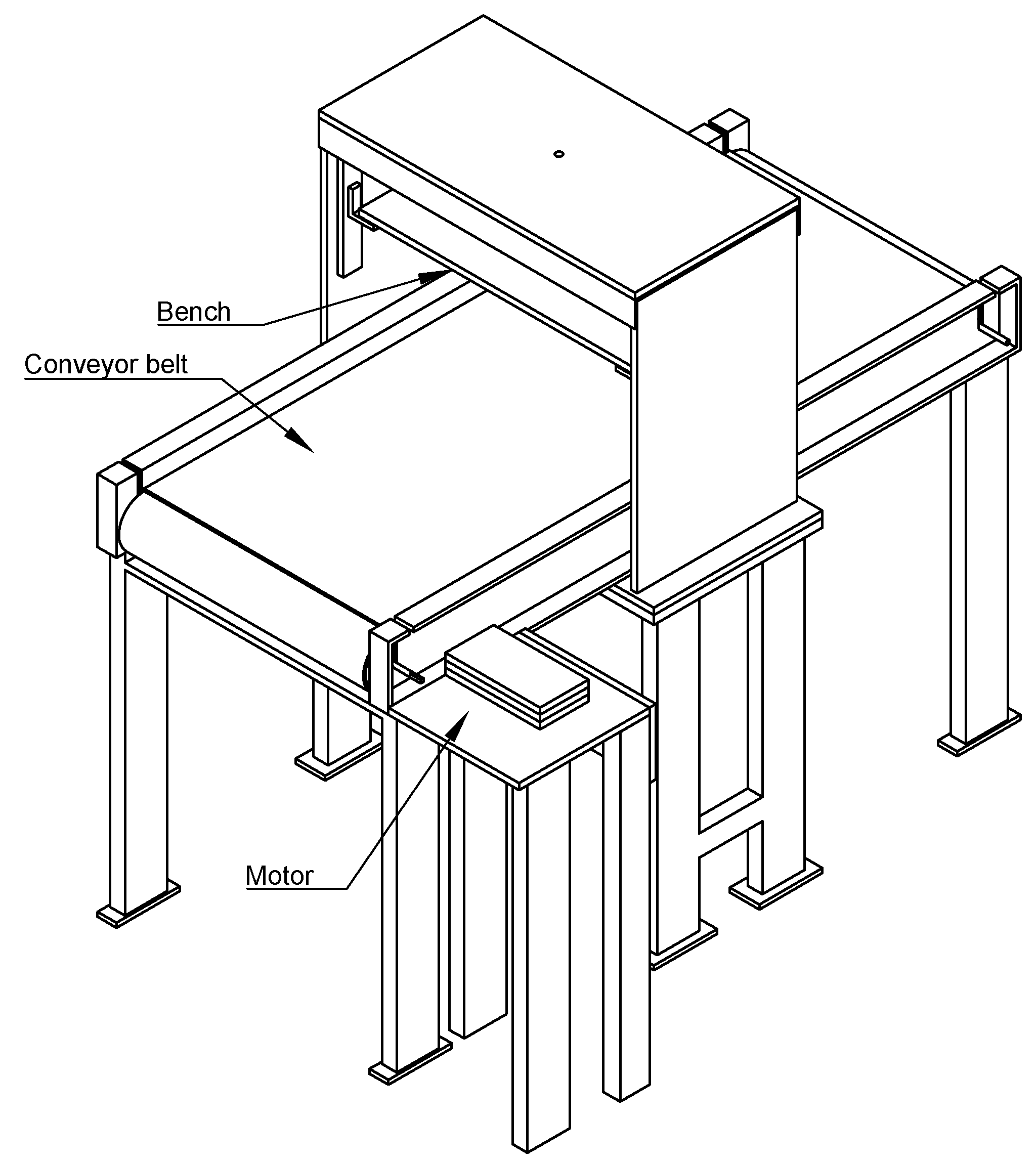
For experimentation, a mechanical system was developed to transport bottles of different sizes; the design parameters can be seen in Table 2. A conveyor belt and a mobile structure were used to determine the best position for data acquisition to assemble the lux meter. The conveyor belt has a geared motor with 1750 revolutions per minute and a reducer of one hundred to one, equivalent to making eighteen turns in one minute.

2.2.2. Electronic Card

Table 3 shows part of the materials used to develop the lux meter.

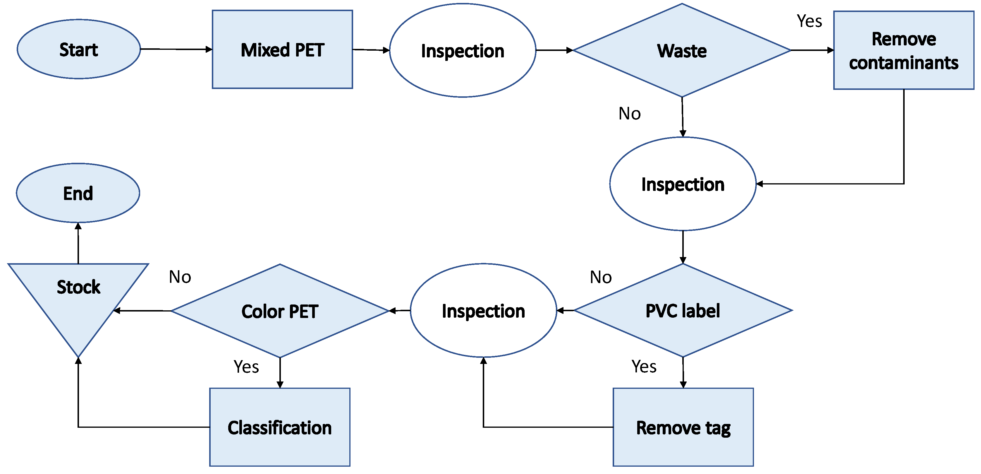
2.3. Description of the Manual Bottle Classification Process

Figure 3 describes the process used in the study to discriminate post-consumer PET bottles. The experimentation began in the company CC Recyclable Materials Angeles. The material purchased is mixed, so it is inspected to find out what conditions it is in. It is also considered if the bottle has a label and is removed depending on whether it covers the entire bottle; then, it is classified according to the color of the bottle; finally, it is compacted and stored.

From the 100 kg sample, it was expected to observe at least 23 different types of post-consumer PET bottles, considering liquid storage capacity as the main differentiator; bottles range from 100 milliliters to 10 liters. To verify that the sample had been representative, we used the information provided by the soft drink manufacturers Coca-Cola and PepsiCo. Which report that their production of PET bottles from 250 milliliters to 600 milliliters constitutes 50% of annual sales [12].

2.4. Design of Experiments for Variable Identification

Design of Experiments (DOE) is a practical statistical tool design and testing. DOE provides a sequential strategy to a region containing the optimum settings of the variables. Suppose a large number of variables can affect the performance of a system, but only a relatively small number of them are essential. In that case, a screening experiment can be conducted to identify the critical variables [17]. Three DOEs were developed, two with two factors and the other with only one factor. The distance, the size of the bottle, and the label of the bottles are factors that were considered to affect the illuminance measurement; see Table 4.

2.4.1. Design of Experiments to Determine the Distance and Working Range of the Lux Meter

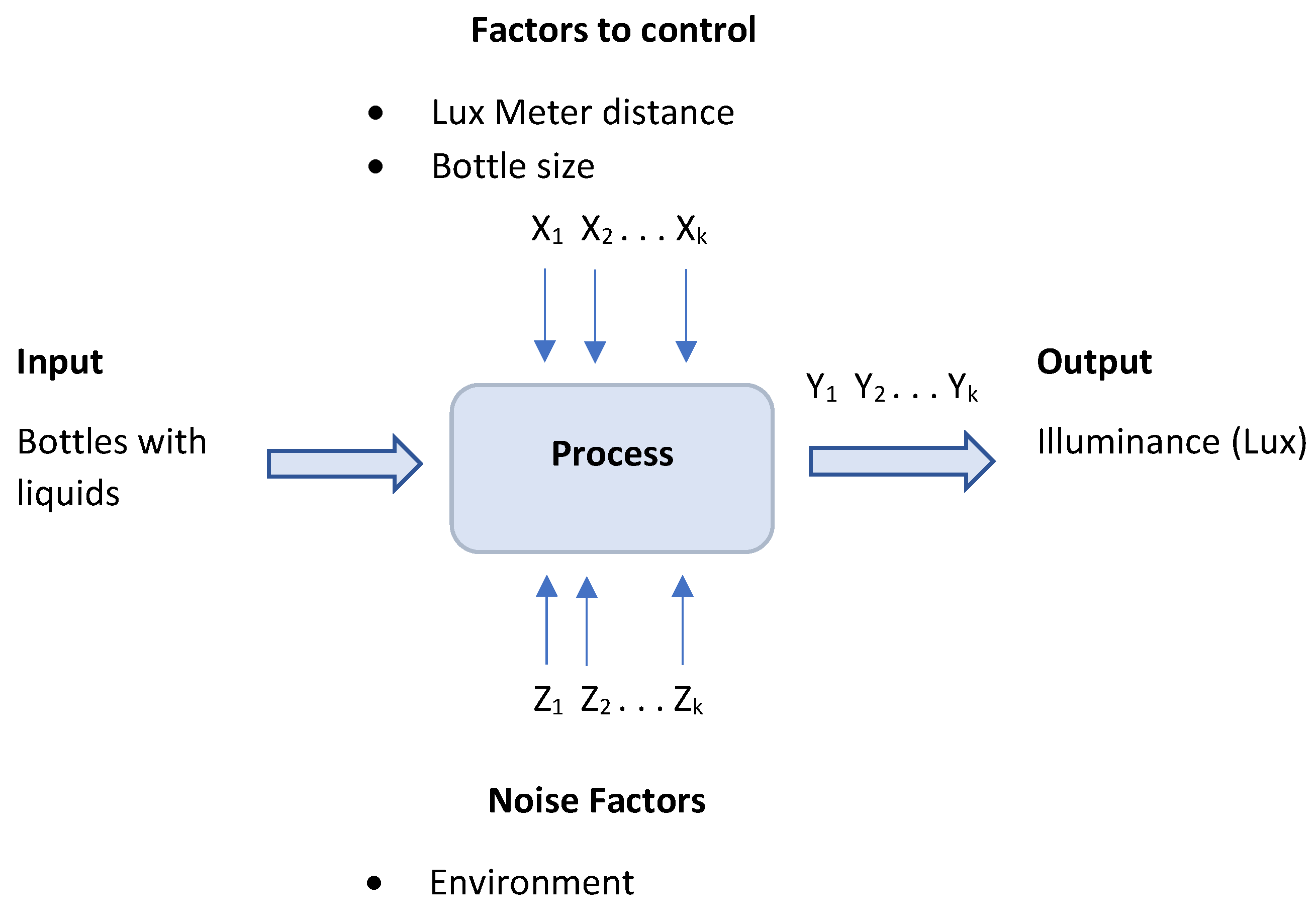
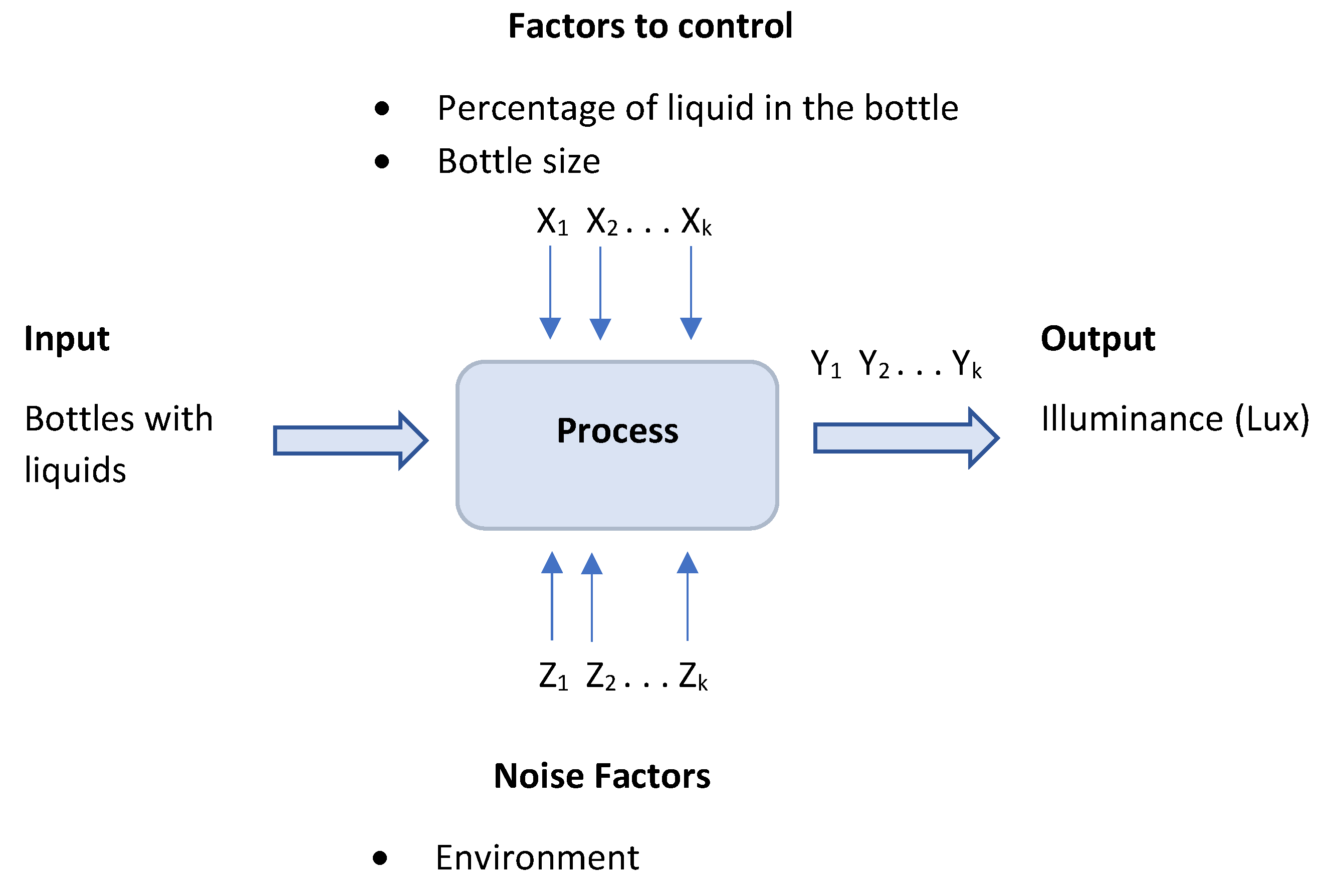
To determine the position of the lux meter, a DOE was developed that helped us obtain readings that represent the amount of liquid inside the bottles. Figure 4 illustrates the causality diagram with the considered factors; see Table 5.

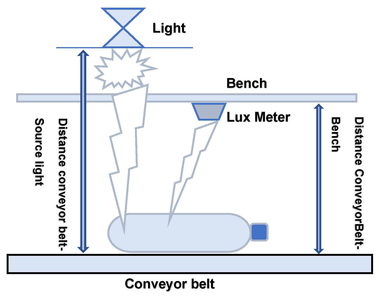
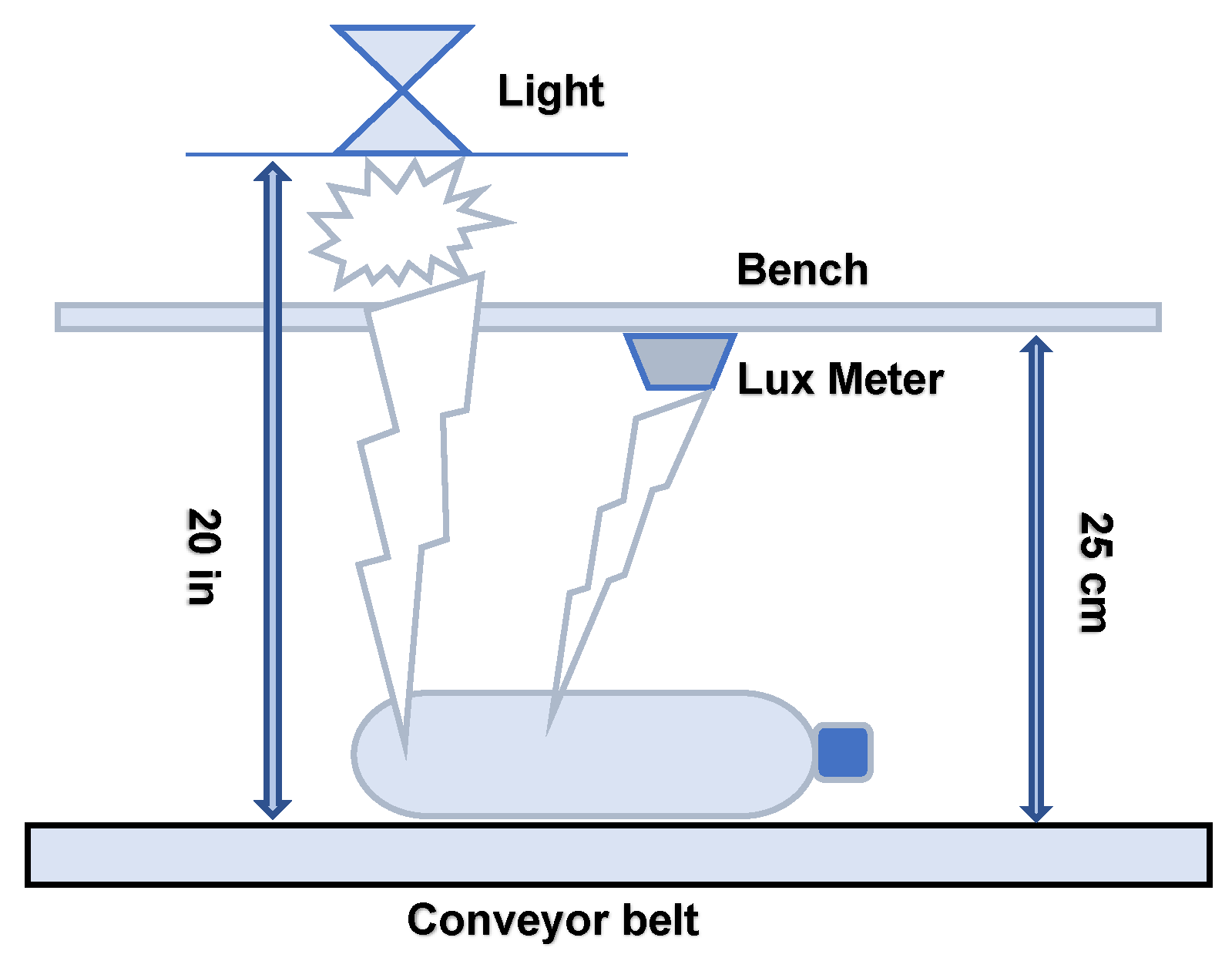
The position of the bottle was established vertically in the direction of the conveyor belt; it is essential to highlight that other positions were not considered. The experimentation was carried out with dark liquids; see Figure 5 to know the interaction of the distance factor [18]. With the data obtained, the significant distance was determined to determine the operating range of the lux meter.

Table 6 summarizes the results of the sources of variation of the preparation of the ANOVA of two factors.

2.4.2. Design of Experiments to Identify the Minimum Amount of Liquids Inside the Bottle

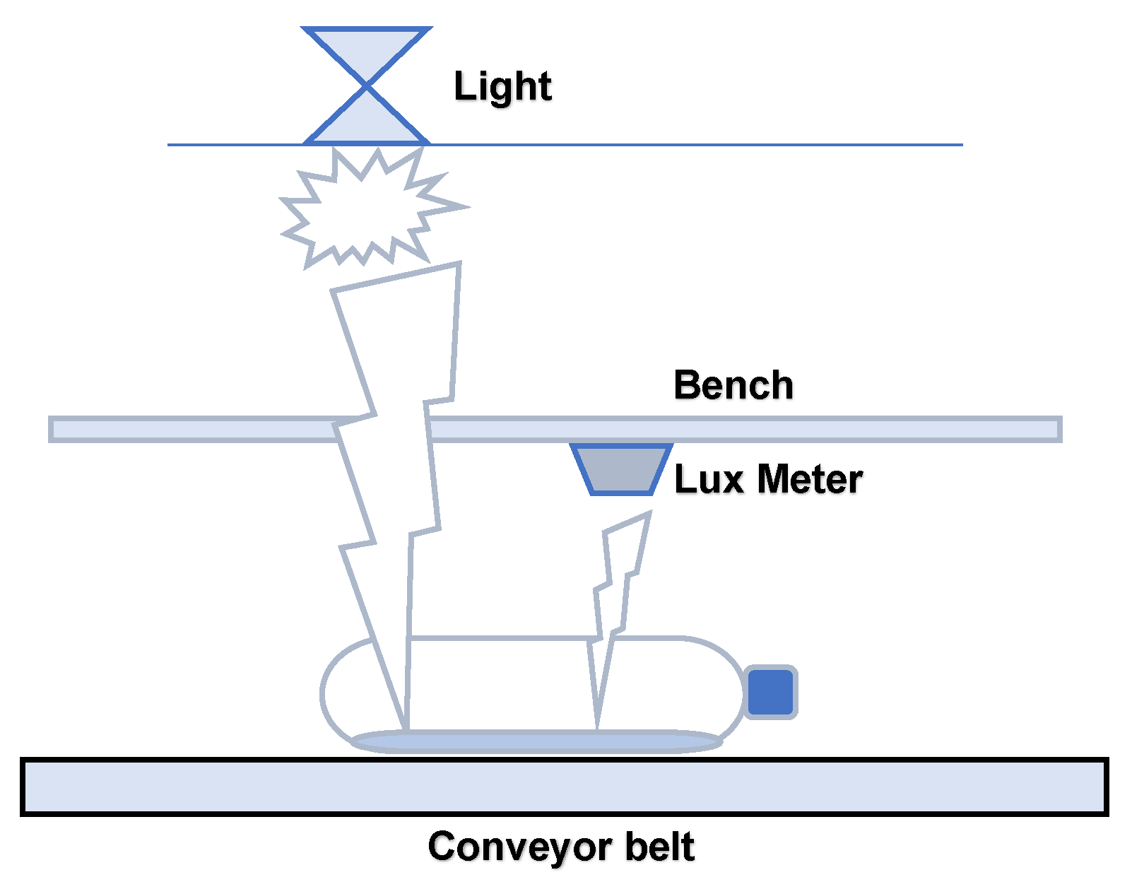
The distance was considered a fixed factor once the results of the first DOE were obtained. The second DOE was developed to obtain readings representing the minimum amount of liquid inside the bottles; see Table 7. The position of the bottle was maintained as in the first DOE; see Figure 6.

The minimum amount of liquids the lux meter could identify was determined with the data obtained. With the results of the two DOE, the minimum characteristics that the lux meter must have were established.

2.4.3. Design of Experiments to Determine Label Illuminance

A one-factor DOE was performed to identify the reflectance of the labels on the bottles. A recommendation to determine the number of replicates (n) is that the degrees of freedom of the error are at least 20 or 25. According to this recommendation, we use the double

N = a + 50

, where

n = N / a

, where a is the number of levels of factor A. For this example, considering a minimum of 50 degrees of freedom in error and

N = 10 + 50

n = 60 / 10

, so six replicates were performed. See Table 8 [19].

Table 9 summarizes the results of the sources of variation of the elaboration of the ANOVA of a fixed factor.

Once the three DOE were finished, their results were processed using principal component analysis. The results will help us identify and approximate the amount of liquids inside the bottle.

2.5. Principal Component Analysis

PCA is a numerical research method; its main objective is to explain the maximum variance with the least number of components. PCA can analyze the main elements of multiple characteristics, expose nature by highlighting its main features, and shorten the data dimensions to help diagnose complex problems. The first component represents the most significant percentage of the total variation in the data. The second component represents the second largest percentage of the total data variation, and so on [20,21]. Minitab 17 Statistical Software was used for this analysis. The PCA was used to describe the variation between the DOE results and their correlation, reducing the complexity and aiding the interpretation of the data.

2.6. Support Vector Machine

SVM has robust classification capability considering statistical learning theory and the principle of minimum structural risk, which effectively solves small-sample, high-dimensional, nonlinear learning problems and overcomes the shortcomings of network learning artificial neural that is difficult to determine the rational structure. SVM improves the generalizability of learning methods [20,22]. In general, SVM is a linear classifier for two data types, one of which is labeled as follows:

(x_{1}, y_{1})

,...,

(x_{l}, y_{l})

where

x_{i} \in R^{N}

is a feature vector and

y_{i} \in {- 1, 1}

is a label belonging to a class. An SVM constructs an optimal hyperplane as a surface decision to separate data points of two classes. The hyperplane margin is defined as the minimum distance from the hyperplane training points [23]. The learning problem of SVM is to search for the optimal hyper-plane once the data set is obtained, find the values of w and b such that they satisfy the condition:

y_{i} (w^{t} x_{i} + b) \geq 1

; i=1,2,...,l [24].

2.7. Development of the Lux Meter and Liquid Identification System

2.7.1. Definition of the Measurand for the Measurement of Illuminance

A system that works in the visible spectrum was developed to use the illuminance measurement; it can be identified if the liquid is inside the plastic bottle, see Figure 7. At this stage, a lux meter was developed that identifies a bottle with no deformation and a label [25].

The measurand is the electric current that passes through a silicon photo-diode for illuminance measurement. The measure is indirectly due to the properties of the sensor that, when the illuminance varies in the photo-diode, its resistance changes [26]. If the relationship between V and I is linear, we say that we are in the presence of an ohmic material or component. The relationship that describes this behavior is known as the law of Ohm,

I = \frac{V}{R}

. By varying the resistance of the photo-diode due to the change in illuminance and the induced V, the I will change; depending on this variation, the illuminance can be calculated. To illustrate the behavior of the sensor, the manufacturer provides information represented in [26], and it can be seen that the scale is logarithmic-logarithmic.

2.7.2. Ambient Light Sensor BPW21R

Illuminance measures the intensity of light incident on a surface and can be correlated to the brightness perceived by the human eye. In the visible range, it is measured in units called lux. Ambient light sensors detect light or brightness like the human eye. A standard silicon photodetector is more sensitive to infrared than visible light. Using BPW21R ambient light sensors will solve this problem because they are most sensitive to the visible part of the spectrum. On the other hand, there is a strictly logarithmic correlation between open circuit voltage and illumination over the same range. BPW21R is a planar PN silicon photodiode specially designed for high-precision linear applications. Due to its extremely high resistance to darkness, the short-circuit photocurrent is linear over seven decades of illumination level. The device has a flat glass window built with a color correction filter, approximating the human eye spectral response. A standard silicon photodetector is much more sensitive to infrared than visible light. By contrast, BPW21R is sensitive to the visible part of the spectrum [26,27]. This work has reduced incandescent light and sunlight for the exact lux measurement.

3. Results

This work considered that the plastics came from homes, apartments, condominiums, and commercial areas generated by retail businesses, offices, and hotels because the bottles presented less than 1% It should be noted that it was decided to round their value for the data capture of certain bottles that were very close in storage capacity. For example, the 1.75L bottles were added to the 2L bottles.

3.1. Sample Results of the Classification Process Manually

Four thousand nine hundred fifty-nine post-consumer PET bottles were analyzed, representing over 100 kg. The results can be seen in Table 10, and it can be seen that the bottle that presented the most is the 600 milliliter bottle with 26.35%. On the other hand, eight types of bottles represent 94% of the variation that could be had from the 23 bottles that were thought to be presented in the sample.

With the results, the characteristics of the 0.25 L, 0.35 L, 0.6 L, 0.5 L, 1 L, 1.5 L, 2 L, 3 L PET bottles are considered in the next stage. This means that by basing the experimentation on eight types of bottles, we could obtain an approximation of other kinds of bottles with similar characteristics.

3.2. Design of Experiments for Variable Identification

3.2.1. Design of Experiments to Determine the Distance and Working Range of the Lux Meter

The design of experiments with three different distances with zero speed on the conveyor belt was developed. The design experiments were carried out with a commercial lux meter to identify the distance the lux meter should have and to identify liquids inside the bottles.

A: Distance from the lux meter to the conveyor belt (20, 25, 30 centimeters).
B: Bottle Size (200, 300, 355, 500, 600, 1000, 1500, 2000, 3000 milliliters).

The initial conditions to start the experiment was to take the reading of the lux meter when the light source was off, and the lessons were

0.3 - 0.4

lux. Subsequently, the light source was turned on, and the light reflected from the conveyor belt was between

13.8 - 14.5

lux. For replicates and not repetitions to be considered in this experiment, they were developed at different times and on other days. The DOE implementation is shown in Table 11, and the results are in Table 12. In [19] mentions that for the case of two factors, it recommends that the minimum sample size is

N = a + b + (a - 1) (b - 1) + 24

; see Equation (1)

N = a + b + (a - 1) (b - 1) + 24 = 3 + 9 + (3 - 1) (9 - 1 + 24) = 52

(1)

The number of replicates per cell is

N / a b

, where a and b are, respectively, the number of levels of factors A and B. For this design, N is considered to be 54

n = N / a b = 54 / (3) (9) = 2 .

(2)

The following Equations (3) to (7) shows the elaboration of the ANOVA of two factors. The sum of squares and degrees of freedom was calculated as follows.

S S T = \sum \sum y_{i j}^{2} - \frac{{(\sum \sum y_{i j})}^{2}}{N} = {(13.4)}^{2} + \dots + {(16)}^{2} - \frac{771.6}{54} = 371.0533

(3)

S S A = \frac{\sum T o t a l S u m_{i}^{2}}{b n} - \frac{{(\sum \sum y_{i j})}^{2}}{N} = \frac{{(215.8)}^{2} + {(273.2)}^{2} + {(282.6)}^{2}}{18} - \frac{{(771.6)}^{2}}{54} = 145.2844

(4)

S S B = \frac{\sum T o t a l S u m_{j}^{2}}{a n} - \frac{{(\sum \sum y_{i j})}^{2}}{N} = \frac{{(88)}^{2} + \dots + {(79.9)}^{2}}{6} - \frac{{(771.6)}^{2}}{54} = 19.73

(5)

S S A B = \frac{\sum S u m_{i j}^{2}}{2} - \frac{{(\sum \sum y_{i j})}^{2}}{N} - S S A - S S B = \frac{{(26.1)}^{2} + \dots + {(33)}^{2}}{2} - \frac{{(771.6)}^{2}}{54} - 145.2844 - 19.73 = 194.5788

(6)

S S E = S S T - S S A - S S B - S S A B = 371.0533 - 145.2844 - 19.73 - 194.5788 = 11.46

(7)

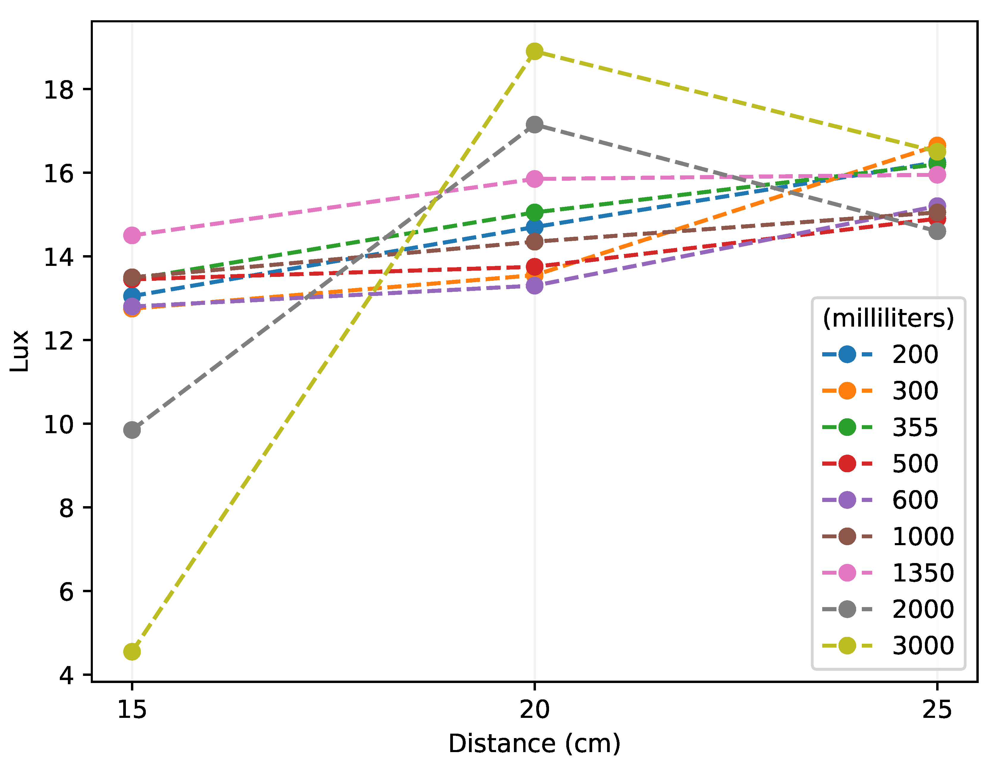
With the ANOVA we seek to know if the factors are significant and if there is an interaction. Interaction is defined as a dependency relationship between the value of the response and the levels of two or more variables. The response graphs are presented in Figure 8. His calculations are:

\begin{matrix} {\bar{Y}}_{A 1} & = \frac{215.8}{18} = 11.98 & {\bar{Y}}_{A 2} & = \frac{273.2}{18} = 15.17 & {\bar{Y}}_{A 3} & = \frac{282.6}{18} = 15.7 \\ {\bar{Y}}_{B 1} & = \frac{88}{6} = 14.66 & {\bar{Y}}_{B 2} & = \frac{85.9}{6} = 14.31 & {\bar{Y}}_{B 3} & = \frac{89.4}{6} = 14.9 \\ {\bar{Y}}_{B 4} & = \frac{84.2}{6} = 14.03 & {\bar{Y}}_{B 5} & = \frac{82.6}{6} = 13.76 & {\bar{Y}}_{B 6} & = \frac{85.8}{6} = 14.3 \\ {\bar{Y}}_{B 7} & = \frac{92.6}{6} = 15.43 & {\bar{Y}}_{B 8} & = \frac{83.2}{6} = 13.86 & {\bar{Y}}_{B 9} & = \frac{79.9}{6} = 13.31 \\ {\bar{Y}}_{A 1 B 1} & = \frac{26.1}{2} = 13.05 & {\bar{Y}}_{A 1 B 2} & = \frac{25.5}{2} = 12.75 & {\bar{Y}}_{A 1 B 3} & = \frac{26.9}{2} = 13.45 \\ {\bar{Y}}_{A 1 B 4} & = \frac{26.9}{2} = 13.45 & {\bar{Y}}_{A 1 B 5} & = \frac{25.6}{2} = 12.8 & {\bar{Y}}_{A 1 B 6} & = \frac{27}{2} = 13.5 \\ {\bar{Y}}_{A 1 B 7} & = \frac{29}{2} = 14.5 & {\bar{Y}}_{A 1 B 8} & = \frac{19.7}{2} = 9.85 & {\bar{Y}}_{A 1 B 9} & = \frac{9.1}{2} = 4.55 \\ {\bar{Y}}_{A 2 B 1} & = \frac{29.4}{2} = 14.7 & {\bar{Y}}_{A 2 B 2} & = \frac{27.1}{2} = 13.55 & {\bar{Y}}_{A 2 B 3} & = \frac{30.1}{2} = 15.05 \\ {\bar{Y}}_{A 2 B 4} & = \frac{27.5}{2} = 13.75 & {\bar{Y}}_{A 2 B 5} & = \frac{26.6}{2} = 13.3 & {\bar{Y}}_{A 2 B 6} & = \frac{28.7}{2} = 14.35 \\ {\bar{Y}}_{A 2 B 7} & = \frac{31.7}{2} = 15.85 & {\bar{Y}}_{A 2 B 8} & = \frac{34.3}{2} = 17.15 & {\bar{Y}}_{A 2 B 9} & = \frac{37.8}{2} = 18.9 \\ {\bar{Y}}_{A 3 B 1} & = \frac{32.5}{2} = 16.25 & {\bar{Y}}_{A 3 B 2} & = \frac{33.3}{2} = 16.65 & {\bar{Y}}_{A 3 B 3} & = \frac{32.4}{2} = 16.2 \\ {\bar{Y}}_{A 3 B 4} & = \frac{29.8}{2} = 14.9 & {\bar{Y}}_{A 3 B 5} & = \frac{30.4}{2} = 15.2 & {\bar{Y}}_{A 3 B 6} & = \frac{30.1}{2} = 15.05 \\ {\bar{Y}}_{A 3 B 7} & = \frac{31.9}{2} = 15.95 & {\bar{Y}}_{A 3 B 8} & = \frac{29.2}{2} = 14.6 & {\bar{Y}}_{A 3 B 9} & = \frac{33}{2} = 16.5 \end{matrix}

At a closer distance, the larger capacity bottles reflect less, and at a greater distance, the reflectance seems to stay between

14.7 - 16.5

lux. When comparing the initial conditions when there is no bottle on the conveyor belt, the range is between

13.8 - 14.5

. Therefore, it indicates that the illuminance increases when a bottle with liquid is between

0.9 - 2

lux.

The significant distance to obtain the illuminance was determined with the data obtained. Figure 9 shows the optimal distance between the conveyor belt and between the light source and the conveyor belt.

3.2.2. Design of Experiments to Identify the Minimum Amount of Liquids Inside the Bottle

The initial conditions to start the experiment was to take the reading of the lux meter when the light source was off, and the readings were between

0.7 - 0.8

lux. With the light source on, it is reflected between

15.6 - 17.8

lux. They were developed at different times and on other days for replicates and not repetitions to be considered in this experiment. The conveyor belt was cleaned, which caused an increase in reflectance, see Table 13 and Table 14 for see the results.

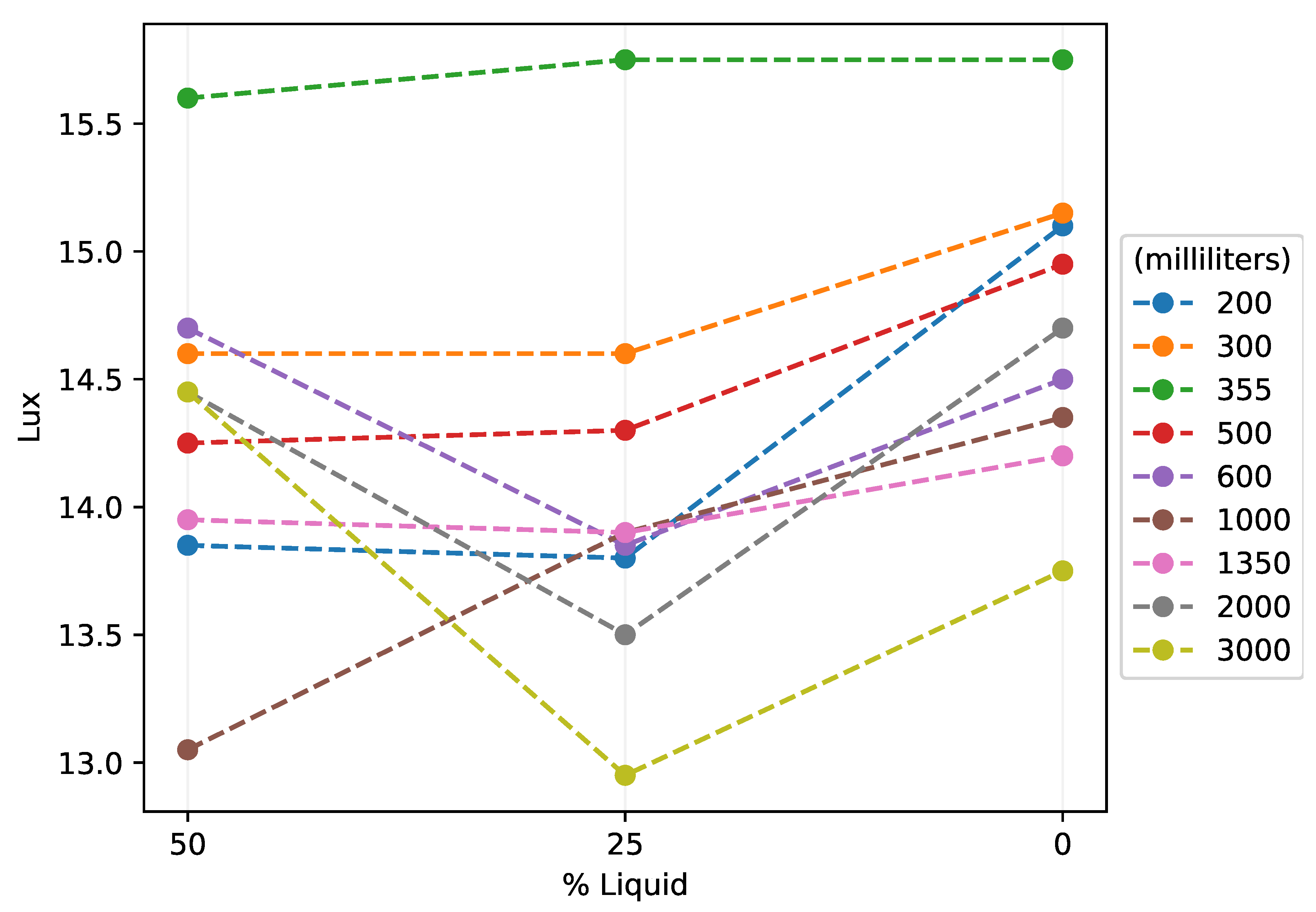
A: Percentage of liquids in the bottle (50, 25, 0 %).
B: Bottle Size (200, 300, 355, 500, 600, 1000, 1500, 2000, 3000 milliliters).

Figure 10 shows an interaction between the factors. And it describes that the less amount of liquid inside the bottle, the amount of illuminance increases depending on the size of the bottle. This means that the operating range is between

13.75 - 15.75

lux and that the variation in illuminance is between

1.85 - 2.05

lux.

3.2.3. Design of Experiments to Determine the Illuminance on the Labels

In the third DOE, it was considered that the label of each bottle is not uniform, so depending on its position, it would give a different reading, see Table 15.

The calculation of sums of squares and degrees of freedom for a factor is done as follows:

S S T = \sum \sum y_{i j}^{2} - \frac{{(\sum \sum y_{i j})}^{2}}{N} = {(30)}^{2} + \dots + {(18)}^{2} - \frac{{(1240.20)}^{2}}{60} = 804.526

(8)

S S t = \frac{\sum S u m_{j}^{2}}{n} - \frac{{(\sum \sum y_{i j})}^{2}}{N} = \frac{{(163.20)}^{2} + \dots + {(105.4)}^{2}}{6} - \frac{{(1240.20)}^{2}}{60} = 722.48

(9)

S S E = S S T - S S t = 804.526 - 722.48 = 82.046

(10)

g l (S S T) = N - 1 = 60 - 1 = 59

(11)

g l (S S t) = a - 1 = 10 - 1 = 9

(12)

g l (S S E) = g l (S S T) - g l (S S t) = N - a = 60 - 10 = 50

(13)

The results of the sums of squares and degrees of freedom calculations are shown in Table 16. With the results obtained, it is concluded that 48.92 is more significant than 2.07, and the equality of means is rejected. The size of the label affects the illuminance.

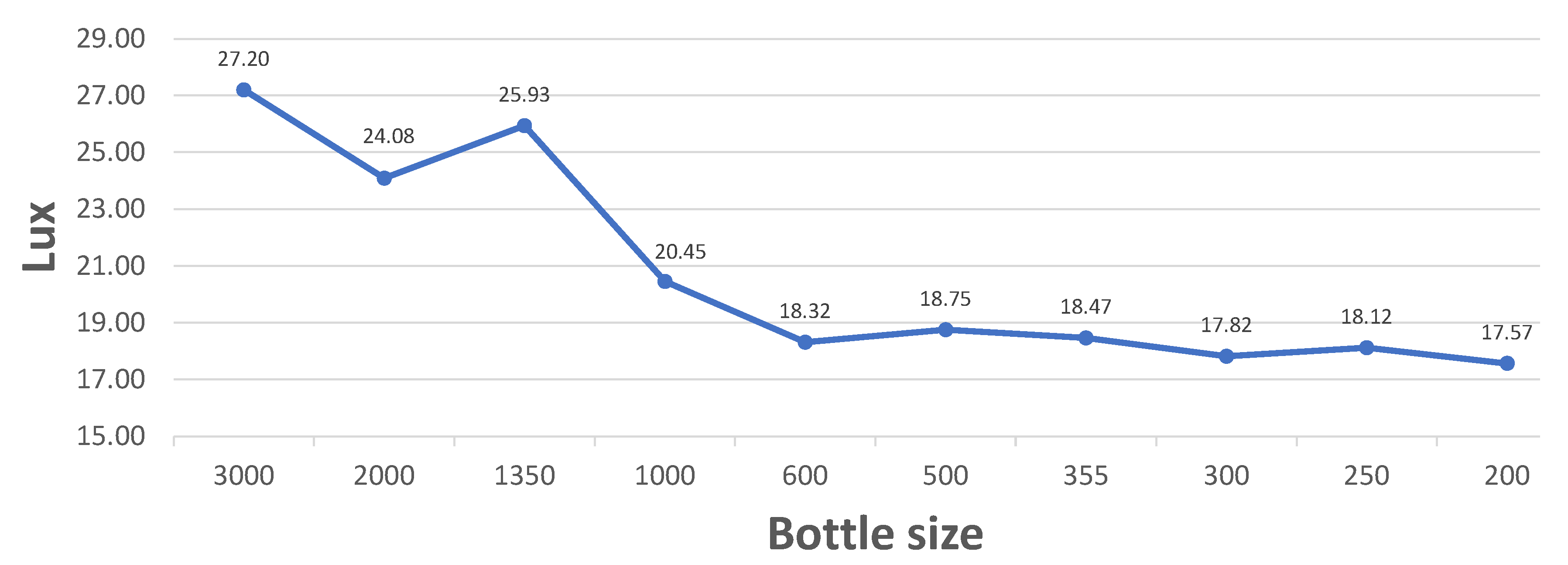
The experiment was done by modifying the bottle in different positions to obtain the most significant variation between replicates. In Figure 11, it is concluded that as the size of the label on the bottle decreases, the illuminance decreases. But the illuminance increases when the bottle has a label; this occurs when the brand has white letters.

3.3. Principal Component Analysis, PCA

Finally, principal component analysis was used to identify the number of liquids in the bottles. Data was entered into Minitab software, and the data and results are shown in Table 17.

Transforming the data with the following formula

x_{i j} = \frac{x_{i j} - {\bar{x}}_{j}}{σ_{j}}

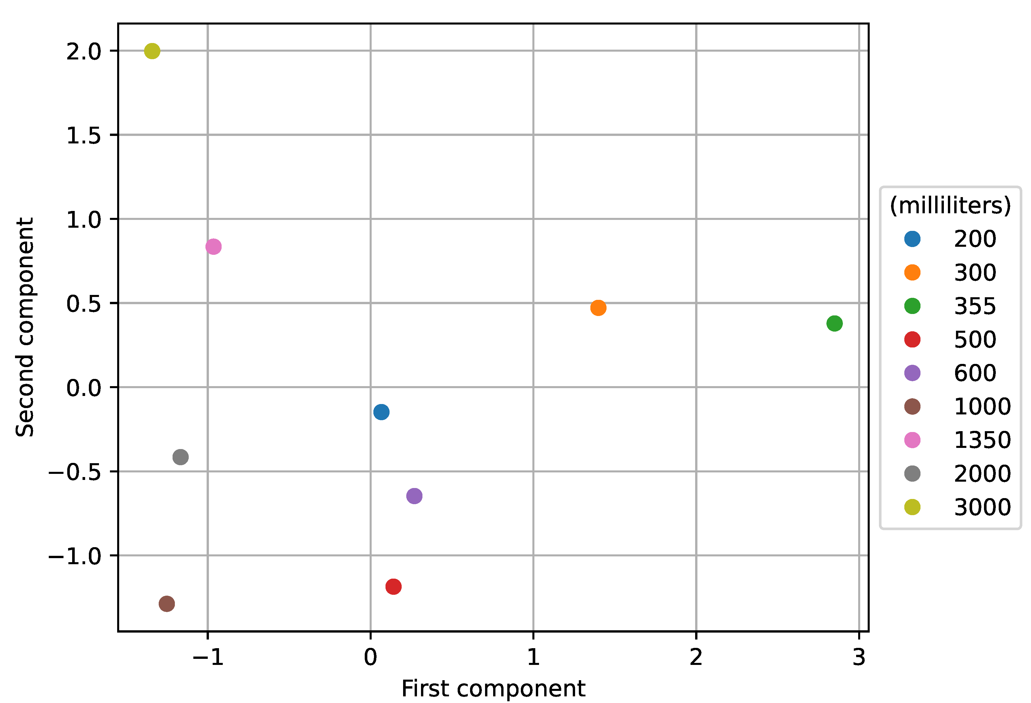
, the two principal components that represent 76.8% of the variation of the data the results are shown in the following Figure 12. he graph shows that the 3000 and 1350 bottles are the bottles that reflect the most illuminance, mainly due to their type of label. This behavior is due to its manufacturing design. The bottles 2000 and 1000 are bottles in which, when they have a label, their illuminance is high, and when they contain liquids, their illuminance is much lower than the other bottles. The 500 and 600 bottles have slight label variations but are more significant when the amount of liquids decreases. The 200 bottle is the most difficult to detect by its label and if it has liquids. The 300 and 355 bottles are bottles that are similar concerning its label when they have liquids inside the bottle. The 355 and 300 bottles with several liquids between 75 to 177 milliliters are the ones that have the most variation, with a distance of 25 cm concerning the conveyor belt.

In conclusion, the first component is the amount of variation the bottles have to detect liquids. The second component was interpreted as the variation that the bottles have with their label. With these results, it can be defined that at least two classes can be identified to determine the number of liquids inside the bottles.

3.4. Support Vector Machine

In Table 18, the bottles were classified with their different sizes and the number of liquids inside them.

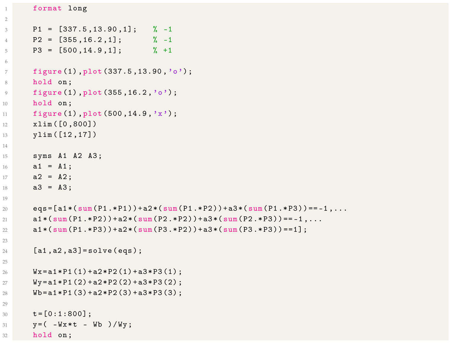
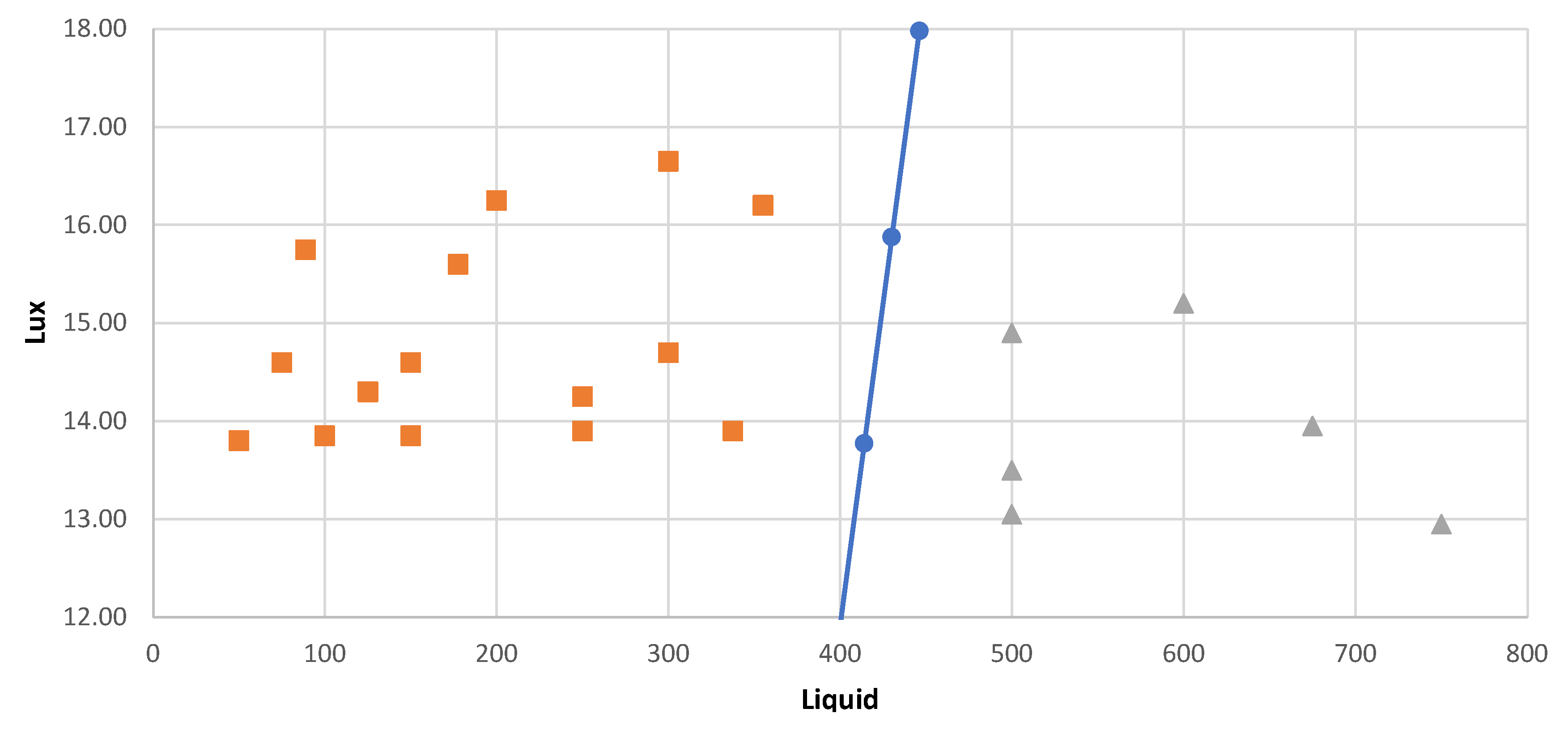
The development of SVM used a program in Matlab that can be consulted in Listing . Figure 13 shows that two classes were determined, one for bottles with liquids less than 337.5 milliliters and class two for bottles with more than 500 milliliters.

The SVM results help us determine the operating range to detect the number of liquids inside the bottle and the bottle size. As the number of classes increases in this analysis, the number of liquids inside the bottles could be determined better at an affordable cost of implementation.

3.5. Development of the Lux Meter and the Liquid Identification System

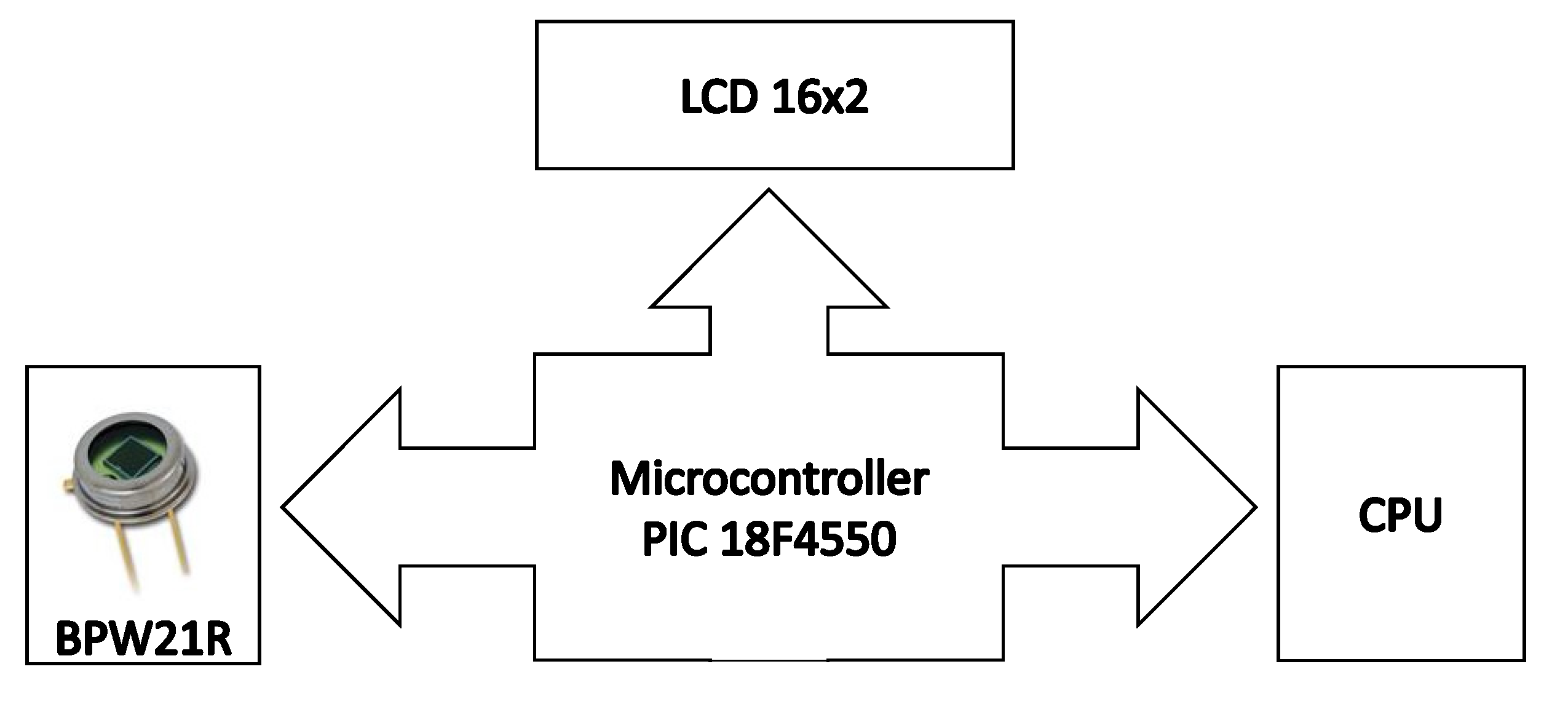
A system was developed that works in the visible spectrum. By measuring the luminous intensity, it is possible to identify if the liquid is inside the plastic bottle. At this stage, a lux meter was developed to be activated by identifying a bottle with no deformation; see Figure 14. Activation was done manually.

IR spectroscopy was used to detect the absorption of different light wavelengths in PET and labels. In the first stage of this configuration, work was done with an infrared photodiode that detects wavelengths in the range of 800 nm and 1100 nm, suitable for differentiating between transparent and colored PET and labels with different sizes and colors. A light source was installed to help the sensor better detect the type of plastic and to obtain the data. With the results of the three DOE and with statistical evidence, the working range was designed for optimal operating conditions and detection of wavelengths [28,29].

3.5.1. Functions to Estimate the Illuminance on the Sensor

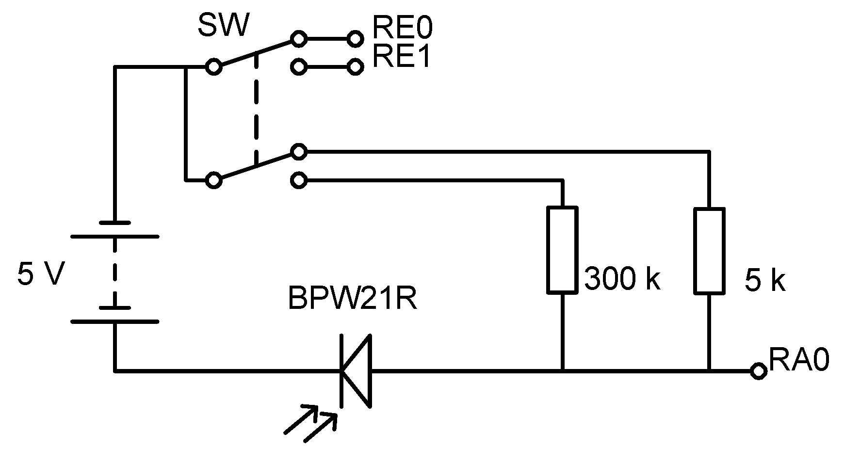
The value of the measurand was estimated, the law of Ohm was applied, see Equation (14), and 18 linear equations were calculated to obtain the electrical resistance in the entire working range of the photo-diode, see Figure 15.

The input signal to the microcontroller was not amplified because the readings were consistent. The variable resistance of the photodiode was estimated, and with it, the current of the circuit was calculated to assess the illuminance.

I = \frac{V}{R} = \frac{V o l t a g e}{R e s i s t a n c e_{v a r i a b l e} + R e s i s t a n c e_{f i x e d}}

(14)

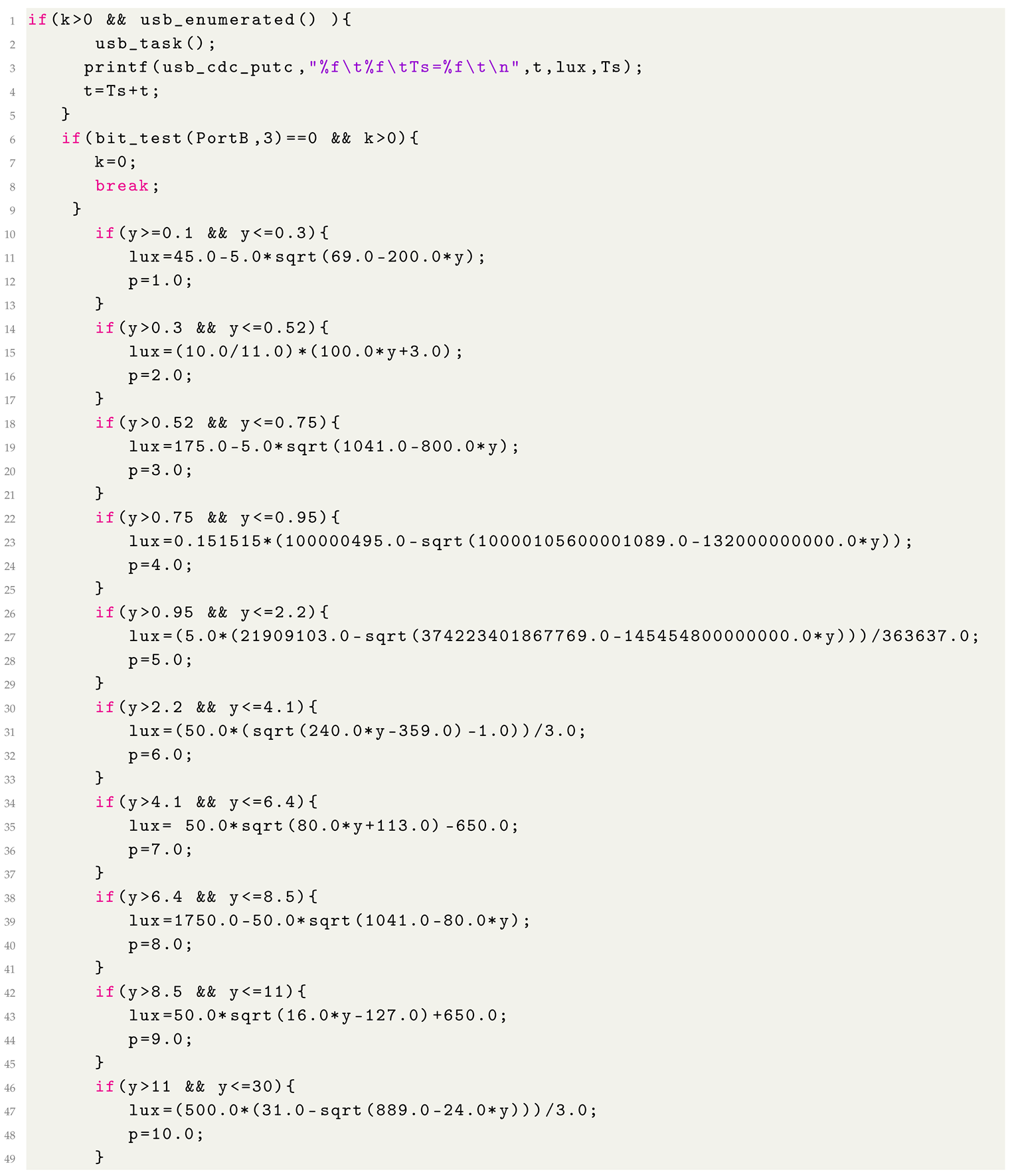
The first nine points of Table 19 were taken to obtain the equations that describe the photodiode, then interpolation of Newton was applied, and the variables were cleared.

Work intervals were estimated, and a function was determined using the current in the circuit. The results are the following: From 0 lux to less than 89 lux, we have the following Equations (15)-(17).

l u x = 45 - 5 \sqrt{69 - 200 I}

(15)

l u x = \frac{10}{11} (100 I + 3)

(16)

l u x = 175 - 5 \sqrt{1041 - 800 I}

(17)

Equation (18) from 90 to 200 lux

l u x = 0.151515 (100000495 - \sqrt{10000105600001089 - 132000000000 I})

(18)

Equation (19) from 200 to 400 lux

l u x = \frac{(5 (21909103 - \sqrt{374223401867769.0 - 145454800000000 I}))}{363637}

(19)

Equation (20) from 400 to 600 lux

l u x = \frac{(50 (\sqrt{240.0 I - 359.0} - 1.0))}{3}

(20)

Equation (21) from 600 to 800 lux

l u x = 50 \sqrt{80 I + 113} - 650

(21)

Equation (22) from 800 to 1000 lux

l u x = 1750 - 50 \sqrt{1041 - 80 I}

(22)

Equation (23) from 1000 to 3000 lux

l u x = 50 \sqrt{16 I - 127.0} + 650

(23)

Equation (24) from 3000 to 5000 lux

l u x = \frac{(500 (31 - \sqrt{889 - 24 I}))}{3}

(24)

Equation (25) from 5000 to 7000 lux

l u x = \frac{(1000 (I + 3))}{11}

(25)

Equation (26) from 7000 to 9000 lux

l u x = 17500 - 500 \sqrt{1041 - 8 I}

(26)

Equation (27) from 7000 to 20000 lux

l u x = 100 (I - 5)

(27)

Equation (28) from 20000 to 40000 lux

l u x = \frac{(500 (1825757 - \sqrt{2598770771809 - 10101000000 I}))}{30303}

(28)

Equation (29) from 40000 to 60000 lux

l u x = \frac{(1000 \sqrt{5} (\sqrt{12 I - 1795} - \sqrt{5}))}{3}

(29)

Equation (30) from 60000 to 80000 lux

l u x = 1000 \sqrt{5} \sqrt{4 I + 565} - 65000

(30)

Equation (31) from 80000 to 100000 lux

l u x = 175000 - 1000 \sqrt{5} \sqrt{5205 - 4 I}

(31)

Equation (32) greater than 100,000 lux

l u x = 1000 \sqrt{4 I - 3175} + 65000

(32)

3.5.2. Lux Meter

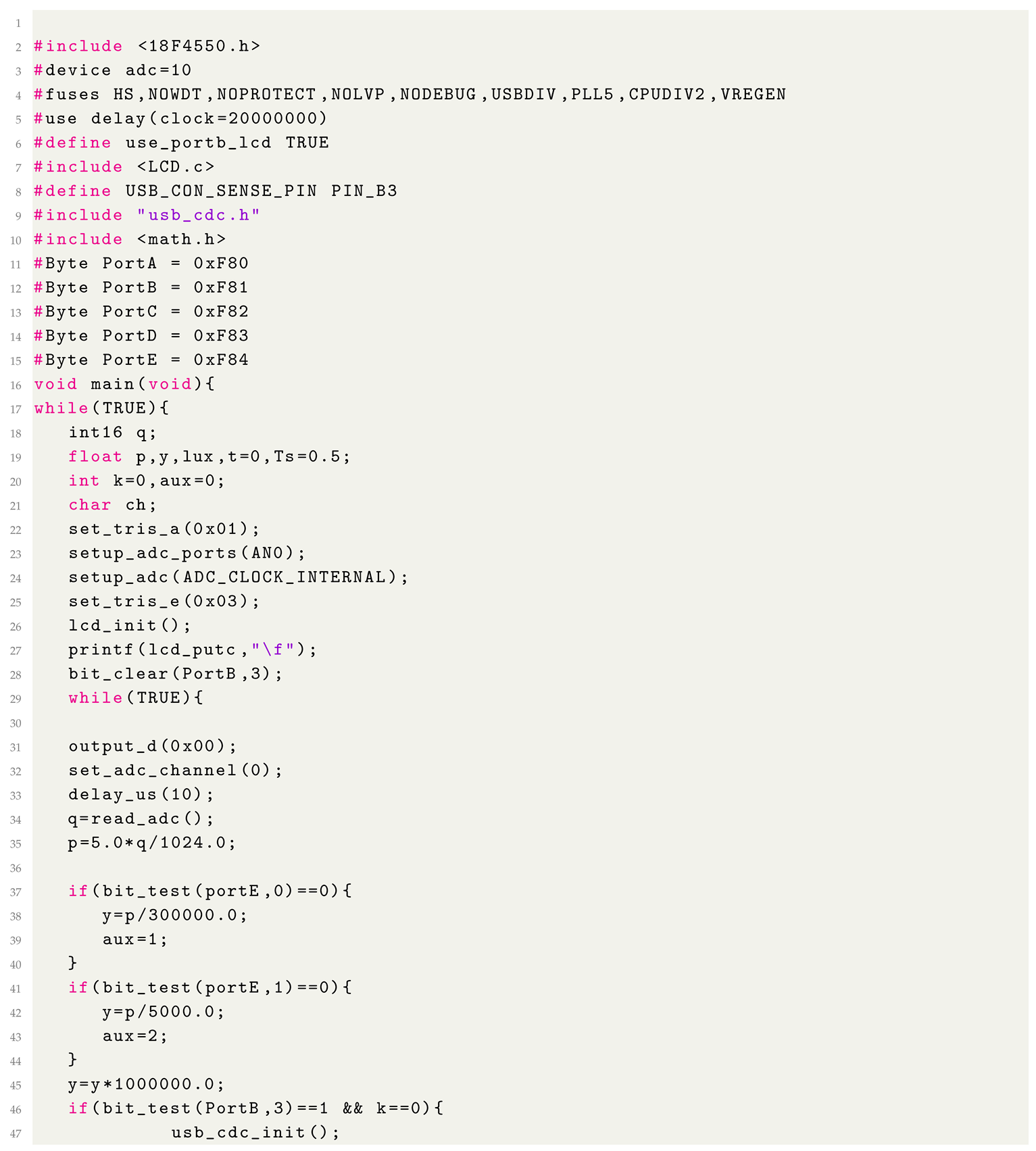
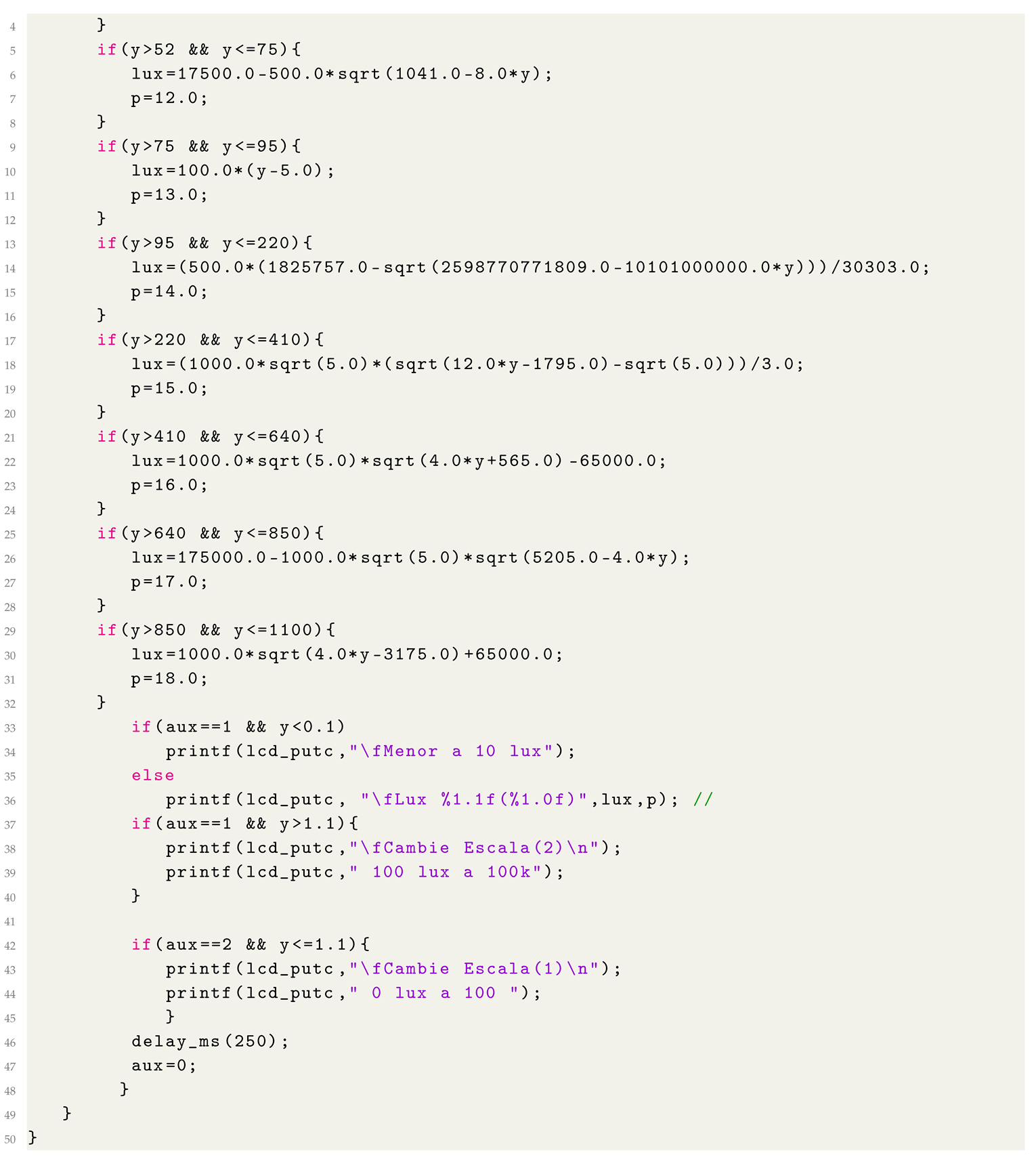
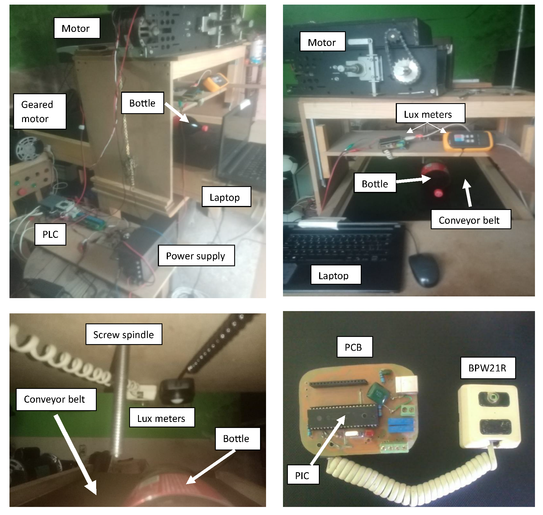
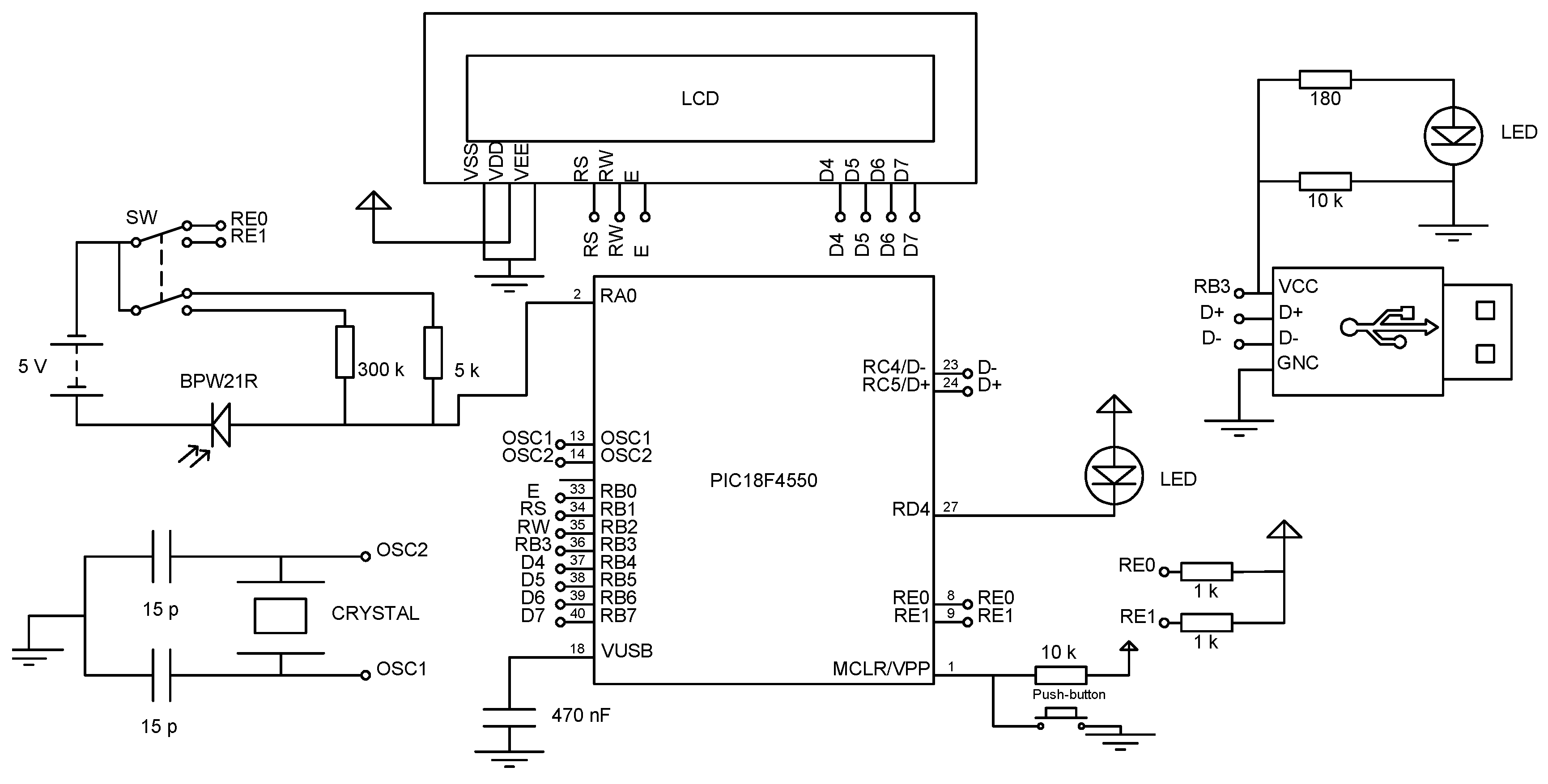
The above equations are programmed on a microcontroller and a PCB designed for implementation on the conveyor belt. The conveyor belt was designed so that the system would analyze three bottles per second. It can move forward and backward and be controlled by pulses through a PLC interface with a web page. The lux meter design can send the information through the USB port, and the data can be processed to identify liquids inside the bottles. Figure 16 shows the connections for the implementation and acquisition of the data.

Figure 17, shows the conveyor belt where the commercial lux meter and the proposed lux meter were installed. To detect the bottles, the conveyor belt starts and stops depending on the bottle when it passes entirely through the lux meter. The results coincide with the experimentation already mentioned above.

Listing to , shows the program used to program the digital lux meter. Figure A1 shows evidence of the lux meter design.

4. Discussion

With the results of the three experiments, the distance from the lux meter and the operating range in which the lux meter must work to identify if the bottles have liquids and thus approximate the number of liquids in a ton were obtained. The results of SVM showed that it is possible to approximate the amount of liquid a bottle may have. If the dimensions of the support vector machine are increased, it would be possible to optimize the system with the data. The results of this work are an effort to be implemented a video camera to identify the bottle size so that the lux meter can optimally approximate the amount of liquid. Another of the purposes of the work is to present in different papers the results of the development of an automated system to identify polymers for CC in Mexico. In the experimentation, it was only considered that the bottle would be in the direction of the conveyor belt. In other conditions, it has not been experimented with, so a camera that indicates the position of the bottle is a viable option to minimize the variation that the role of the bottle may have. Because this work is part of a larger one, the final result is not presented but part of the results to achieve better when combined with the vision system and the lux meter. In addition, to simplify the idea that we propose, we will implement at least three experimental designs to determine the factors that affect the processing of images in real-time in a test bed and to be able to generate premises for the design and development of an affordable classification system. from the academic field.

5. Conclusions

This work integrates classification technologies to demonstrate advances in the modern recycling of urban solid materials. It is necessary to emphasize that Mexico needs to develop techniques to increase the productivity of collection centers for recyclable materials and face the challenges that recycling implies.

It is possible to develop an automatic liquid identification system for recyclable polyethylene terephthalate bottles with an affordable design.
It was possible to develop a new methodology to be implemented to identify dark liquids.
It is possible to quantify the number of dark liquids that post-consumer PET bottles can have by implementing an affordable design.

This work has provided a solution for modernizing collection centers to increase the classification of post-consumer PET bottles.

Author Contributions

Conceptualization, L.A.-A, and J.R.-R; methodology, L.A.-A; software, L.A.-A; validation, J.R.-G, H.R.-Z, H.T.-Z, and J.R.-R; formal analysis, L.A.-A; investigation, L.A.-A; resources, L.A.-A and J.R-R; data curation, L.A.-A; writing—original draft preparation, J.R-R, J.R.-G, H.T.-S, and H.R.-Z; writing—review and editing, J.R.-G, J.R-R, H.T.-S, S.P.-S and H.R.-Z; visualization, L.A.-A; supervision, H.R.-Z, and J.R-R; project administration, L.A.-A; funding acquisition, J.R.-G, L.A.-A, J.R.-R, and S.P.-S All authors have read and agreed to the published version of the manuscript.

Funding

CONAHCYT funded this research.

Institutional Review Board Statement

Not applicable.

Informed Consent Statement

Not applicable.

Acknowledgments

This work was carried out thanks to the support of the Autonomous University of Querétaro and Materiales Reciclables Ángeles, Querétaro.

Conflicts of Interest

The authors declare no conflict of interest. The funders had no role in the study’s design; in the collection, analyses, or interpretation of data; in the writing of the manuscript, or in the decision to publish the results.

Abbreviations

The following abbreviations are used in this manuscript:

ANOVA	analysis of variance
CC	Collection Centers
DIL40	40 PINS Dual-in-line package
DOE	Design of Experiments
F	F Ratio
gl	Degrees of Freedom
LCD	Liquid-crystal display
LED	light-emitting diode
MS	Mean Squarese
ml	Milliliters
NC	Normally closed
No.	number
PC1	First principal component
PC2	Second principal component
PCA	Principal component analysis
PCB	Printed circuit board
PET	Polyethylene Terephthalate
PIC	Peripheral Interface Controller
SVM	Support vector machine
SS	Sum of squares
USE	Universal Serial Bus

Appendix A

Listing 1: Code for the SVM algorithm in Matlab.

Appendix B

Listing 2: Code for programming the lux meter in c.

Listing 3: Code for programming the lux meter in c.

Listing 4: Code for programming the lux meter in c.

Appendix C

Figure A1. Photos of the experiment workbench.

References

OECD. Plastic pollution is growing relentlessly as waste management and recycling fall short, 2022.
La Mantia, F.P.; Scaffaro, R.; Baiamonte, M.; Ceraulo, M.; Mistretta, M.C. Comparison of the Recycling Behavior of a Polypropylene Sample Aged in Air and in Marine Water. Polymers 2023, 15. [CrossRef]
Ángeles-Hurtado, L.A.; Rodríguez-Reséndiz, J.; Salazar-Colores, S.; Torres-Salinas, H.; Sevilla-Camacho4, P.Y. Viable Disposal of Post-Consumer Polymers in Mexico: A Review. Frontiers in Environmental Science 2021, 9, 427. [CrossRef]
cuentame.inegi.org.mx. Medio ambiente - Basura; Fecha de la consulta 06/05/2020, 2020.
Hernández Huerta, A. Caja de herramientas para la formación ambiental; Vol. 1, Instituto de Ecología, A.C, 2018.
Hejna, A. Renewable, Degradable, and Recyclable Polymer Composites. Polymers 2023, 15. [CrossRef]
de Coca-Cola (IMCC), I.M. Entérate qué es la Industria Mexicana de Coca-Cola y quiénes formamos parte de ella 27/05/2019, 2019.
Christakopoulos, F.; van Heugten, P.M.H.; Tervoort, T.A. Additive Manufacturing of Polyolefins. Polymers 2022, 14. [CrossRef]
Peláez Lenis, L.C.; Olmos Rodríguez, M.C.; others. Plan de empresa para la creación de Recoplast, empresa dedicada a la recuperación de plásticos reciclables. B.S. thesis, Universidad Autónoma de Occidente, 2018.
Garraín, D.; Vidal, R.; Franco, V.; Martínez, P. Análisis del ciclo de vida del reciclado del polietileno de alta densidad. Residuos 2008, 104, 58–63.
Ramli, S.; Mustafa, M.M.; Hussain, A.; Wahab, D.A. Histogram of intensity feature extraction for automatic plastic bottle recycling system using machine vision. American Journal of Environmental Sciences 2008, 4, 583.
Lundell, C.; Thomas, J. PET: Polyethylene Terephthalate – The Ubiquitous 500 ml Water Bottle; Vol. 1202 AISC, Advances in Intelligent Systems and Computing, scopus, 2020; pp. 248–254.
Al-Salem, S.M.; Lettieri, P.; Baeyens, J. Recycling and recovery routes of plastic solid waste (PSW): A review. Waste Management 2009, 29, 2625–2643. Cited By :1018.
Sahin, O.; Kirim, Y., Material Recycling. In Comprehensive Energy Systems; scopus, 2018; Vol. 2-5, Comprehensive Energy Systems, pp. 1018–1042. Cited By :2.
Chu, J.; Hu, X.; Kong, L.; Wang, N.; Zhang, S.; He, M.; Ouyang, W.; Liu, X.; Lin, C. Dynamic flow and pollution of antimony from polyethylene terephthalate (PET) fibers in China. Science of the Total Environment 2021, 771. Cited By :2.
Ardusso, M.; Forero-López, A.D.; Buzzi, N.S.; Spetter, C.V.; Fernández-Severini, M.D. COVID-19 pandemic repercussions on plastic and antiviral polymeric textile causing pollution on beaches and coasts of South America. Science of the Total Environment 2021, 763. Cited By :2.
Guo, H.; Mettas, A. Design of experiments and data analysis. 2012 Annual Reliability and Maintainability Symposium, 2010.
Gutiérrez Pulido, H.; Vara Salazar, R.d.l. Análisis y diseño de experimentos; McGrawHill, 2004.
Escalante Vázquez, E.J. Seis-Sigma Metodología y técnicas; Editorial Limusa: México: Limusa, 2007, 2007.
Kumar, P.A. Classification of Power Quality Events Using Support Vectir Machine and S-Transform. 2016 2nd International Conference on Contemporary Computing and Informatic 2003, 7, 279–284.
Rizanti, Nova Ayu AriniSetianingrum, A.H. Colon detection using Principal Component Analysis (PCA) and Support Vector Machine (SVM). IEEE 2016, pp. 1–6.
Ashwini S. Shinde, S.S.J.; Puranik, V. Identification and Sorting of Power Quality Disturbances Using Signal Processing with GUI. E International Conference on Advances in Electronics, Communication and Computer Technology (ICAECCT) Rajarshi Shahu College of Engineering, Pune India. 2016, pp. 60–63.
Vapnik, V.N. An overview of statistical learning theory. IEEE Transactions on Neural Networks 1999, 10, 988–999.
Kumar, Pradeep Krishna, P.R.L.; Infosys Raju, S.B. Pattern Discovery Using Sequence Data Mining; Information Science Reference, 2011.
Rani, M.; Marchesi, C.; Federici, S.; Rovelli, G.; Alessandri, I.; Vassalini, I.; Ducoli, S.; Borgese, L.; Zacco, A.; Bilo, F.; Bontempi, E.; Depero, L. Miniaturized near-infrared (MicroNIR) spectrometer in plastic waste sorting. Materials 2019, 12. cited By 1. [CrossRef]
Semiconductors, V. Silicon PN Photodiode. Technical report, Vishay Semiconductor GmbH, P.O.B. 3535, D-74025 Heilbronn, Germany, 2006.
Semiconductors, V. Measurement Techniques: Document Number: 80085. Technical report, Vishay Semiconductor GmbH, P.O.B. 3535, D-74025 Heilbronn, Germany, 2008.
T Huth-Fehre, R Feldhoff, T.K.; Quick., L. NIR - Remote Sensing and Artificial Neural Networks for Rapid Identification of Post Consumer Plastics. Journal of Molecular Structure 1995.
S.M., S.; H., M.; S.S., M.; Tabrizchi, M. Sorting of polypropylene resins by color in MSW using visible reflectance spectroscopy. Waste Management 2010, 30, 2216–2222. cited By 23. [CrossRef]

Figure 1. Diagram of the new methodology for designing and developing the liquid identification system.

Figure 2. Different presentations of PET bottles in the Mexican market.

Figure 3. Flowchart of the manual sorting process for PET bottles.

Figure 4. Factors and variables of the first design of experiments.

Figure 5. Discrimination system through the detection of liquids in PET bottles by their illuminance.

Figure 6. Factors and variables in the second design of experiments.

Figure 7. Detection system for liquids in PET bottles due to their illuminance.

Figure 8. Response graph with the interaction of factors A and B.

Figure 9. Discrimination system through liquid detection.

Figure 10. Response graph with the interaction of the second experiment.

Figure 11. Response plot of the third experiment.

Figure 12. The plot of scores for the two principal components.

Figure 13. SVM graph to identify the number of liquids in PET bottles.

Figure 14. Block diagram of the lux meter data acquisition system.

Figure 15. Sensor data reading system circuit.

Figure 16. Circuit diagram and data acquisition.

Figure 17. Conveyor belt.

Table 1. Type of material and amount separated in 2018 [4].

Material Type	Percentage
Other plastics	42
Iron, and steel	29
Paper and carton	17
PET	6
Other materials	5
Glass	1

Table 2. Conveyor belt design parameters.

No.	Name	Parameter	Expression	Value
1	Band base width	bandBaseWidth	90 cm	90.0
2	Long band base	LongBandBase	200 cm	200.0
3	Band leg base	BandLegBase	10 cm	10.0
4	Table base width	TableBaseWidth	bandBaseWidth + (BandLegBase*4)	130.0
5	Long table base	LongTableBase	70 cm	70.0
6	High table base	HighTableBase	2 cm	2.0
7	Wide leg base	WideLegBase	70 mm	70.0
8	Long leg base	LongLegBase	150 mm	150.0
9	High leg base	HighLegBase	10 mm	10.0
10	Wide leg	WideLeg	35 mm	35.0
11	Long leg	LongLeg	100 mm	100.0
12	High leg	HighLeg	70 cm	70.0
13	Table plan	TablePlan	HighLeg + HighLegBase	101.0
14	Bottom box width	BottomBoxWidth	TableBaseWidth - 10 cm	120.0
15	Long box base	LongBoxBase	LongTableBase - 2 cm	68.0
16	Base box thickness	BaseBoxThickness	2 cm	2.0
17	High box base	HighBoxBase	60 cm	60.0
18	Height tab	HeightTab	HighBoxBase / 1.5	40.0
19	Base Rail Width	BaseRailWidth	4.5 cm	4.5
20	Base Long Rail	BaseLongRail	30 cm	30.0
21	Base Rail Thickness	BaseRailThickness	1.3 cm	1.3
22	Base Chamber Width	BaseChamberWidth	TableBaseWidth - 20 cm	110.0
23	Base Chamber Length	BaseChamberLength	LongTableBase - 10 cm	60.0

Table 3. The material used for the PCB of the lux meter.

No.	Material	Type	Volume
1	LCD	16X2	1
2	MICROCONTROLLER	18F4550	1
3	SENSOR	bpw21r	1
4	CONNECTOR	MOLEX	3
5	POTENTIOMETER	1M	1
6	POTENTIOMETER	5k	1
7	RESISTOR	1K	6
8	RESISTOR	10K	8
9	RESISTOR	220	4
10	CAPACITOR	470n	3
11	CAPACITOR	15p	4
12	CAPACITOR	0.1u	2
13	CAPACITOR	1u	2
14	CAPACITOR	0.33u	2
15	LED	RED	3
16	CRYSTAL	20M	1
17	DIL40	40 PINS	1
18	PINS	MALE	1
19	PINS	FEMALE	1
20	PHENOLIC BOARD	COPPER	1
21	ACID	FeCl3	1
22	USB CONNECTOR	B	1
23	TEL CONNECTOR	4 HILOS	1
24	SWICH 1	POLO 2	2
25	HOUSING	BLACK	1
26	BUTTON	NC	1

Table 4. General guidelines for conducting DOE.

Objective DOE 1	Identify important factors from many potential factors
Response	Iluminancia
Factor and Levels	Distance and three levels
Factor and Levels	Bottle size and nine levels
Objective DOE 2	Identify important factors from many potential factors
Response	Illuminance
Factor and Levels	Percentage of liquids inside the bottle and three levels
Factor and Levels	Bottle size and nine levels
Objective DOE 3	Identify important factor
Response	Illuminance
Factor and Levels	Types of labels on bottles

Table 5. Approach to the design of experiments for the position of the lux meter considering two factors.

		Lux meter distance (A)
		15	20	25	Sum
Bottle Size (B)	200 ml	$y_{i j}$	$y_{i j}$	$y_{i j}$
		$y_{i j}$	$y_{i j}$	$y_{i j}$	$S u m_{j}$
	Sum	$S u m_{i j}$	$S u m_{i j}$	$S u m_{i j}$
	300 ml	$y_{i j}$	$y_{i j}$	$y_{i j}$
		$y_{i j}$	$y_{i j}$	$y_{i j}$	$S u m_{j}$
	Sum	$S u m_{i j}$	$S u m_{i j}$	$S u m_{i j}$
	355 ml	$y_{i j}$	$y_{i j}$	$y_{i j}$
		$y_{i j}$	$y_{i j}$	$y_{i j}$	$S u m_{j}$
	Sum	$S u m_{i j}$	$S u m_{i j}$	$S u m_{i j}$
	500 ml	$y_{i j}$	$y_{i j}$	$y_{i j}$
		$y_{i j}$	$y_{i j}$	$y_{i j}$	$S u m_{j}$
	Sum	$S u m_{i j}$	$S u m_{i j}$	$S u m_{i j}$
	600 ml	$y_{i j}$	$y_{i j}$	$y_{i j}$
		$y_{i j}$	$y_{i j}$	$y_{i j}$	$S u m_{j}$
	Sum	$S u m_{i j}$	$S u m_{i j}$	$S u m_{i j}$
	1000 ml	$y_{i j}$	$y_{i j}$	$y_{i j}$
		$y_{i j}$	$y_{i j}$	$y_{i j}$	$S u m_{j}$
	Sum	$S u m_{i j}$	$S u m_{i j}$	$S u m_{i j}$
	1350 ml	$y_{i j}$	$y_{i j}$	$y_{i j}$
		$y_{i j}$	$y_{i j}$	$y_{i j}$	$S u m_{j}$
	Sum	$S u m_{i j}$	$S u m_{i j}$	$S u m_{i j}$
	2000 ml	$y_{i j}$	$y_{i j}$	$y_{i j}$
		$y_{i j}$	$y_{i j}$	$y_{i j}$	$S u m_{j}$
	Sum	$S u m_{i j}$	$S u m_{i j}$	$S u m_{i j}$
	3000 ml	$y_{i j}$	$y_{i j}$	$y_{i j}$
		$y_{i j}$	$y_{i j}$	$y_{i j}$	$S u m_{j}$
	Sum	$S u m_{i j}$	$S u m_{i j}$	$S u m_{i j}$
	Sum Total	$S u m T_{i}$	$S u m T_{i}$	$S u m T_{i}$	$S u m T$

Table 6. Summary of the first two-way ANOVA.

Source	SS	gl	MS	F
Distance (A)	SSA	a-1	MSA = SSA/(a-1)	MSA / MSE
Bottle (B)	SSB	b-1	MSB = SSB/(b-1)	MSB / MSE
AB	SSAB	a-1	MSAB = SSAB/(a-1)	MSAB / MSE
Error	SSE	N-a-b-1	MSE = SSE/(N-a-b-1)
Total	SST	N-1

Table 7. Approach to the design of experiments to identify the percentage of liquid in the bottles.

		Percentage of liquid in the bottle (A)
		50 %	25 %	0 %	Sum
Bottle Size (B)	200 ml	$y_{i j}$	$y_{i j}$	$y_{i j}$
		$y_{i j}$	$y_{i j}$	$y_{i j}$	$S u m_{j}$
	Sum	$S u m_{i j}$	$S u m_{i j}$	$S u m_{i j}$
	300 ml	$y_{i j}$	$y_{i j}$	$y_{i j}$
		$y_{i j}$	$y_{i j}$	$y_{i j}$	$S u m_{j}$
	Sum	$S u m_{i j}$	$S u m_{i j}$	$S u m_{i j}$
	355 ml	$y_{i j}$	$y_{i j}$	$y_{i j}$
		$y_{i j}$	$y_{i j}$	$y_{i j}$	$S u m_{j}$
	Sum	$S u m_{i j}$	$S u m_{i j}$	$S u m_{i j}$
	500 ml	$y_{i j}$	$y_{i j}$	$y_{i j}$
		$y_{i j}$	$y_{i j}$	$y_{i j}$	$S u m_{j}$
	Sum	$S u m_{i j}$	$S u m_{i j}$	$S u m_{i j}$
	600 ml	$y_{i j}$	$y_{i j}$	$y_{i j}$
		$y_{i j}$	$y_{i j}$	$y_{i j}$	$S u m_{j}$
	Sum	$S u m_{i j}$	$S u m_{i j}$	$S u m_{i j}$
	1000 ml	$y_{i j}$	$y_{i j}$	$y_{i j}$
		$y_{i j}$	$y_{i j}$	$y_{i j}$	$S u m_{j}$
	Sum	$S u m_{i j}$	$S u m_{i j}$	$S u m_{i j}$
	1350 ml	$y_{i j}$	$y_{i j}$	$y_{i j}$
		$y_{i j}$	$y_{i j}$	$y_{i j}$	$S u m_{j}$
	Sum	$S u m_{i j}$	$S u m_{i j}$	$S u m_{i j}$
	2000 ml	$y_{i j}$	$y_{i j}$	$y_{i j}$
		$y_{i j}$	$y_{i j}$	$y_{i j}$	$S u m_{j}$
	Sum	$S u m_{i j}$	$S u m_{i j}$	$S u m_{i j}$
	3000 ml	$y_{i j}$	$y_{i j}$	$y_{i j}$
		$y_{i j}$	$y_{i j}$	$y_{i j}$	$S u m_{j}$
	Sum	$S u m_{i j}$	$S u m_{i j}$	$S u m_{i j}$
	Sum Total	$S u m T_{i}$	$S u m T_{i}$	$S u m T_{i}$	$S u m T$

Table 8. Approach to the design of experiments to identify the variability with the labels.

			Replicas
		1	2	3	4	5	6	Sum	y	$s^{2}$
Bottle Size (A)	3000 ml	$y_{i j}$	$y_{i j}$	$y_{i j}$	$y_{i j}$	$y_{i j}$	$y_{i j}$	$S u m_{j}$	$y_{j}$	$s_{j}^{2}$
	2000 ml	$y_{i j}$	$y_{i j}$	$y_{i j}$	$y_{i j}$	$y_{i j}$	$y_{i j}$	$S u m_{j}$	$y_{j}$	$s_{j}^{2}$
	1350 ml	$y_{i j}$	$y_{i j}$	$y_{i j}$	$y_{i j}$	$y_{i j}$	$y_{i j}$	$S u m_{j}$	$y_{j}$	$s_{j}^{2}$
	1000 ml	$y_{i j}$	$y_{i j}$	$y_{i j}$	$y_{i j}$	$y_{i j}$	$y_{i j}$	$S u m_{j}$	$y_{j}$	$s_{j}^{2}$
	600 ml	$y_{i j}$	$y_{i j}$	$y_{i j}$	$y_{i j}$	$y_{i j}$	$y_{i j}$	$S u m_{j}$	$y_{j}$	$s_{j}^{2}$
	500 ml	$y_{i j}$	$y_{i j}$	$y_{i j}$	$y_{i j}$	$y_{i j}$	$y_{i j}$	$S u m_{j}$	$y_{j}$	$s_{j}^{2}$
	355 ml	$y_{i j}$	$y_{i j}$	$y_{i j}$	$y_{i j}$	$y_{i j}$	$y_{i j}$	$S u m_{j}$	$y_{j}$	$s_{j}^{2}$
	300 ml	$y_{i j}$	$y_{i j}$	$y_{i j}$	$y_{i j}$	$y_{i j}$	$y_{i j}$	$S u m_{j}$	$y_{j}$	$s_{j}^{2}$
	250 ml	$y_{i j}$	$y_{i j}$	$y_{i j}$	$y_{i j}$	$y_{i j}$	$y_{i j}$	$S u m_{j}$	$y_{j}$	$s_{j}^{2}$
	200 ml	$y_{i j}$	$y_{i j}$	$y_{i j}$	$y_{i j}$	$y_{i j}$	$y_{i j}$	$S u m_{j}$	$y_{j}$	$s_{j}^{2}$

Table 9. Summary of the third ANOVA with one factor.

Source of variation	SS	gl	MS	F
Treatments (t)	SSt	a-1	MSt = SSt/(a-1)	MSt / MSE
Error	SSE	N-a	MSE = SSE/(N-a)
Total	SST	N-1

Table 10. Results of a 100 kg sample of post-consumer PET.

Bottles that were repeated the most.
No.	Bottle	Frequency	%	Accumulated
1	0.6 L	1307	26.356	26.356
2	1.0 L	837	16.878	43.234
3	1.5 L	653	13.167	56.402
4	2.0 L	642	12.946	69.348
5	3.0 L	382	7.703	77.051
6	0.5 L	346	6.977	84.029
7	0.35 L	294	5.928	89.957
8	0.25 L	205	4.133	94.091

Table 11. Information from the first ANOVA of two factors.

		Lux Meter distance (A)
		15	20	25	Sum
Bottle Size (B)	200 ml	13.4	14.9	16.5
		12.7	14.5	16	88
	Sum	26.1	29.4	32.5
	300 ml	12.4	14.4	16.7
		13.1	12.7	16.6	85.9
	Sum	25.5	27.1	33.3
	355 ml	13	15.2	16.2
		13.9	14.9	16.2	89.4
	Sum	26.9	30.1	32.4
	500 ml	13.6	13.9	14.8
		13.3	13.6	15	84.2
	Sum	26.9	27.5	29.8
	600 ml	12.5	13.9	15
		13.1	12.7	15.4	82.6
	Sum	25.6	26.6	30.4
	1000 ml	13.9	14	15.1
		13.1	14.7	15	85.8
	Sum	27	28.7	30.1
	1350 ml	15.6	15.2	16.4
		13.4	16.5	15.5	92.6
	Sum	29	31.7	31.9
	2000 ml	10.7	16.8	14.3
		9	17.5	14.9	83.2
	Sum	19.7	34.3	29.2
	3000 ml	5.2	19.3	17
		3.9	18.5	16	79.9
	Sum	9.1	37.8	33
	Sum Total	215.8	273.2	282.6	771.6

Table 12. ANOVA of the first experiment.

Source	SS	gl	MS	F
Distance (A)	145.2844	2	72.6422	259.8892*
Bottle (B)	19.73	8	2.4662	8.8234*
AB	194.5788	2	97.2894	348.0686*
Error	11.46	41	0.2795
Total	371.0533	53

Table 13. Information from the second two-way ANOVA.

		% Liquid in the bottle (A)
		50	25	0	Sum
Bottle Size (B)	200 ml	13.3	14.3	15
		14.4	13.3	15.2	85.5
	Sum	27.7	27.6	30.2
	300 ml	14.7	14.8	15
		14.5	14.4	15.3	88.7
	Sum	29.2	29.2	30.3
	355 ml	16.5	16.3	15.5
		14.7	15.2	16	94.2
	Sum	31.2	31.5	31.5
	500 ml	14.5	14.5	14.5
		14	14.1	15.4	87
	Sum	28.5	28.6	29.9
	600 ml	15.1	14	14
		14.3	13.7	15	86.1
	Sum	29.4	27.7	29
	1000 ml	12.2	14.2	13.5
		13.9	13.6	15.2	82.6
	Sum	26.1	27.8	28.7
	1350 ml	14.5	14.4	13.4
		13.4	13.4	15	84.1
	Sum	27.9	27.8	28.4
	2000 ml	15.1	13.7	13.4
		13.8	13.3	16	85.3
	Sum	28.9	27	29.4
	3000 ml	15.2	13.2	12.2
		13.7	12.7	15.3	82.3
	Sum	28.9	25.9	27.5
	Sum Total	257.8	253.1	264.9	775.8

Table 14. Results of the ANOVA of the second experiment.

Source	SS	gl	MS	F
% Liquid (A)	3.921	2	1.9605	3.8442*
Bottle (B)	17.4633	8	2.1829	4.2802*
AB	5.7855	2	2.8927	5.6721*
Error	20.91	41	0.51
Total	48.08	53

Table 15. Results design of experiments to identify the variability with the labels.

			Replicas
		1	2	3	4	5	6	Sum	y	$s^{2}$
Bottle Size (A)	3000 ml	30.00	28.10	25.20	24.10	26.00	29.80	163.20	27.20	6.092
	2000 ml	26.5	26.4	24.5	23.4	22.1	21.6	144.5	24.08	4.38
	1350 ml	22	26.7	25.7	25.8	27	28.4	155.6	25.93	4.67
	1000 ml	20.8	21.1	21.3	20.3	19.8	19.4	122.7	20.45	0.563
	600 ml	18.2	18.4	18.2	18.5	18.3	18.3	109.9	18.32	0.013
	500 ml	18.2	18.5	18.9	19.1	19	18.8	112.5	18.75	0.115
	355 ml	18.4	18.5	18.5	19.1	18.3	18	110.8	18.47	0.13
	300 ml	18	17.5	17.8	17.5	18.2	17.9	106.9	17.82	0.07
	250 ml	17.9	18.1	17.9	18.4	18.5	17.9	108.7	18.12	0.073
	200 ml	16.6	17.8	17.3	17.8	17.9	18	105.4	17.57	0.282

Table 16. One-way ANOVA of the third experiment.

Source of variation	SS	gl	MS	F
Treatments (t)	722.48	9	80.27	48.92*
Error	82.04	50	1.64
Total	804.52	59

Table 17. Data and results of the PCA.

		100% Liquid	50% Liquid	25% Liquid	Label	PC1	PC2
Bottle Size	3000 ml	16.50	14.45	12.95	27.20	-1.34137	1.99768
	2000 ml	14.60	14.45	13.50	24.08	-1.16713	-0.41555
	1350 ml	15.95	13.95	13.90	25.93	-0.96440	0.83528
	1000 ml	15.05	13.05	13.90	20.45	-1.25152	-1.28753
	600 ml	15.20	14.70	13.85	18.32	0.26894	-0.64694
	500 ml	14.90	14.25	14.30	18.75	0.14066	-1.18554
	355 ml	16.20	15.60	15.75	18.47	2.84955	0.37889
	300 ml	16.65	14.60	14.60	17.82	1.39885	0.47160
	200 ml	16.25	13.85	13.80	17.57	0.06642	-0.14789

Table 18. Classes for parsing SVM.

	Class	1		Class	2
% Liquid	Liquid	Illuminance	% Liquid	Liquid	Illuminance
100%	355	16.20	100%	1000	15.05
100%	300	16.65	100%	600	15.2
100%	200	16.25	100%	500	14.9
50%	177.5	15.60	50%	500	13.05
50%	150	14.60	100%	3000	16.50
50%	100	13.85	100%	2000	14.60
25%	88.75	15.75	100%	1350	15.95
25%	75	14.60	50%	1500	14.45
25%	50	13.80	50%	1000	14.45
50%	300	14.7	50%	675	13.95
50%	250	14.25	25%	750	12.95
25%	250	13.9	25%	500	13.50
25%	150	13.85
25%	125	14.3
25%	337.5	13.9

Table 19. Data to obtain the equations of the operation of the photodiode.

No.	EA-Iluminancia (lx)	lK-Short-circuit current (mA)
1	0.01	0.0001
2	0.1	0.00086
3	1	0.0092696
4	10	0.09172
5	100	0.967639
6	1000	9.712874
7	10000	96.64246
8	100000	972.178
9	912669	1000

Disclaimer/Publisher’s Note: The statements, opinions and data contained in all publications are solely those of the individual author(s) and contributor(s) and not of MDPI and/or the editor(s). MDPI and/or the editor(s) disclaim responsibility for any injury to people or property resulting from any ideas, methods, instructions or products referred to in the content.

© 2023 by the authors. Licensee MDPI, Basel, Switzerland. This article is an open access article distributed under the terms and conditions of the Creative Commons Attribution (CC BY) license (http://creativecommons.org/licenses/by/4.0/).

Copyright: This open access article is published under a Creative Commons CC BY 4.0 license, which permit the free download, distribution, and reuse, provided that the author and preprint are cited in any reuse.

MDPI Initiatives

Important Links

Choose an area of interest and we will send you notifications of new preprints at your preferred frequency.

Disclaimer

Development of a Lux Meter for the Identification of Liquids in Post-Consumer Polyethylene Terephthalate Bottles for Collection Centers in Mexico

Abstract

1. Introduction

2. Methodology

2.1. Post-Consumer PET Bottles

2.1.1. Physical Characteristics of Post-Consumer PET Bottles

2.1.2. Reducing the Problem to an Empirical Level

2.2. Materials

2.2.1. Mechanical Design Parameters

2.2.2. Electronic Card

2.3. Description of the Manual Bottle Classification Process

2.4. Design of Experiments for Variable Identification

2.4.1. Design of Experiments to Determine the Distance and Working Range of the Lux Meter

2.4.2. Design of Experiments to Identify the Minimum Amount of Liquids Inside the Bottle

2.4.3. Design of Experiments to Determine Label Illuminance

2.5. Principal Component Analysis

2.6. Support Vector Machine

2.7. Development of the Lux Meter and Liquid Identification System

2.7.1. Definition of the Measurand for the Measurement of Illuminance

2.7.2. Ambient Light Sensor BPW21R

3. Results

3.1. Sample Results of the Classification Process Manually

3.2. Design of Experiments for Variable Identification

3.2.1. Design of Experiments to Determine the Distance and Working Range of the Lux Meter

3.2.2. Design of Experiments to Identify the Minimum Amount of Liquids Inside the Bottle

3.2.3. Design of Experiments to Determine the Illuminance on the Labels

3.3. Principal Component Analysis, PCA

3.4. Support Vector Machine

3.5. Development of the Lux Meter and the Liquid Identification System

3.5.1. Functions to Estimate the Illuminance on the Sensor

3.5.2. Lux Meter

4. Discussion

5. Conclusions

Author Contributions

Funding

Institutional Review Board Statement

Informed Consent Statement

Acknowledgments

Conflicts of Interest

Abbreviations

Appendix A

Appendix B

Appendix C

References

MDPI Initiatives

Important Links

Subscribe