Investigation of Following Vehicle Driving Pattern using Spectral Analysis Techniques

Preprint

Article

Investigation of Following Vehicle Driving Pattern using Spectral Analysis Techniques

Altmetrics

Downloads

Views

Comments

A peer-reviewed article of this preprint also exists.

This version is not peer-reviewed

Submitted:

02 June 2023

Posted:

02 June 2023

You are already at the latest version

Alerts

Abstract

The key to ensuring the sustainability of transportation operations on the roads is to manage traffic flows homogeneously. By homogenizing the behavior of various drivers, traffic operation can be optimized, and traffic safety can be improved. However, the advent of autonomous vehicles is expected to have a major impact on the homogeneity of sustainable transportation operations. In this study, a method of driving in harmony with surrounding vehicles was studied to minimize the impact of autonomous vehicles on current traffic operation. In particular, in this study, a methodology was developed to optimize the driving behavior of autonomous vehicles by analyzing the driving behavior of following vehicles using spectrum analysis. Specifically, a method for calculating three indicators that can analyze the driving behavior of a following vehicle, such as reaction time, stimulus adaptation index, and collision risk avoidance index, was proposed. These indices produced consistent and robust results for all traffic conditions. If these indicators are used, it is expected that sustainable traffic management will be possible even when autonomous vehicles and human drivers are mixed on the road.

Keywords:

Subject: Engineering - Transportation Science and Technology

1. Introduction

According to the National Highway Traffic Safety Administration (NHTSA), rear-end collision is the most frequent type of crash [1]. Almost 30% of all car accidents in the U.S. are rear-end collisions, with nearly 2.5 million reported every year. These collisions typically occur when the preceding car suddenly decelerates or when the following car accelerates more rapidly than the preceding car. Drivers’ inattention, unintentional close following due to misjudgment of the required deceleration, and deliberate aggressive close following are the main factors contributing to rear-end collisions [2]. Significant research has been conducted to improve the drivers’ ability to prevent such accidents by integrating collision warning systems or advanced driver assistance systems (ADAS) onboard vehicles [3,4].

Autonomous vehicles (AVs) are expected to cause a paradigm shift in road traffic safety. Since the first commercial vehicle with a self-driving system was released into the market in 2015, over 830,000 vehicles with this system have been sold and are currently on the road. Despite the potential of AVs to eliminate human driver errors and enhance traffic safety, a comprehensive evaluation of recent AV collision data indicates that modern AVs are prone to rear-end collisions by withe following vehicles.

Generally, it is unrealistic to expect all CVs to be converted into AVs within a few days. If the transition from a fleet of CVs to a fleet of AVs occurs over a long period, the AVs must make proper decisions in safety-critical situations by interacting with the surrounding CVs for sustainable traffic management. Accidents involving AVs often occur because of their failure to respond reasonably to the behaviors of the surrounding CVs. Therefore, a firm understanding of the collision risk posed by CVs is essential for AVs to make safe driving decisions.

The collision risk in a certain traffic situation is calculated using safety surrogate measures (SSMs), which rely on microscopic traffic variables such as individual vehicle speed, acceleration, time headway, and space headway. However, most SSMs are highly dependent on mathematical models based on physical dynamics, which can limit their accuracy, because they estimate the collision risks based on the assumption of a constant vehicle velocity. Additionally, these measures do not consider the driving- pattern data collected from vehicles. To reduce the occurrence of rear-end collisions, it is crucial to continuously analyze the driving behaviors of the surrounding vehicles and activate preventive or protective measures accordingly. The aim of this study is to develop a new methodology for identifying the driving patterns of following vehicles based on data collected during car-following situations over an observation interval. By identifying the driving patterns of following vehicles, effective measures can be developed for AVs to prevent rear-end collisions by the following vehicles.

The remainder of this paper is organized as follows: first, a brief review of existing literature on the assessment of collision risk is presented. We then propose a process for driving-pattern assessment and introduce driving-pattern indices for the following vehicle. The results of the driving-pattern indices are discussed in detail. Finally, the study concludes with a summary of its main findings and implications.

2. Literature Review

There are several ways to abstract and model real traffic events depending on the level of aggregation. Macroscopic traffic flow models describe the collective vehicle dynamics in terms of aggregate traffic variables such as density, flow, and speed by using fluid-dynamic models. Microscopic traffic flow models, on the other hand, describe the dynamics of individual vehicles and their interactions using car-following models and cellular automata models. Mesoscopic traffic flow models describe microscopic vehicle dynamics as functions of macroscopic fields using gas kinetic models [5]. Among the three modeling approaches, microscopic traffic flow models are becoming increasingly important owing to the widespread use of an ADAS, such as adaptive cruise control, (ACC infrastructure-to-vehicle (I2V) and vehicle-to-vehicle communications (V2V), as well as other applications of intelligent transport systems (ITS). Additionally, the deployment of AVs in smart mobility services is becoming increasingly common worldwide [6].

Microscopic models are used to describe the behavior of individual vehicles through three primary actions: acceleration, deceleration, and steering. The collective behavior of individual vehicles results in a macroscopic traffic flow. Microscopic models can be classified into two categories: car-following and lane-changing models. Car-following models describe the longitudinal dynamics of individual vehicles, such as acceleration and deceleration, based on the movement of the preceding vehicle in the same lane. On the other hand, lane-changing models do not include the steering-induced lateral dynamics of individual vehicles, but rather describe the lane-changing decisions and related actions. It is assumed that the lane-changing maneuver occurs instantaneously. Therefore, the present study, which proposes an assessment methodology for driving patterns and rear-end collision risks at certain time intervals, does not consider lane-changing behaviors.

The first car-following models were proposed in the 1950s by Reuschel [7] and Pipes [8]. Since then, many variants have been developed. The Gazis–Herman–Rothery (GHR) model explains the relationship between two vehicles based on stimuli, response, and sensitivity [9]. The model captures many essential features at the qualitative level and provides a framework for mathematical stability analysis. However, it cannot properly describe the traffic phenomena in the free-flow state. Gipps developed a behavioral car-following model in which a driver alters his/her speed to reach the desired speed, or safely follows the leader [10]. Measurement models have been proposed to explain the desire of a driver to maintain the minimum space headway [11]. Existing car-following models have been developed under the assumption that two vehicles must adhere to one of the minimum safety requirements, such as the minimum safety distance, minimum reaction time, and minimum deceleration rate. However, these models have the limitation that they cannot describe risky situations that do not follow the basic assumption of the minimum safety requirements. To develop ADASs and AVs that can operate correctly in real traffic situations, a robust tool to describe rare events, such as near-collision and collision events, is needed.

SSMs are crucial for representing the contributing factors and failure mechanisms that lead to road collisions because it is challenging to collect data on such rare events. Although historical collision data are available, they do not include near-collision data, which are also critical for improving safety. Several SSMs have been developed to estimate the collision risks in car-following situations, including the time-to-collision (TTC) method developed by Hayward [12], which estimates the risk of collision between two consecutive vehicles. However, the TTC has limitations in representing the collision risk under various traffic conditions. Modified TTC methods have been proposed, and stopping-distance-based SSMs, such as the stopping distance index (SDI), stopping headway distance (SHD), and crash index (CI), have high sensitivity but still do not fully reflect human reaction behavior. This study proposes a methodology to assess the driving pattern of the following vehicle, including consideration of the evasive action of the following vehicle, to better estimate the collision risks.

Spectral analysis is used to transform the temporal variance information into frequency variance information, thereby providing insights into the periodicity and dominant frequencies of a time series. This technique has been applied to the field of traffic analysis, where it can reveal information regarding the distribution characteristics of the frequency components and provide valuable information for developing traffic forecasting models. The objective of this research is to use spectral analysis to identify the driving behavior and collision risks among vehicles in mixed traffic streams, including both autonomous and human-driven vehicles. By identifying the dominant frequencies in the data, we hope to better understand the relationship between driving behavior and collision risks and to develop more effective methods to prevent rear-end collisions and improve traffic safety.

3. Methodology

The relative speed data between the preceding and following vehicles over a certain period conform to a waveform. The waveform shows a periodic behavior resulting from the stimulus provided by the preceding vehicle and reaction of the following vehicle. It demonstrates various types of fluctuations and frequencies depending on the scale of the following vehicle’s reaction to the preceding vehicle’s acceleration and deceleration. Consequently, wave analysis can provide valuable insights into the driving behavior of the following vehicle. This section presents a powerful methodology that employs the spectral analysis of the vehicle trajectory data collected during car-following situations to elucidate the driving patterns of the following vehicle.

The trajectories of individual vehicles were obtained from image detectors installed along a 600 m section of the Seoul Ring Expressway, with a temporal resolution of 0.2 seconds, from 13 May to 26 May 2010. To ensure the suitability of the dataset for analysis, the minimum observation time required to capture the reaction characteristics of the following vehicles was set to 10 s. A total of 170 datasets containing car-following behaviors of more than 10 s were used in this study. The power spectrum density (PSD) was computed from 170 relative speed datasets using MATLAB. The process of evaluating the driving pattern of the following vehicle consisted of four steps: ① modification of TTC, ② calculation of the PSD, ③ correlation analysis between the modified TTC and PSD, and ④ development of driving-pattern indices. The following section provides detailed descriptions of these steps.

4. Driving-Pattern Assessment of Following Vehicle

4.1. Step 1. Modification of TTC

TTC is the conventional metric for assessing the risk of a rear-end collision between two vehicles in a car-following situation. The TTC is defined as the time remaining until a collision occurs between two vehicles based on the assumption that both vehicles maintain their current speed in a car-following situation [12]. TTC can be calculated using Equation (1), where

V_{L} (t)

represents the speed of the preceding vehicle at time

t

V_{F} (t)

represents the speed of the following vehicle at time

t

, and

S (t)

represents the distance between the two vehicles at time

t

T T C = \frac{S (t)}{V_{F} (t) - V_{L} (t)}

(1)

To evaluate a new method for assessing the collision risk of a following vehicle, a robust risk assessment metric is required as a reference index. However, TTC cannot be compared with the relative speed data owing to the following limitations. When

V_{F} (t) < V_{L} (t)

, TTC yields a negative value, rendering the assessment of risks impossible. If the relative speed between the two vehicles is very low (below 1 km/h), TTC is overestimated and approaches infinity. In congested traffic, the potential collision risk increases as the distance between the two vehicles,

S (t)

, decreases. However, the TTC yields a large value because the relative speed also decreases with congestion. Therefore, this study proposes a modification of the TTC in Equation (2) to overcome these limitations.

m o d i f i e d T T C (t) = \{\begin{matrix} \frac{S (t)}{1 k m / h}, & i f V_{F} (t) - V_{L} (t) \leq 1 k m / h \\ \frac{S (t)}{V_{F} (t) - V_{L} (t)}, & o t h e r w i s e \end{matrix}

(2)

The modified TTC proposed in this study is derived under the assumption that the speed difference between the following and preceding vehicle is 1 km/h if it is less than 1 km/h. This modification enabled a continuous comparison with the relative speed data during the observation time, as the modified TTC yielded positive values, even when

V_{F} (t) < V_{L} (t)

. Additionally, the modified TTC overcomes the limitation of overestimation in cases where the relative speed is less than 1 km/h by substituting

V_{F} (t) - V_{L} (t) = 1 k m / h

. These advantages enable the modified TTC to provide a continuous and realistic assessment of the collision risk in car-following situations.

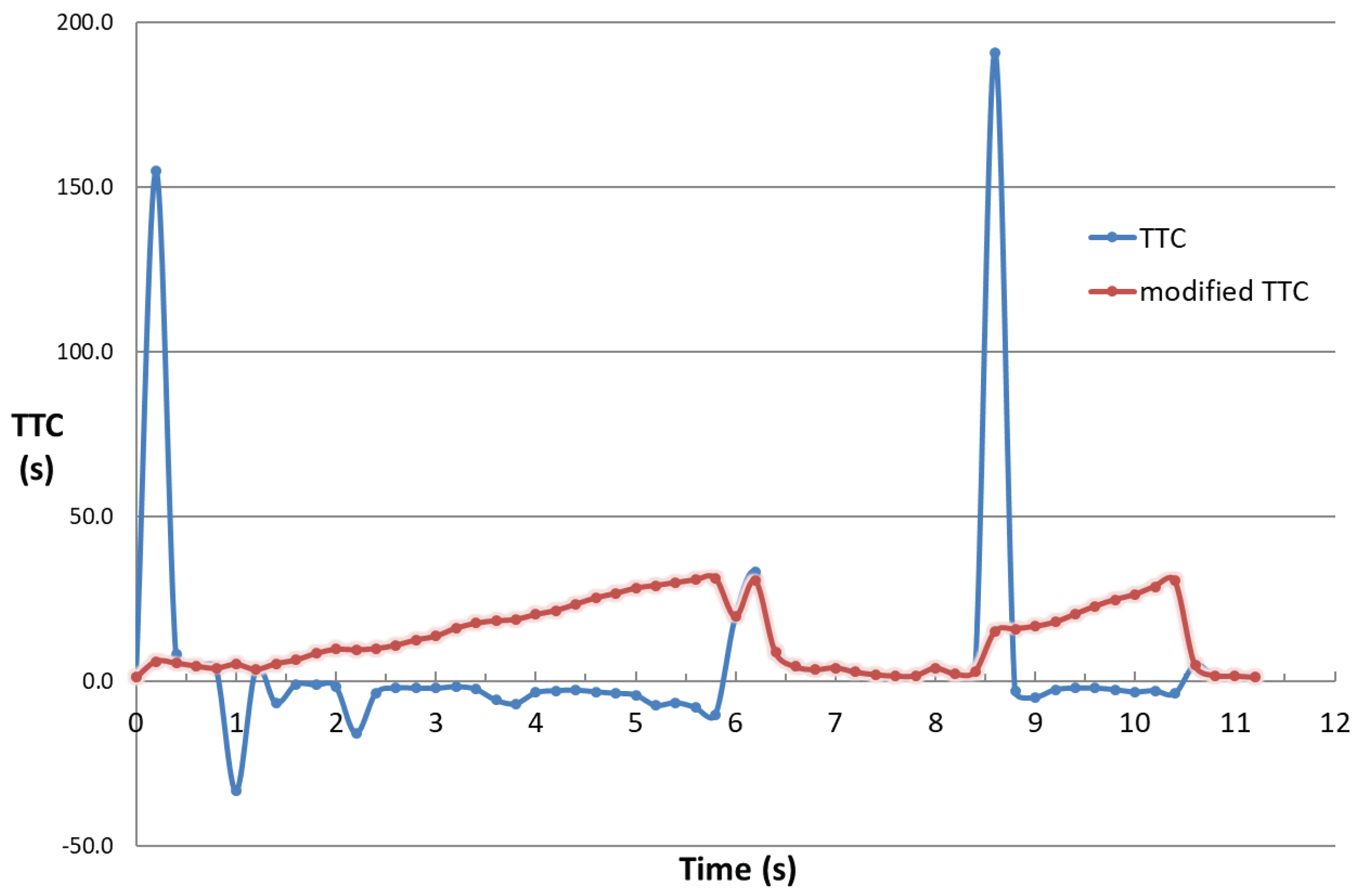
Figure 1 shows the TTC and modified TTC values calculated at 0.2 s intervals for a 12 s period. The TTC overestimated the collision risk during the 0–1 s and 8–9 s periods owing to a decrease in the relative speed and produced negative values when the preceding vehicle was faster than the following vehicle during the 1–6 s period. Conversely, the modified TTC generated positive values corresponding to the gap size between the two vehicles. These findings demonstrate that the modified TTC is more appropriate than the original TTC for use in continuous car-following situations. However, the modified TTC still has limitations, as it tends to distort the collision risk by assuming a constant

V_{F} (t) - V_{L} (t) = 1 k m / h

when the speed difference between the following and preceding vehicles is less than 1 km/h. To address this limitation, this study employed spectral analysis to estimate the collision risk in a more robust manner, independent of the traffic conditions.

4.2. Step 2. Calculation of PSD

Fourier [13] discovered that all periodic waves can be decomposed into a series of subordinate waves called harmonics, and each harmonic contains unique wave characteristics that can be analyzed through spectral analysis, which is a methodology for analyzing the energy distribution of a spectrum of frequencies. There are two main methods for spectral analysis: the Fourier series, which breaks down a periodic wave function into harmonics, and the Fourier transform, which converts a wave function from the time domain to the frequency domain. Spectral analysis is well suited for analyzing the relative speed waves in car-following situations because it can separate the waves into harmonics and analyze the energies of each component, including the collision risk.

A discrete Fourier transform was applied to transform a sequence of N complex numbers into another sequence of complex numbers (i.e., harmonics). If we define the aperiodic relative speed function observed over a particular time interval as

f (n)

, we can calculate the discrete Fourier transform

F [k]

f (n)

using Equation (3).

F [k] = \sum_{n = 0}^{N - 1} f (n) e^{- i 2 π k \frac{n}{N}}

(3)

The function

f (n)

represents the relative speed observed at the

n

(

n = 0,1, 2, \dots, N - 1)

-th time during a particular time interval. Therefore,

F [k]

represents the contribution rate of the

k^{t h}

(

k = 0,1, 2, \dots, N - 1)

harmonic of the relative-speed wave frequency. The energy distribution of the harmonics is represented by

{|F [k]|}^{2}

and is commonly used for comparison because

F [k]

contains complex numbers and is not suitable for direct comparison. Assuming that the cycle of

F [k]

is infinite,

P [k]

represents the PSD per unit frequency and can be calculated by dividing

{|F [k]|}^{2}

T

P [k] = \lim_{T \to \infty} [\frac{1}{T} {|F [k]|}^{2}] = \lim_{T \to \infty} [\frac{1}{T} F [k] F^{*} [k]]

(4)

where

F^{*} [k]

is the conjugate spectrum of

F [k]

and is calculated as follows

F^{*} [k] = \sum_{n = 0}^{N - 1} f (n) e^{- i 2 π k (- \frac{n}{N})} = \sum_{n = 0}^{N - 1} f (n) e^{i 2 π k \frac{n}{N}}

(5)

Equation (4) can be transformed into a discrete form as follows:

P [k] = \lim_{T \to \infty} [\frac{1}{T} F [k] F^{*} [k]] \approx \frac{F [k] F^{*} [k]}{N}

(6)

P [k]

calculated using Equation (6) represents the energy density of the individual harmonics in the frequency spectrum of the relative speed data. A high value of

P [k]

indicates that the corresponding harmonic significantly contributes to the overall change in the relative speed. Therefore,

P [k]

can be used to identify the most important frequency components for analyzing and understanding the dynamics of the car-following process.

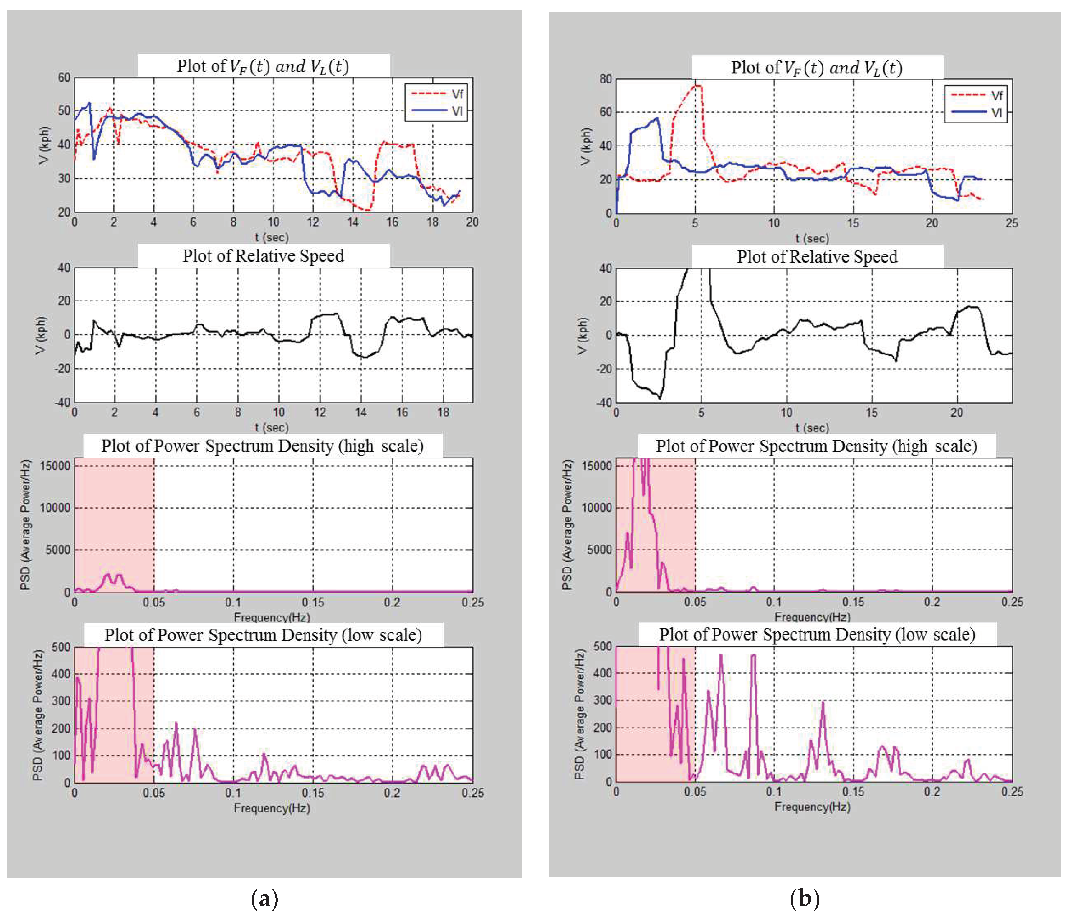
Figure 2 shows a comparison of the PSD of the relative speed data between safe and risky car-following situations using spectral analysis. The safe situation showed a low PSD value and a small range of frequency, indicating a similar scale of reaction to the stimulus and a small variation in the relative speed. In contrast, the risky situation shows a larger PSD value and a wider range of frequencies, indicating an amplified reaction to the stimulus and a larger variation in the relative speed caused by abrupt acceleration and deceleration. However, both situations show that the PSD is mostly concentrated at frequencies less than 0.05 Hz, indicating that long-period components or smooth variations in relative speed are prevalent.

For a more detailed analysis, the maximum PSD values on the y-axis were reduced from 15,000 to 500 Hz. This reduction in the PSD scale magnifies the medium-value PSD distributed over the frequency region above 0.05 Hz. In safe driving situations, the PSD of the relative speed is dominated by low-frequency components. As the frequency increases, PSD decreases significantly. The heavy concentration at the low-frequency speed components suggests that long-period components or smooth variations in relative speed are prevalent. Conversely, in risky driving situations, PSDs are excited over a wide range of frequencies and exhibit more high-frequency components than in safe driving situations. This implies that short-period components or large fluctuations in the relative speed caused by abrupt acceleration and deceleration are prevalent in risky car-following situations.

4.3. Step 3. Correlation Analysis between Modified TTC and PSD

We conducted a correlation analysis between the modified TTC and PSD,

P [k]

, to identify the frequency bands of the harmonics that exhibited a statistically significant correlation with the modified TTC. The modified TTC was calculated as the average over a time window of 15 s for the 170 datasets. If specific bands of harmonics were found to be correlated with the risky situation of the following vehicle, their

P [k]

values would also be correlated with the collision probability. Thus, it is possible to detect the risky driving situations of the following vehicle by performing a correlation analysis between the

P [k]

values and the modified TTC.

If there is a significant correlation between the specific frequency bands of the PSD and the modified TTC, the frequency bands can be utilized to calculate a surrogate measure for the collision risk of the following vehicle, which overcomes the limitations of the modified TTC mentioned earlier. The sum and ratios of the PSDs were calculated according to the frequency components and used in the correlation analysis. In this study, both the sum and ratio of the PSD were calculated in two ranges divided by the frequency value (0.05 Hz).

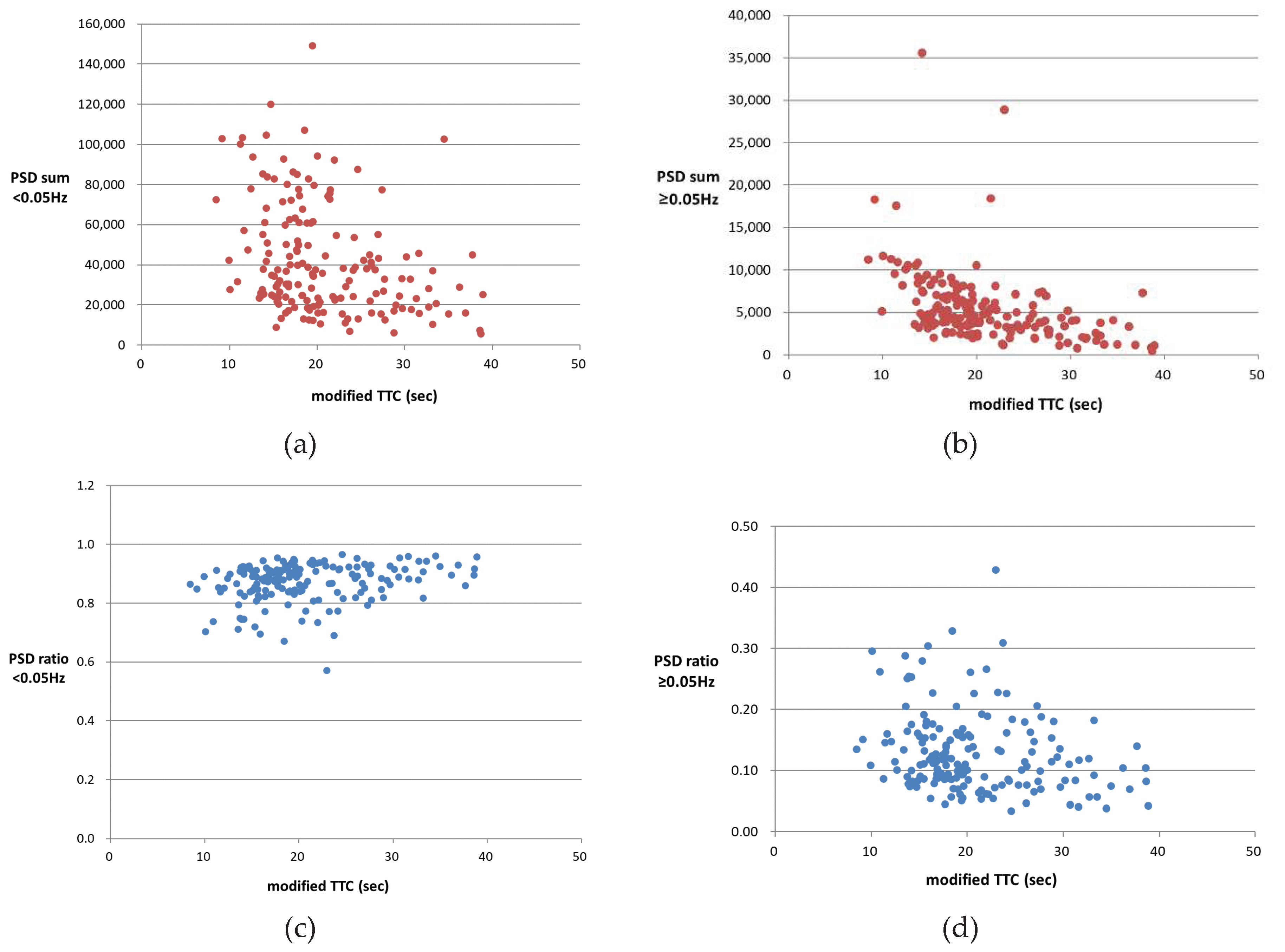
The high frequency of oscillations in the relative speed data, caused by frequent changes in the speeds of the following or preceding vehicles, results in a large sum of the PSDs. As the collision risk of both vehicles increased and the modified TTC decreased, the sum of the PSDs for both frequency ranges increased, as shown in Figure 3a,b. However, the PSD ratio shows a different correlation with the modified TTC depending on the frequency range. Specifically, Figure 3c,d show that the ratio of the PSD decreases at frequencies below 0.05 Hz whereas it increases at frequencies above 0.05 Hz, as the modified TTC decreases and collision risk increases. The correlation analysis between the PSD ratio and modified TTC presented in Table 1 shows that the frequency components ranging from 0 to 0.05 Hz have a positive correlation with the modified TTC. When the frequency range was segmented into 0.025 Hz (

\frac{1}{2}

of 0.05 Hz) and 0.0167 Hz (

\frac{1}{3}

of 0.05 Hz), the correlation coefficient in the 0–0.017 Hz range had the highest value (0.312), whereas negative correlation coefficients were observed in the other frequency bands. This positive correlation indicates that as the modified TTC increases, the energy density in the low-frequency components increases, suggesting a lower collision risk. The negative correlation coefficients in the other frequency bands indicate that as the energy density in these frequency components increases, the collision risk may also increase.

The p-value for all three frequency ranges was 0.000. The results of the correlation analysis suggest that the frequency components below 0.05 Hz, particularly in the range of 0–0.017 Hz, have a significant positive correlation with the modified TTC. The collision risk decreased when the ratio of the PSD at the frequency components in the range of 0–0.017 Hz increased. This indicates that the low-frequency components, which represent long-period changes in the relative speed, are more strongly related to the collision risk than the high-frequency components, which represent short-period fluctuations in the relative speed. These findings suggest that the low-frequency components of the PSD can be used as a surrogate measure of the collision risk in car-following situations.

Table 1. Correlation analysis over the segmented frequency ranges.

0.05 Hz interval			0.025 Hz interval			0.0167 Hz interval
Frequency (Hz)	Correlationcoefficient	p-Value	Frequency (Hz)	Correlationcoefficient	p-Value	Frequency (Hz)	Correlationcoefficient	p-Value
0–0.05	0.290	0.000	0–0.025	0.291	0.000	0–0.017	0.312	0.000
			0–0.025	0.291	0.000	0.017–0.033	−0.189	0.013
			0.025–0.050	−0.232	0.002	0.017–0.033	−0.189	0.013
			0.025–0.050	−0.232	0.002	0.033–0.050	−0.195	0.011
0.05–0.10	−0.264	0.001	0.050–0.075	−0.270	0.000	0.050–0.067	−0.239	0.002
			0.050–0.075	−0.270	0.000	0.067–0.083	−0.155	0.044
			0.075–0.100	−0.099	0.201	0.067–0.083	−0.155	0.044
			0.075–0.100	−0.099	0.201	0.083–0.100	−0.161	0.036
0.10–0.15	−0.213	0.005	0.100–0.125	−0.206	0.007	0.100–0.117	−0.208	0.006
			0.100–0.125	−0.206	0.007	0.117–0.133	−0.176	0.021
			0.125–0.150	−0.151	0.049	0.117–0.133	−0.176	0.021
			0.125–0.150	−0.151	0.049	0.133–0.150	−0.105	0.175
0.15–0.20	−0.175	0.023	0.150–0.175	−0.162	0.035	0.150–0.167	−0.159	0.038
			0.150–0.175	−0.162	0.035	0.167–0.183	−0.147	0.055
			0.175–0.200	−0.155	0.044	0.167–0.183	−0.147	0.055
			0.175–0.200	−0.155	0.044	0.183–0.200	−0.113	0.141
0.20–0.25	−0.221	0.004	0.200–0.225	−0.257	0.001	0.200–0.217	−0.192	0.012
			0.200–0.225	−0.257	0.001	0.217–0.233	−0.217	0.004
			0.225–0.250	−0.139	0.070	0.217–0.233	−0.217	0.004
			0.225–0.250	−0.139	0.070	0.233–0.250	−0.122	0.112

4.4. Step 4. Developmant of Driving Pattern Indices

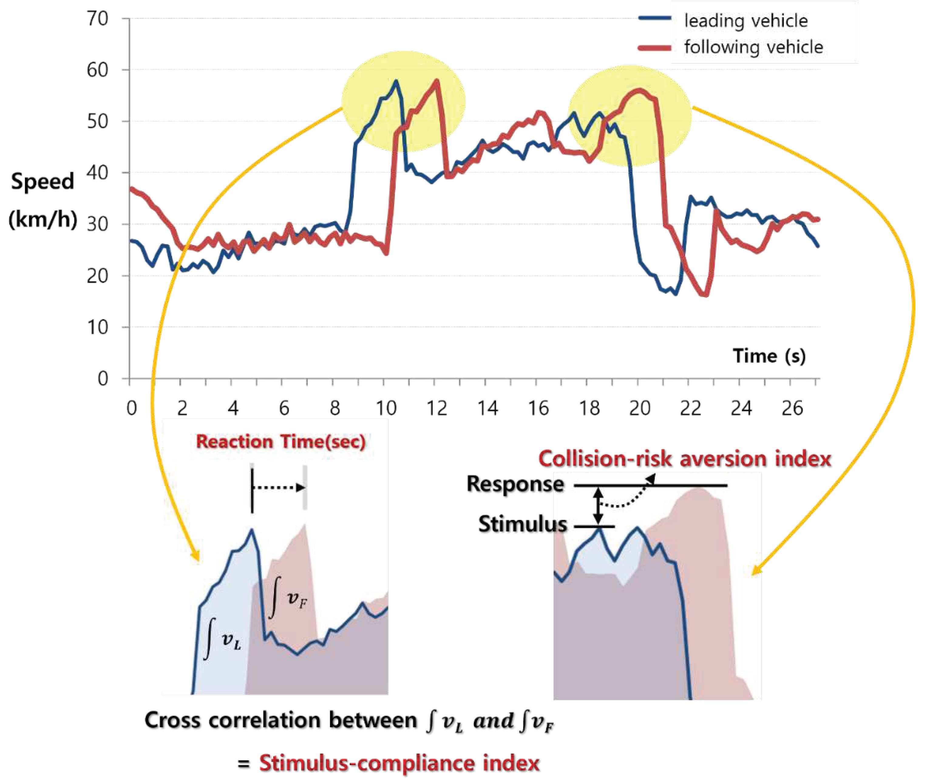
To assess the driving patterns of the following vehicles, we calculated three indices from the vehicle trajectory data in the car-following situation: reaction time, stimulus compliance index, and collision-risk aversion index (CRAI), as shown in Figure 4.

Reaction time and stimulus compliance index were determined from the cross-correlation of the speed data of the preceding and following vehicles. Let

(X_{t}, Y_{t})

represent a pair of the preceding and following vehicle speeds. The cross-correlation function and coefficient are given by Equations (7) and (8), respectively.

C_{X Y} (τ) = E [X_{t - τ} Y_{t}]

(7)

R_{X Y} (τ) = \frac{C_{X Y} (τ)}{σ X (t - τ) σ Y (t)}

(8)

where

τ

is the time delay between two speeds.

In a car-following situation, the following vehicle follows the preceding vehicle with an appropriate gap, speed, and acceleration. If the preceding vehicle accelerates or decelerates, the following vehicle adapts its speed with a certain time delay to reach the desired speed or safely proceed behind it. The reaction time is determined by the time delay that maximizes the cross-correlation coefficient and overlapping area of the two-speed data. The reaction time is an indicator of how quickly the following vehicle responds to changes in the speed of the preceding vehicle.

The cross-correlation coefficient was calculated using the time delay. If the cross-correlation coefficient is close to 1, then the following vehicle is more likely to conform to the stimulus of the preceding vehicle. If the cross-correlation coefficient is close to zero or has a negative value, the following vehicle is more likely to travel independent of the preceding vehicle. The stimulus compliance index is determined using the cross-correlation coefficient and reaction time

τ

. This is an indicator of how well the following vehicle conforms to the change in the speed of the preceding vehicle. A higher stimulus compliance index indicates better tracking of the speed of the preceding vehicle.

In Figure 5, the distribution of the stimulus compliance index is skewed toward 1, indicating that most of the following vehicles tend to conform to the speed changes of the preceding vehicle in car-following situations. The reaction time ranges from 0.80 to 4.20 s, with an average of 2.09 s, which is consistent with the assumption in most car-following models. The reaction time of 4.20 s was observed when the average distance headway was approximately 21.6 m, whereas the reaction time of 0.80 s was observed when the average distance headway was approximately 11.1 m.

The similarity in magnitude between the stimulus and response was indicated by the stimulus compliance index. The CRAI represents the extent to which the following vehicle tends to avoid collision risk. It was calculated by dividing the sum of the PSDs for the frequency components showing low collision risks by the total sum of the PSDs. In this study, the frequency range of 0–0.017 Hz was identified as the range with low collision risks. Therefore, the CRAI was calculated by dividing the sum of the PSDs in this frequency range by the total sum of the PSDs, as shown in Equation (9). A high CRAI value indicates that the following vehicle is more likely to maintain a safe distance from the preceding vehicle and avoid sudden acceleration and deceleration in response to the speed of the preceding vehicle, thereby reducing the risk of collision.

C o l l i s i o n - R i s k A v e r s i o n I n d e x (C R A I) = \frac{P S D o f h a r m o n i c s < 0.017 H z}{T o t a l P S D}

(9)

5. Results and Discussion

A correlation analysis was conducted to validate the CRAI of the following vehicle by examining the correlation between the PSD ratio and modified TTC using additional relative speed datasets. A total of 140 relative speed datasets collected from 27 May 2010 to 1 June 2010 at the same study site were used for this validation. The findings from the correlation analysis presented in Table 2 are consistent with those presented in Table 1, demonstrating a positive correlation coefficient in the frequency range below 0.017 Hz and negative correlation coefficients in the frequency ranges above 0.017 Hz. These results further support the validity of the CRAI calculation by dividing the sum of the PSDs below 0.017 Hz by the total sum of the PSDs.

To assess the applicability of the CRAI to real-world car-following situations, we compared the index with other traffic variables such as average travel speed, average relative speed, and space headway. Table 3 presents the results of the study. Our analysis found that the CRAI did not demonstrate a significant relationship with the average travel speed. However, a clear correlation was observed between the index and average relative speed (i.e., speed of the following vehicle − speed of the preceding vehicle). Specifically, the following vehicles with lower index values (i.e., more aggressive drivers) tended to exhibit higher average relative speeds and smaller space headways, which aligns with actual traffic accident scenarios. The proposed CRAI can be particularly useful for AVs in assessing the tendency of the following vehicles to engage in collision risk. By utilizing this index, AVs can plan safer driving strategies such as selecting appropriate car-following speeds and optimal gaps during lane-changing maneuvers.

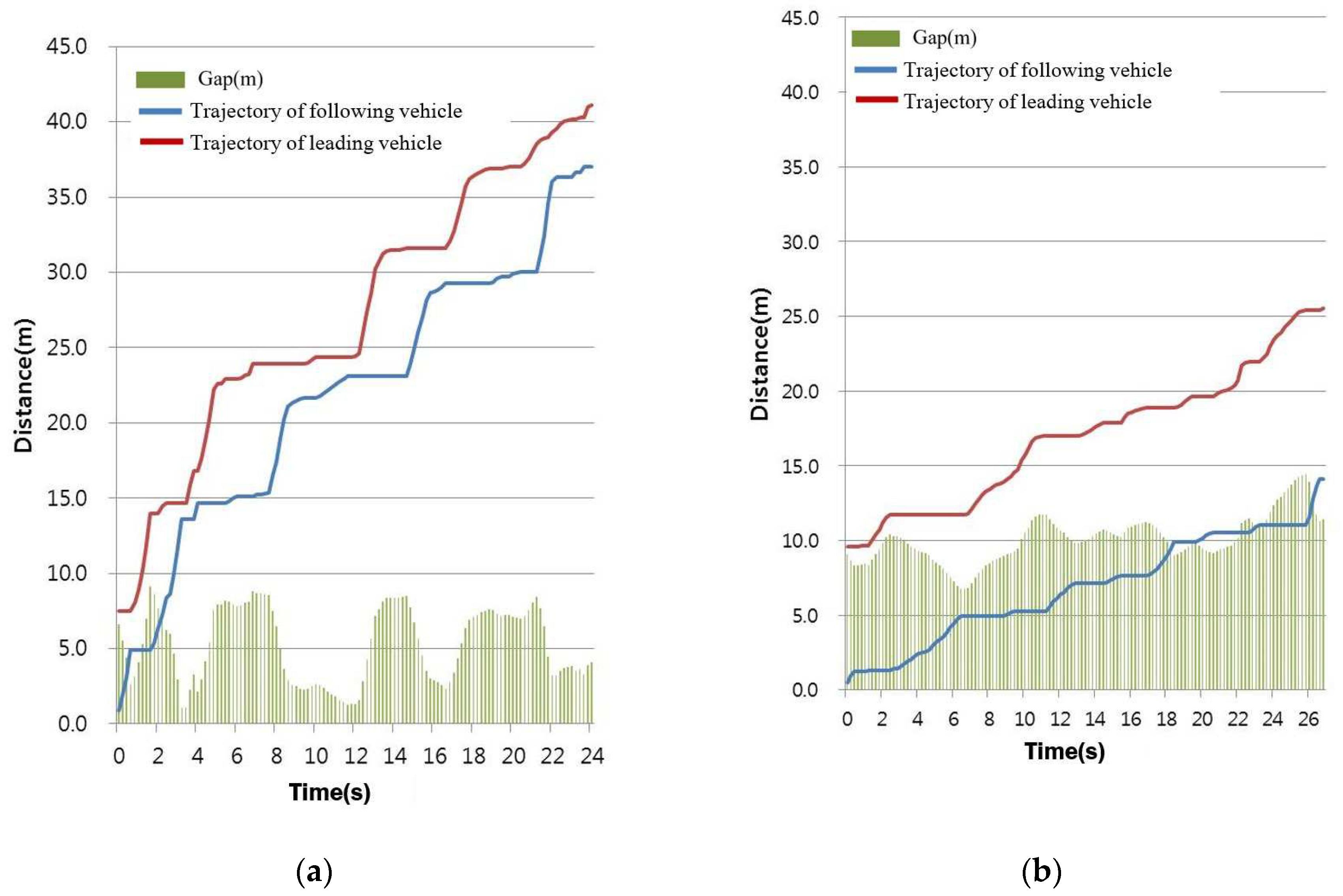
To demonstrate the efficacy of the CRAI developed in this study, two sets of preceding and following vehicle trajectory data are presented in Figure 7, representing high- and low-CRAI scenarios. The reaction time, stimulus compliance index, and other traffic variables were consistent between the two sets. However, for the trajectory with a low CRAI value (0.078), three risky situations occurred when the spatial headway was less than 1 m. During the observation interval, abrupt changes occurred in the space headway, and the following vehicle appeared to incur a collision risk. Conversely, in the trajectory with a high CRAI value (0.531), the space headway remained constant at approximately 10 m, that is, there were minimal changes in the space headway. These results highlight the CRAI as a valuable metric for identifying the driving pattern of the following vehicle.

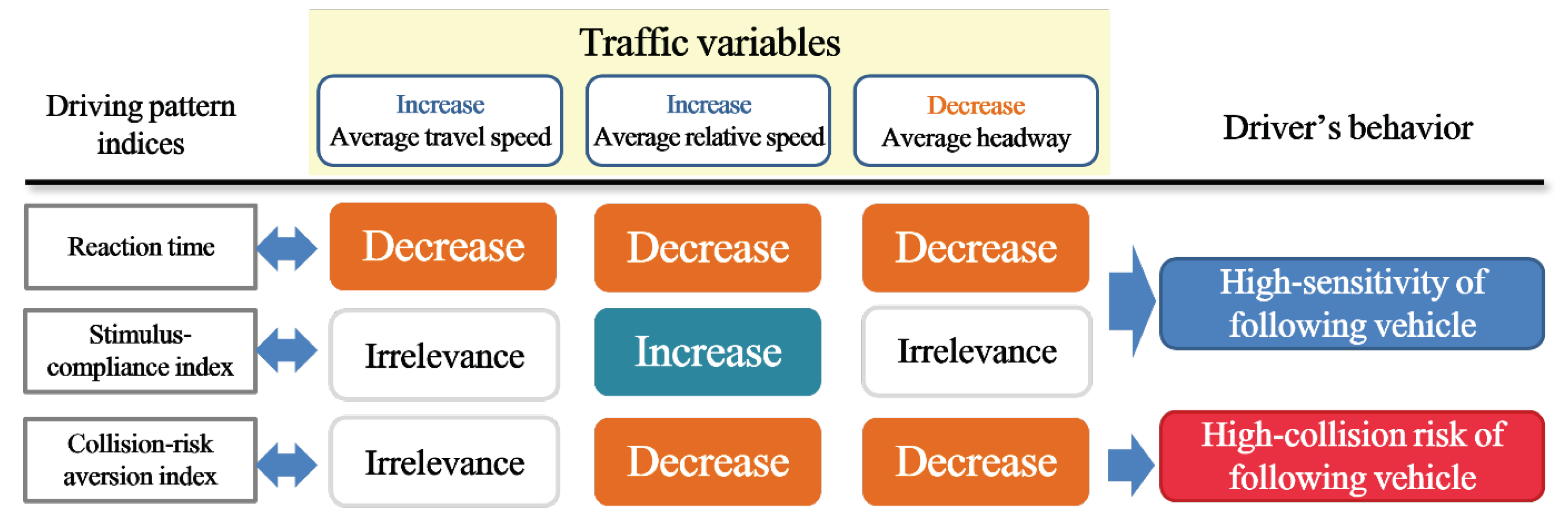
Based on the analysis of car-following situations, the relationship between driving-pattern indices and traffic variables was identified. This relationship is more apparent in risky car-following situations, as shown in Figure 8. In such situations, an increase in the average travel speed resulted in a decrease in the reaction time of the following vehicle, with no significant changes in the stimulus compliance index and CRAI. However, an increase in the average relative speed led to a decrease in both the reaction time of the following vehicle and the collision-aversion index, along with an increase in the stimulus compliance index. A decrease in the average headway corresponded to a decrease in both reaction time and CRAI, with no significant change in the stimulus compliance index. These findings suggest that in risky car-following situations, the following vehicles tend to exhibit higher sensitivity and aggressiveness, which is consistent with the results of existing research on traffic behaviors.

6. Conclusion

In this paper, we proposed a new methodology for identifying the driving patterns and collision risks of following vehicles based on relative speed data between the preceding and following vehicles collected during car-following situations. The proposed methodology can be used to develop effective measures for AVs to prevent rear-end collisions with following vehicles.

The contributions of this study are twofold: First, we propose a robust spectral-analysis-based technique for identifying the relationship between driving patterns and collision risks, which can be used in all traffic scenarios. This relationship can be further utilized to develop more effective methods for preventing rear-end collisions and improving traffic safety. Second, we propose a process to compute three indices—reaction time, stimulus compliance index, and CRAI to describe the driving pattern of the following vehicles. The behavior of risky drivers in car-following situations can be well described by these indices, which are consistent with the results of existing research. The collision risk aversion index is particularly useful for AVs in assessing the inclination of the following vehicles to engage in collision risks and plan safer driving strategies.

However, our proposed approach has limitations in field applications. The CRAI was developed for car-following situations; however, collision risks must be considered in various situations besides car-following, such as lane changing, merging, and weaving. Additionally, an extensive analysis of the threshold values of the index is suggested for future research.

Author Contributions

Data collection, Kim.; Methodology and Analysis, Chae., Writing—original draft, Chae.; Writing—review & editing, Kim. All authors have read and agreed to the published version of the manuscript.

Funding

This work was supported by a Korea Agency for Infrastructure Technology Advancement (KAIA) grant funded by the Ministry of Land, Infrastructure, and Transport (Grant RS-2022-00141102) and the authors are grateful to KAIA for economic supports.

Conflicts of Interest

The authors declare no conflict of interest.

References

National Highway Traffic Safety Administration (NHTSA). Traffic Safety Facts: 2019 Data; U.S. Department of Transportation: Washington, DC, 2020; Available online: https://crashstats.nhtsa.dot.gov/Api/Public/ViewPublication/813010.
Tak, S.; Kim, S.; Lee, D.; Yeo, H. A comparison analysis for surrogate safety measures with car-following perspectives for advanced driver assistance system. Journal of Advanced Transportation 2018, 2018, 8040815. [Google Scholar] [CrossRef]
Muzahid, A.J.M.; Kamarulzaman, S.F.; Rahman, M.A.; Murad, S.A.; Kamal, M.A.S.; Alenezi, A.H. Multiple vehicle cooperation and collision avoidance in automated vehicles: survey and an AI-enabled conceptual framework. Sci Rep 2023, 13, 603. [Google Scholar] [CrossRef] [PubMed]
Cabrera, A.; Gowal, S.; Martinoli, A. A new collision warning system for lead vehicles in rear-end collisions. IEEE Intelligent Vehicles Symposium: Madrid, Spain, 2012; pp. 674–679. [Google Scholar]
Kim, Y. Online traffic flow model applying the dynamic flow-density relation. Ph. D. Dissertation, Technical University of Munich, 2002. ISBN 0943-9455. [Google Scholar]
Treiber, M.; Kesting, A. Traffic flow dynamics: Data, Models. Springer, 2013; ISBN 978-3-642-32459-8. [Google Scholar]
Reuschel, A. Fahrzeugbewegungen in der Kolonne. Osterreichisches Ingenieur Archive 1950, 4, 193–215. [Google Scholar]
Pipes, L.A. An operational analysis of traffic dynamics. Journal of Applied Physics 1953, 24, 274–281. [Google Scholar] [CrossRef]
Gazis, D.C.; Herman, R.; Rothery, R.W. Nonlinear follow-the-leader models of traffic flow. Operations Research 1961, 9, 545–567. [Google Scholar] [CrossRef]
Gipps, P.G. A behavioural car-following model for computer simulation. Transportation Research part B 1981, 15, 105–111. [Google Scholar] [CrossRef]
Helly, W. Simulation of bottlenecks in single-lane traffic flow. In Proceedings of the Symposium on Theory of Traffic Flow, Research Laboratories, General Motors; 1959; pp. 207–238. [Google Scholar]
Hayward, J.C. Near-miss determination through use of a scale of danger. Highway Research Record 1972, 384, 24–34. [Google Scholar]
Fourier, J. The analytical theory of heat. Cambridge University Press, 1878; pp. 168–209. [Google Scholar]

Figure 1. Comparison of TTC and modified TTC.

Figure 2. Comparison of PSD: (a) Safe car-following situation, and (b) Risky car-following situation.

Figure 3. Corrrlation analysis between the modified TTC and PSD (a) Sum of PSDs for frequencies below 0.05 Hz, (b) Sum of PSDs for frequencies above 0.05 Hz), (c) Ratio of PSD for frequencies below 0.05 Hz, and (d) Ratio of PSD for frequencies above 0.05 Hz.

Figure 4. Driving pattern indices.

Figure 5. Histogram: (a) Stimulus-compliance index, and (b) Reaction time.

Figure 7. Vehicle trajectory: (a) Low CRAI (0.078), and (b) High CRAI (0.531).

Figure 8. Relationship between driving pattern indices and traffic variables in risky car-following situation.

Table 2. Validation of CRAI of following vehicle.

Frequency (Hz)	Initial Analysis Results		Verification Analysis Results
Frequency (Hz)	Correlationcoefficient	p-value	Correlationcoefficient	p-value
0–0.017	0.312	0.000	0.409	0.000
0.017–0.033	−0.189	0.013	−0.341	0.000
0.033–0.050	−0.195	0.011	−0.313	0.000
0.050–0.067	−0.239	0.002	−0.158	0.063
0.067–0.083	−0.155	0.044	−0.229	0.006
0.083–0.100	−0.161	0.036	−0.171	0.044
0.100–0.117	−0.208	0.006	−0.193	0.023
0.117–0.133	−0.176	0.021	−0.229	0.006
0.133–0.150	−0.105	0.175	−0.128	0.133
0.150–0.167	−0.159	0.038	−0.154	0.069
0.167–0.183	−0.147	0.055	−0.300	0.000
0.183–0.200	−0.113	0.141	−0.149	0.078
0.200–0.217	−0.192	0.012	−0.134	0.133
0.217–0.233	−0.217	0.004	−0.230	0.006
0.233–0.250	−0.122	0.112	−0.144	0.089

Table 3. Comparison of CRAI with traffic variables.

CRAI	Frequency	Average travel speed (km/h)	Average relative speed (km/h)	Space headway (m)
< 0.1	3	38.18	0.37	9.33
0.1–0.2	8	56.94	−0.14	12.72
0.2–0.3	16	41.66	−0.12	11.02
0.3–0.4	36	39.86	−0.32	13.09
0.4–0.5	44	39.99	−0.68	15.12
0.5–0.6	40	40.31	−0.82	16.24
0.6–0.7	17	35.66	−1.25	17.70
0.7–0.8	6	40.06	−0.79	36.23
0.8–1	0	-	-	-

Disclaimer/Publisher’s Note: The statements, opinions and data contained in all publications are solely those of the individual author(s) and contributor(s) and not of MDPI and/or the editor(s). MDPI and/or the editor(s) disclaim responsibility for any injury to people or property resulting from any ideas, methods, instructions or products referred to in the content.

© 2023 by the authors. Licensee MDPI, Basel, Switzerland. This article is an open access article distributed under the terms and conditions of the Creative Commons Attribution (CC BY) license (http://creativecommons.org/licenses/by/4.0/).

Copyright: This open access article is published under a Creative Commons CC BY 4.0 license, which permit the free download, distribution, and reuse, provided that the author and preprint are cited in any reuse.

MDPI Initiatives

Important Links

Choose an area of interest and we will send you notifications of new preprints at your preferred frequency.

Disclaimer

Investigation of Following Vehicle Driving Pattern using Spectral Analysis Techniques

Abstract

1. Introduction

2. Literature Review

3. Methodology

4. Driving-Pattern Assessment of Following Vehicle

4.1. Step 1. Modification of TTC

4.2. Step 2. Calculation of PSD

4.3. Step 3. Correlation Analysis between Modified TTC and PSD

4.4. Step 4. Developmant of Driving Pattern Indices

5. Results and Discussion

6. Conclusion

Author Contributions

Funding

Conflicts of Interest

References

MDPI Initiatives

Important Links

Subscribe